Iterative and Predictive Ray-Traced Collision Detection for Multi-GPU Architectures

HAL Id: dumas-00854986

https://dumas.ccsd.cnrs.fr/dumas-00854986

Submitted on 28 Aug 2013

HAL is a multi-disciplinary open access

archive for the deposit and dissemination of sci-entific research documents, whether they are pub-lished or not. The documents may come from teaching and research institutions in France or abroad, or from public or private research centers.

L’archive ouverte pluridisciplinaire HAL, est destinée au dépôt et à la diffusion de documents scientifiques de niveau recherche, publiés ou non, émanant des établissements d’enseignement et de recherche français ou étrangers, des laboratoires publics ou privés.

Iterative and Predictive Ray-Traced Collision Detection

for Multi-GPU Architectures

François Lehericey

To cite this version:

François Lehericey. Iterative and Predictive Ray-Traced Collision Detection for Multi-GPU Architec-tures. Graphics [cs.GR]. 2013. �dumas-00854986�

Master research Internship

Master thesis

Iterative and Predictive Ray-Traced Collision Detection for

Multi-GPU Architectures

Author:

Fran¸cois Lehericey

Supervisors: Val´erie Gouranton Bruno Arnaldi Hybrid Team

Abstract

Collision detection is a complex task that can be described simply: given a set of objects we want to know which ones collide. In the literature we can found numerous algorithms that depend on objects property, but we can’t find an overall solution that works on every objects.

The internship focuses on a recent algorithm that shot rays from the surface of objects in the direction of the inward normal, collision is detected if a ray touches the interior of another object. This method allows deep penetrations and gives instantly the information needed to separate the colliding objects.

To speedup this algorithm we present a novel ray-tracing based technique that exploits spacial and temporal coherency. Our approach uses any existing standard ray-tracing algorithm as a starting point and we propose an iterative algorithm that updates the previous time step results at a lower cost. In addition, we present a new collision prediction algorithm to evaluate whenever two objects have potentially colliding vertices. These vertices are inserted into our iterative algorithm to strengthen the collision detection.

The implementation of our iterative algorithm obtains a speedup up to 30 times compared to non-iterative ray-tracing algorithms. The use of two GPUs gives a speedup up to 1.77 times compared to one.

Keywords: Real-Time Physics-based Modeling, Collision Detection, Narrow Phase, Ray-tracing

Contents

Introduction 3

1 Bibliography 4

1.1 Collision detection . . . 5

1.1.1 Two step collision detection . . . 5

1.1.2 Physical response . . . 5

1.1.3 Performance in collision detection . . . 6

1.1.4 Broad Phase . . . 7

1.2 Narrow Phase . . . 7

1.2.1 Feature based . . . 7

1.2.2 Simplex based . . . 8

1.2.3 Bounding volume hierarchy . . . 9

1.2.4 Image based . . . 9

1.2.5 Synthesis of algorithms . . . 10

1.3 Studied Algorithm . . . 11

1.4 Ray tracing . . . 12

1.4.1 Ray intersection . . . 12

1.4.2 Ray tracing accelerating structures . . . 13

1.4.3 Work distribution impact on performances . . . 13

1.5 Conclusion . . . 13

2 Contributions 14 2.1 Iterative Ray-Traced Collision Detection . . . 14

2.1.1 Iterative Ray/Triangle-Mesh Intersection . . . 15

2.1.2 Ray/Triangle Intersection . . . 16

2.1.3 Predictive Ray/Triangle Intersection . . . 18

2.1.4 Iterative Ray-Tracing Criterion . . . 19

2.1.5 Concave and Missing Rays . . . 20

2.1.6 GPU and Multi-GPU . . . 20

2.2 Projected Constraints . . . 21

2.2.1 Constraint-based compatibility . . . 21

2.2.2 Constraints projection . . . 22

2.3 Performance Comparison . . . 22

2.3.1 Experimental Setup . . . 23

2.3.2 Standard Ray-Tracing algorithms used . . . 24

2.3.3 Overall Simulation Performances . . . 25

2.3.4 Iterative Ray-Tracing Performances . . . 26

2.3.5 Multi-GPU Performances . . . 27

2.3.7 Projected Constraints Performances . . . 28

Introduction

In virtual reality (VR) and others applications of 3D environments, collision detection (CD) is an essential task. Given a set of objects, we want to know which ones collide. Although this formulation is simple, collision detection is currently one of the main bottlenecks of VR application because of the real-time constraint imposed by the direct interaction of the user and the natural complexity (O(n2_{)) of the naive algorithms.}

Figure 1: Real-time simulations with 1000 and 2600 objects from [Avr11]

One of the most challenging problem in collision detection is scalability in term of number of objects under the real-time constraint. We want to simulate thousands of objects (as can be seen in figure 1) or even hundreds of thousands of objects in real-time. Obviously simulate 300 000 objects with collision at 100 Hz is very complex, thus we are looking for algorithms with the lower complexity possible.

Chapter 1 presents the bibliography made before the internship. The purpose was study the state of the art to find possible contributions. Chapter 2 lists the contributions that have been made during the internship and the experimental results that prove their efficiency.

Chapter 1

Bibliography

Collision detection is a complex task that can be described simply: given a set of objects we want to know which ones collide. In the literature we can found numerous algorithms that depend on objects property, but we can’t find an overall solution that works on every objects. We focus on a recent algorithm that shot rays from the surface of objects in the direction of the inward normal, collision is detected if a ray touches the interior of another object. This method allows deep penetrations and gives instantly the information needed to separate the colliding objects.

There is a lot of parameters when we deal with collision detection [Avr11]. First we have to deal with a large variety of object. Objects can be concave or convex, with or without holes. Objects can be solid, deformable, liquid and have topology changes (they can split or merge). Objects can be represented with polyhedrons (generally with triangle faces), CSG (Constructive Solid Geometry) or parametric functions. We also have to deal with several parameters on the overall simulation. We can work on 2-Body (one object against a fixed environment) or N-Body (N objects moving independently). Simulation can be continual or discrete. All these parameters can change the method used in collision detection, this have created a lot of quite different solutions that we will expose.

The aim of the internship is to make a contribution on one of these methods. We will look for an algorithm that can work with:

• Concave objects

• Solid and deformable objects without topology changes

• objects represented with polyhedrons or basic volumes (sphere, rectangular box, ...) Concerning the simulation we would like:

• N-Body simulation • discrete simulation

Section 1.1 exposes general trends in collision detection. Sections 1.2 lists the existing algorithms in the narrow phase of collision detection. Section 1.3 presents in detail the algorithm on which the internship will focus. Section 1.4 gives a background knowledge that will be necessary to implement the selected algorithm. Section 1.5 concludes the bibliography.

1.1

Collision detection

We first in section 1.1.1 presents how collision detection is decomposed nowadays in two phases. Section 1.1.2 is about what appends after a collision is detected: physical response. Section 1.1.3 introduces new trends regarding performance. Section 1.1.4 briefly details the first phase of collision detection.

1.1.1 Two step collision detection

When working with n objects, the naive approach trends to have a O(n2_{) complexity by testing}

all pairs of objects. To break down the complexity, since Hubbard [Hub93], collision detection is decomposed in two phases, the broad-phase and the narrow-phase. The broad-phase plays the role of a filter by performing a quick collision test, the aim is to quickly remove non-colliding objects. The narrow-phase works with the pairs that passed the broad-phase. These pairs are in potential collision and the goal of the narrow-phase is to perform exact collision test and gives contact or interpenetration information so physical response can be computed.

Figure 1.1 exposes the collision detection pipeline. First the pipeline is fed with geometric data. The broad-phase handles these objects and output pairs of potentially colliding objects. The narrow-phase processes these pairs and output the ones that really collide. At the end the physical response module computes the new position of objects depending of the collision and the contact information.

GEOMETRIC

DATA

BROAD

PHASE

NARROW

PHASE

RESPONSE

PHYSICAL

objects

Pairs of

objects

_{Contact information}

Colliding pairs

+

Figure 1.1: Collision detection pipeline

1.1.2 Physical response

There are several algorithms concerning the physical response[MW88]: penalty-forces, impulse-based constraint-impulse-based and position-impulse-based. Penalty-forces is the most simple and works on acceleration (second derivative of the position), when a collision happens we apply a force proportional to the interpenetration to separate the objects. This method is equivalent to add springs on collision, this may cause oscillation in the position of objects. Impulse-based method works on the velocity (first derivative of the position), when a collision happens we apply impulsion on the velocity to separate the objects. This method solves the problem of oscillating objects presents in Penalty-forces response. These two first methods have difficulties when several objects are present with several colliding contacts, the third method have been

introduced to solve these cases. Constraint-based method computes the exact forces needed at each step to avoid interpenetration, but instead of working on each colliding pair independently, work on a global solution with a solver. This method works with several contacts points but requires more computation. Position-based methods works directly on the positions [BMOT12], these methods are fast and stable but are not physically correct (the result is visually plausible).

1.1.3 Performance in collision detection

New ways of improvements are always been used to accelerate collision detection. One way to improve performance is to use parallelism. Parallelism can be used to get better performances on multi-cores architectures [Avr11] but also can be used in grid architectures.

Collision detection is decomposed in two phases, and a synchronization is present between the two phases to assure consistency. With parallelism this synchronization will become a problem because it will make core wait with no work. We can refine the two phase as a pipeline [AGA+_{10] where pairs of objects transit. This allows to break the synchronization between the}

two phases to achieve better performances.

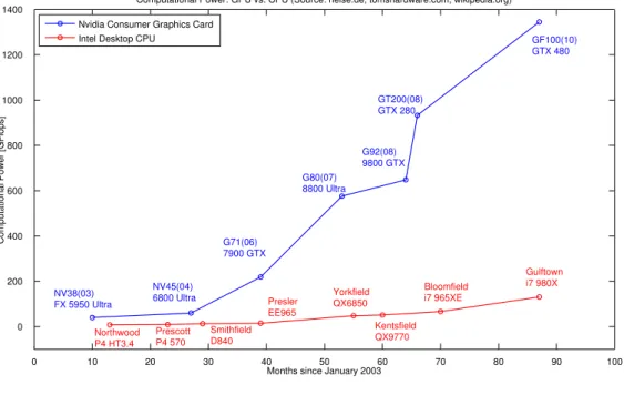
More recently General Purpose GPU (GPGPU) allowed to perform heavy computation on GPU with OpenCL or CUDA, the goal is to use the rising power of GPU. Figure 1.2 shows that since 2005 the computational power of GPU is higher and grows faster than CPU, this means an algorithm will theoretically run faster on GPU. These new tools have been used to improve performances in collision detection [Kno03] [WFP12].

Months since January 2003

C om p u ta ti o na l P o we r [G F lo p s]

Computational Power: GPU vs. CPU (Source: heise.de, tomshardware.com, wikipedia.org)

NV38(03) FX 5950 Ultra NV45(04) 6800 Ultra G71(06) 7900 GTX G80(07) 8800 Ultra G92(08) 9800 GTX GT200(08) GTX 280 GF100(10) GTX 480 Northwood P4 HT3.4 Prescott P4 570 Smithfield D840 Presler EE965 Yorkfield QX6850 Kentsfield QX9770 Bloomfield i7 965XE Gulftown i7 980X 0 10 20 30 40 50 60 70 80 90 100 0 200 400 600 800 1000 1200 1400

Nvidia Consumer Graphics Card Intel Desktop CPU

Figure 1.2: Evolution of CPU and GPU (gpu4vision.icg.tugraz.at)

GPUs are composed of thousands of core, to exploit their computational power we have to give them highly parallelizable tasks. Generally, GPGPU frameworks require to get the work

in the form of iterations (in several dimensions). An important property of GPUs is they do not have caches like CPUs, random memory access have a higher cost on GPUs than on CPU. With these properties, algorithm that underperform on CPUs can outperform on GPUs. It is also possible taht algorithm that outperform on CPUs underperform on GPUs.

1.1.4 Broad Phase

This section lists the principals broad-phase algorithms. The broad phase takes as input a set of objects and output a set of potentially colliding pairs. This phase is simpler than the narrow phase and is less critical nowadays for performance. Thus we won’t detail each algorithm. The classification of these algorithms come from Quentin Avril’s thesis [Avr11].

Brute force The brute force is a test of every pair of object’s bounding volume. This is the most simple broad-phase algorithm, but the complexity is O(n2_{) because if we have n}

objects n2

−n

2 pairs are tested.

Spacial partitioning The idea is, if two objects are distant they will not collide. In these algorithms objects are stored in data structure that partition space (grid, octree, kd-tree, ...) and then run through these structures to locate potentially colliding objects

Cinematic The idea is, if two non colliding objects move away then they will not collide. Topology We work on projection with one theorem, if two objects are colliding then they are

colliding on every projection. The idea is to check several projections and only keep the pairs of objects that collide in every projection. The most famous topology algorithm is Sweep and Prune, which works with projections on x, y and z-axis.

1.2

Narrow Phase

The narrow phase takes as input the set of potentially colliding pairs from the broad phase and outputs a set of colliding object and information about the contacts between objects. This section lists the principal narrow-phase algorithms. Section 1.2.1 presents feature based algorithms. Section 1.2.2 presents simplex based algorithms. Section 1.2.3 presents bounding volume hierarchy. Section 1.2.4 presents image based algorithms. At the end, section 1.2.5 compare the algorithms and decide on which one we focus. All the algorithm are presented for a 2-body collision as the narrow phase input pairs of object, even through some of the algorithms could be used with more objects. The classification of these algorithms come form surveys [TKH+_{05] [KHI}+_{07] and [Avr11].}

1.2.1 Feature based

Feature based algorithms directly work on geometric primitives of objects. The most famous algorithms are polygonal intersection of Moore and Wilhelms, Lin-Canny, V-Clip and SWIFT. The main idea of these algorithms is to find the two closest points between two objects, and test if each point is inside or outside other object.

Moore and Wilhelms [MW88] test if a representative point of one object is inside the other one. For the objects A and B, each vertices of A is tested on the object B and then each vertices of B is tested on the object A. The algorithm stops and a collision is detected if one point is inside the other object, otherwise there is no collision.

Lin-Canny [LC91] proposed to track the closest feature instead of the closest point, a feature can be a vertex, an edge or a face. V-Clip (Vorono¨ı-Clip) is based on Lin-Canny space around each object is divided into vorono¨ı regions, these cells indicate for every points outside the object what is the closest feature (vertex, edge or face). The aim is to find the two closest feature F(A) and F(B) between two objects A and B, and then P(A) and P(B) the two closest points on F(A) and F(B). The two closest feature satisfy the property: P(A) is in the vorono¨ı region of F(B) and P(B) is in the vorono¨ı of F(A). Figure 1.3 gives an example of two closest points and their matching vorono¨ı regions. Here F(A) is the edge supporting P(A) and F(B) is the vertex P(B).

A

B

of F(A) voronoï regionof F(B)

Figure 1.3: Lin-Canny algorithm: P(A) and P(B) are the two closest points

1.2.2 Simplex based

Simplex based algorithms work on the convex hull of objects. This mean these algorithms are incorrect for concave objects, but can be used as a filter before launching more complex algo-rithms. The most famous simplex based algorithm is GJK (Gilbert-Johnson-Keerthi) [GJK88]. Instead of directly work on the two object, the algorithm works on the Minkowski difference.

For two convex object A and B composed of points x ∈ A and y ∈ B we are looking for a colliding pair (x, y) where x = y. The Minkowski difference is defined as AΘB = {x − y : x ∈ A, y ∈ B}. We can use the Minkowski difference to simplify the search of x = y by testing if −

→

0 ∈ AΘB, this simplifies the search because instead of having two unknown variable we only have one. An example of a Minkowski difference is illustrated in figure 1.4.

We have now to test if −→0 ∈ AΘB and we know that AΘB is convex due to Minkowski difference property, this mean we can apply basic algorithms to quickly test if −→0 is inside or outside the difference.

Several improvements have been proposed for the GJK algorithm, the most important ones are: Enhancing GJK [Cam97] uses hill climbing to speed up the process. ISA-GJK [VdB99] uses data caching and image coherence between successive frame of animations.

B A

O

AΘB

Figure 1.4: Exemple of a Minkowski difference on two polygons. AΘB is the difference between A and B.

1.2.3 Bounding volume hierarchy

A bounding volume hierarchies (BVH) is a tree of primitives representing bounding volumes (BV). The object is partitioned with primitive organized in a tree, each node is a bounding volume of all his children. Leafs can be a single primitive of the object, or several primitives. The root of the tree is a bounding volume of the whole object. In BVH the choice of BV is important because it have an impact on performance. The principals BV are: sphere, Oriented Bounding Box, Axis Aligned Bounding Box, Discrete Oriented Polytope, spherical shell and convex hull. Figure 1.5 illustrates these principals bounding volumes. Collision detection against two objects (or self collision detection) are calculated by traversing the BVH top-down.

Sphere

OBB

AABB

DOP

Spherical

shell

Convex

hull

Figure 1.5: Examples of bounding volumes

A problem is the construction of BVH for a given object. Generally BVH are calculated only once and before computations, thus computation time is not the main problem. For rigid objects the aim is to minimize the time of collision detection queries. For deformable object we also want to minimize the time needed to update the BVH after deformation. Updating a BVH is possible if there is no topology change.

BVH are known to be among the most efficient structure for collision detection. Application of BVH have shown that binary tree have worst performances than 4-ary 8-ary trees. For deformable object AABBs are preferred because their update are cheap.

1.2.4 Image based

Image-based approaches use image rendering techniques to detect collision, they can often be executed on GPU since they are designed to execute rendering algorithms. We can decompose image-based approaches in two categories, depth-peeling and ray-casting.

Depth-peeling uses Layered Depth Image (LDI) to linearize the process as Z-buffer linearize the rendering time. LDI is a pixel matrix, unlike the Z-buffer that only keep the distance of the closest point for each pixel, LDI uses layers to keep every layer. Allard and al. [AFC+_{10] use}

LDI to detect collision and compute the physical response. The main drawback of depth-peeling is the discretization introduced by the LDI, this may cause errors (small objects may not be detected). An example of a LDI is given in figure 1.6.

Figure 1.6: 2D slice of an LDI between two objects, the intersection volume is in purple (from [AFC+_10]).

Ray-casting techniques render LDI with ray-casting. Wang and al. [WFP12] launch rays form an irregular grid to compute LDI. The density of ray is higher around small objects to not miss them (this may happen with depth-peeling). Cinder algorithm [Kno03] cast rays from the edges of an object and counts how many object face the ray passes through. If the result is odd then there is collision otherwise not. These rays are cast toward a regular grid.

Hermann and al. [HFR+_{08] propose a new approach where rays are cast from the vertices}

of an object in the opposite direction of the normal. If one of these rays intersect the other object form the inside, there is collision. The advantage of this method is it doesn’t need heavy computation to get contact information for the physical response, because the length of the intersecting rays are sufficient.

1.2.5 Synthesis of algorithms

We have to select one algorithm on which we will focus and propose a contribution, the algorithm must have the properties we listed in the introduction:

• Work with concave objects

• Manage solid and deformable objects without topology changes

• Work with objects represented with polyhedrons or basic volumes (sphere or rectangular box)

For each category of algorithm, we check the three properties:

Feature based These algorithms can work with concave objects but usually need pretreatment that can be heavy for deformable object.

Simplex Based Simplex Based algorithms can’t work with concave object, consequently we will not work with them.

Bounding Volume Hierarchy These algorithms work with concave objects and they can be extended to deformable objects but with extra computations.

Image based Image based techniques work on concave objects and deformable objects with no extra-computations. They usually introduce small errors due to the discretization. We can notice that Hermann algorithm [HFR+_{08] does not suffer of errors due to discretization.}

We decided to work on Hermann algorithm, all the requirements are met and the algorithm had never been tested on GPU. We will consequently focus on the implementation of Hermann algorithm on GPU.

1.3

Studied Algorithm

This section presents in details Hermann [HFR+_{08] collision detection algorithm.}

Hermann’s algorithm detect collision with rays launched from the vertices of an object in the opposite direction of the normal. Figure 1.7 shows an example on two objects, the plain arrows are three rays that spot collision, the dotted arrow is a rejected ray because it hits the other object from outside.

Figure 1.7: Illustration of [HFR+_{08] in 2D}

One advantage of this algorithm is the information given for physical response. For a lot of other narrow phase algorithms, when a collision is spotted additional computation is needed to compute the physical response. Hermann’s algorithm gives for each penetrating vertex a direction and a distance to separate the two objects (as can be seen in figure 1.7), these distances can be use to easily compute the physical response which is a great advantage compared to the others algorithms. According to the authors one other advantage is that the algorithm does not depend on precomputed data so it’s can be used on deformable objects, this is not entirely true because accelerative structure for ray-tracing needs to be updated.

The algorithm works on polyhedrons but it can be generalized. Ray are launched from ver-tices, these vertices can be view as a sampling of the surface, this mean that we can launch rays from any surface by using sampling. After launching the rays we have to detect the first inter-section with the other object, this can be achieved with any kind of objects. This generalization shows that we can use Hermann algorithm on any objects, this includes polyhedrons, CSG and

parametric functions. This generalization also means we can compute collision detection for pairs of objects of different nature (for example polyhedron vs CSG).

This algorithm have been implemented on CPU by Hermann but not tested on GPU, Kim and al. [KKL+_{10] have successfully implemented it without any mention of GPU programming.}

It would be interesting to implement this algorithm on GPU and compare its performances with other algorithms.

1.4

Ray tracing

This section presents essentials ray tracing technique that will be used to implements Hermann algorithm. First section 1.4.1 present rays intersection algorithms with triangle and basic ob-jects. Secondly section 1.4.2 introduce accelerating structures. In section 1.4.3 we present the effect of work distribution on performances.

1.4.1 Ray intersection

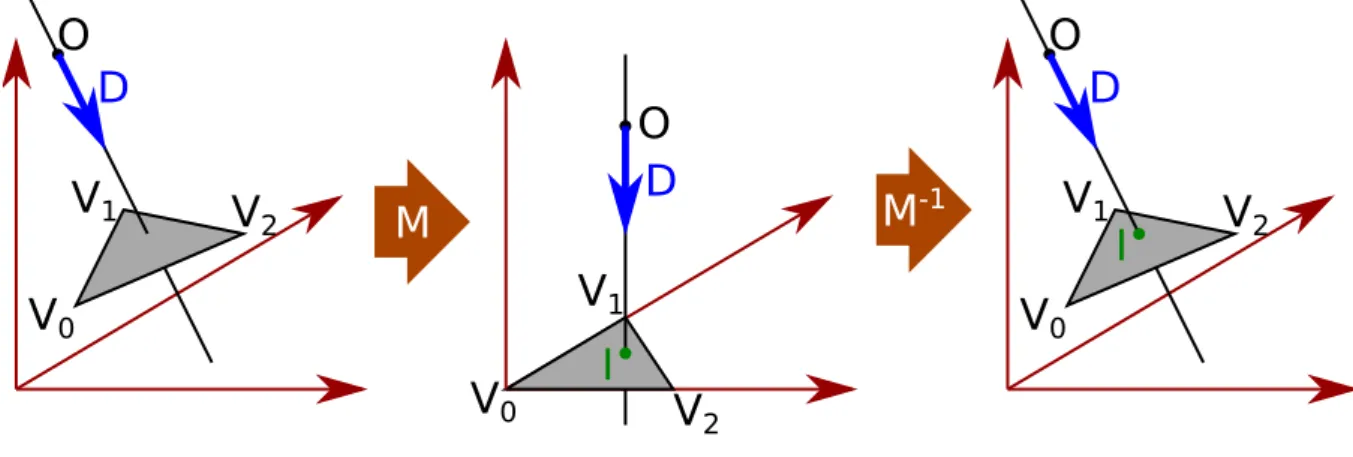
For polyhedrons we need to quickly perform ray-triangle intersection since this operation will be performed repeatedly. M¨oller and Trumbore [MT97] propose a simple algorithm with no precomputation. The algorithm does not give the coordinate of the intersection point in the space, instead it computes the intersection point in both triangle-space and ray-space coordinate. Figure 1.8 show the mains steps of the algorithm. We start with a triangle defined by three vertices (V0, V1, V2) and a ray defined by an origin and a direction O + tD. The main idea is to

find a transformation M that turn the triangle into a unitary triangle in the plane (y, z) and align the ray with the x-axis. In this situation the intersection point I can easily be localized and we can use M−1 _{to get the coordinates of I in the original space.}

V

V

V

O

D

V

V

V

O

D

V

V

V

O

D

I

I

M

M

Figure 1.8: M¨oller ray-triangle intersection

For basic objects, we can use algorithms from ACM SIGGRAPH HyperGraph1_{which gathers}

essential algorithms in the fields of Graphics, including ray tracing.

1

1.4.2 Ray tracing accelerating structures

Several accelerating structures have been proposed to improve the performance of ray tracing rendering. Thrane and al. [TS+_{05] made a comparison of the main accelerative structures and}

showed that BVH have the best performances.

Gunther and al. [GPSS07] present a ray tracing algorithm for GPU, they use a BVH with AABBs (Axis Aligned Bounding Box). The article presents the BVH construction as well as the ray traversal algorithm.

1.4.3 Work distribution impact on performances

GPUs are SIMT machines (Single Instruction Multiple Threads), the major restriction is threads cannot work independently. Threads work in group and have to wait each other before finishing or switching context. These restriction make load balancing a major cause of inefficiency went developing on GPUs.

In the case of ray tracing this problem is recurrent because ray casting is not a regular algorithm and the computation time of each ray cast can vary. Aila and al. [AL09] have tested different load balancing algorithms for ray tracing. They propose a load balancing algorithm that improve ray tracing performance. The idea is, instead of launching one ray per thread, to use a global pool in which the treads fetch the work. This is possible to implements with an atomic counter. This replace the waiting time with a fetch and thus limit idle time.

1.5

Conclusion

Collision detection is one of the main bottleneck in virtual reality. Collision detection is nowa-days organized as a two phase pipeline in the broad-phase and the narrow-phase. In this pipeline the most time consuming part is the narrow-phase on which we focus. We looked of an algo-rithm that works with concave objects, solid and deformable objects and polyhedrons and basics volumes.

Hermann algorithm allow fast collision detection, it rely on image based techniques without suffering from errors caused by discretization because the rays are not cast form a grid but from the objects vertices. This algorithm does not need extra computations to get the contacts information. This algorithm can be easily parallelized which make it a perfect candidate to be ported on GPU. In the internship we will test the algorithm on GPU and then compare it’s performances with other algorithms.

In recent physics engine the narrow phase does not work with one algorithm but with several. Depending on the nature of the two objects the best algorithm is selected. This choice is made with a table where rows and columns are the type of the object and each box it the best algorithm. It will important to compare the performances of Hermann algorithm in every case it can be applied (convex/convex, concave/convex, convex/sphere, ...) because there may be improvements for specific cases.

Chapter 2

Contributions

The internship have focused on Hermann and al. [HFR+_{08] algorithm, this chapter presents}

the contributions we made on the algorithm performance in term of speed and detection. Section 2.1 presents a novel iterative ray-tracing technique that exploits spacial and temporal coherency. Our approach uses any existing standard ray-tracing algorithm as a starting point and we propose an iterative algorithm that updates the previous time step results at a lower cost. Our iterative ray-tracing algorithm is applied in Hermann and al. technique to speedup the collision detection. In addition, we present a new collision prediction algorithm to evaluate whenever two objects have potentially colliding vertices. These vertices are inserted into our iterative algorithm to strengthen the collision detection. Section 2.2 explains why the directions of the rays are not adapted for constraint-based physical response and how to adjust the rays in that case. Section 2.3 gives the experimental performances of our contributions.

This work has been submitted to ACM VRST (Virtual Reality Software and Technology) as a full paper entitled ”New Iterative and Predictive Ray-Traced Collision Detection Algorithm for Multi-GPU Architectures” by Fran¸cois Lehericey, Val´erie Gouranton and Bruno Arnaldi.

2.1

Iterative Ray-Traced Collision Detection

Collision detection has to be performed at each simulation step. With ray-traced techniques, rays are cast from scratch at each simulation step for each pair of object. Instead we propose to use an iterative ray-tracing that takes advantage of the temporal coherency between the objects in each pairs.

In this section we present our iterative ray-tracing technique that can be used to speed up collision detection that valid for both convex and concave cases. Section 2.1.1 presents the overall principle of the technique for triangle meshes. Section 2.1.2 focuses on the ray/triangle intersection. Section 2.1.3 presents our predictive collision detection algorithm that avoids missing new penetrating vertices in the iterative algorithm. Section 2.1.4 explains the criterion to jump between iterative and non-iterative technique. Section 2.1.5 justifies why our iterative ray-tracing technique that theoretically works only with convex object can be used with concave

objects and why we can tolerate missed rays. Section 2.1.6 explains how we can use GPU (and several GPUs) to increase the performances.

2.1.1 Iterative Ray/Triangle-Mesh Intersection

As mentioned before, we follow Hermann and al. [HFR+_{08] algorithm. For each pair of object}

we cast a ray form each vertex in the opposite direction of the normal, if the ray hits the other object before leaving the source object collision is detected. An important optimization is to only cast ray form vertices that are inside the intersection of the bounding volumes of the two objects.

The main idea of iterative ray/triangle-mesh intersection is to use a standard algorithm to get the first intersection and to use an iterative algorithm on the next steps to update the previous result. The standard algorithm can be any algorithm (including those presented in section 1.4.2). The only important modification is to record for each ray the reference of the impacted triangle.

Our algorithm relies on an adjacency list between each triangle through the edges. For each ray, the iterative algorithm starts from the previous impacted triangle and tries to follow the path of the ray on the triangle mesh (cf Algorithm 1). We cast the ray into the previously impacted triangle, we then have two cases:

• The ray hits the triangle. The algorithm stops and the intersection is found.

• The ray misses triangle. We select the edge that closest to the ray (explained in sec-tion 2.1.2), get the corresponding triangle through the adjacency list and reiterate the algorithm.

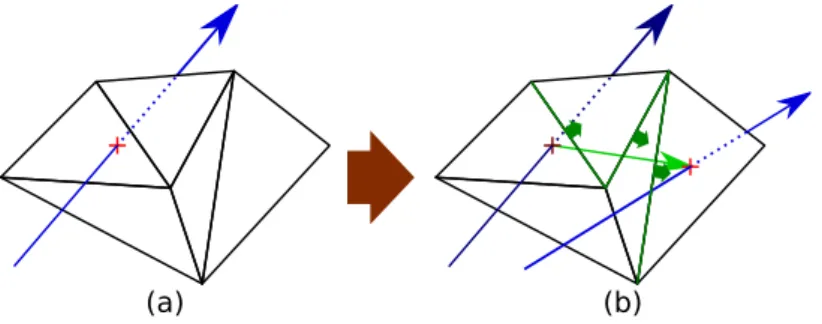
When the ray does not hit the previous triangle, the algorithm iterates through the neighboring triangle to locate the intersecting one (as can be seen in Figure 2.1). The algorithm may enters in an endless loop if the ray does not hit the mesh anymore or if the path of the ray goes through a concave zone (a case of a trapped ray is exposed on Figure 2.2).

(a) (b)

Figure 2.1: Iterative ray-tracing on a mesh. In (a), the intersection between the ray and the mesh is found with a standard algorithm. In (b), we start from the previous intersection and follow the green path to locate the new intersection.

The solution to avoid an endless loop is to check if the current triangle has already been visited. This solution detects as quickly as possible a loop but it is very expensive. A lighter solution is to set a maximum number of iteration with a constant max. This is lighter because

Algorithm 1 Iterative ray/triangle-mesh intersection function itRayTriIntersection(Ray ray, Triangle tri)

fori= 1 → max do ⊲ limit the number of indirection

intersection← cast ray on tri if rayhits tri then

return intersection else

edge← closestEdge(tri, ray) t← adjacentT riangle(tri, edge) end if end for return intertsectionNotFound end function (a) (b) infinite loop

Figure 2.2: Iterative ray trapped in a concave area in 2D. In (a), the intersection between the ray and the mesh is found with a standard algorithm. In (b), we start from the previous intersection and get closer to the ray by following the green arrows but due to a cavity in the geometry the algorithm fall in a infinite loop.

the cost of checking if the previous triangles have already been visited is higher letting the algorithm enter in a loop for a reasonable number of iteration. The choice of the value of max depends on the average size of the triangles and the average velocity of the objects in the scene.

2.1.2 Ray/Triangle Intersection

We want to compute the intersection point between a ray and a triangle. When the ray misses the triangle we want to know which edge is closest. This problem can be simplified by projecting the ray on the plane that holds the triangle, we then have two cases:

• The ray is parallel to the plane, this is a degenerate case and the ray is discarded. • The ray is not parallel to the plane, the projection of the ray on the plane gives one

intersection point.

Then we check if the intersection point is inside the triangle and otherwise which edge of the triangle is the closest. The distance between a point and an edge is considered as the distance between the point and the closest point inside the edge.

Figure 2.3a shows the different regions on the triangle plane. In the A region the point is inside the triangle, collision is detected. In the B regions, the point is outside the triangle and the intersection point is closer to one edge than others (for instance all the points in the B region on the left are closer to the edge 3 than the edge 1 and 2). In the C regions the point is outside the triangle and the intersection point is at an equal distance of two edges, in this case we can select any of the two edges (for instance in the right C region all the points are at the same distance of the edge 1 and 2).

1 2 3 1 2 3

(a)

(b)

B

B

B

C

A

_C

C

A

Figure 2.3: Triangle plane of the triangle with numerated edges. All the points in the A region are inside the triangle. In (a) the B and C regions correspond to the Voronoi cells around the triangle. In (b) the three regions as perceived by Algorithm 2, in the C regions an arbitrary choice is taken.

Moller and al. [MT97] proposed to compute the intersection point of a ray and a triangle in the object space. The result is a vector (t, u, v)⊤ _{where t is the length of the ray and (u, v)}⊤ _is

the coordinate of the intersection point on the triangle. This vector must satisfy four conditions: u >= 0, v >= 0, u + v <= 1 and t >= 0.

We propose to generalize this algorithm to get the closest edge by following the Algorithm 2. This algorithm leads to the area presented in Figure 2.3b. These areas are compatible with those presented in Figure 2.3a, with an arbitrary choice taken in the red areas.

Algorithm 2 Iterative ray/triangle intersection function locateIntersection(u, v, t)

if u <0 then

Ray closest to edge 1 else if v <0 then

Ray closest to edge 2 else if u+ v > 1 then

Ray closest to edge 3 else if t >= 0 then

Ray intersects triangle, collision detected else

Ray behind triangle, discards the ray end if

2.1.3 Predictive Ray/Triangle Intersection

At each time step we either compute the rays with the standard algorithm or update the intersection of the previous step, but when we update the rays we only work on previously detected ray. When new vertices enter in collision they will be taken into account only in the next non-iterative step. This may postpone the collision detection of a pair of objects for several time steps. The first row of Figure 2.4 shows an example of this situation. At t = 0 a non-iterative algorithm is executed and no collision is detected. At t = 1 the previous rays are updated, as the two objects were not colliding at t = 0 there are no rays to update. In this case the iterative algorithm fails to detect the collision. At t = 2 a non-iterative algorithm is executed and the collision is detected. In this example the detection is postponed for one step.

N ot p re di ct iv e Pr ed ic tiv e t=0

Non-iterative Iterativet=1 Non-iterativet=2

Figure 2.4: Comparison of predictive and non-predictive collision detection, with predictive rays the collision is detected earlier resulting in less interpenetration.

The solution of this problem is to perform a predictive ray/triangle intersection. When a ray does not hit any triangle (and thus the corresponding vertex is not in collision), we cast a predictive ray from the same vertex but in the opposite direction. If this predictive ray hits a triangle and if the distance is short, the corresponding vertex may hit that triangle (or the neighboring ones) in a near future. The predictive rays are injected in the iterative algorithm as candidates for the next steps. The second row of Figure 2.4 shows how these predictive rays prevent delayed collision detection. At t = 0 a non-iterative algorithm is executed and no collision is detected, predictive rays are cast outside the objects and three predictive rays kept. At t = 1 the predictive rays are updated and collision is detected.

We cast rays from the vertices that are inside the intersection of the bounding volumes, this is an optimization to reduce the number of rays. In the context of predictive rays this optimization may discard predictive rays and delay the collision detection. To avoid this problem we extend the intersection of the bounding volumes by a distance of distanceExtension in all

the directions, which corresponds to a confidence zone. This ensures that we do not discard predictive rays as long as the relative displacement between the two objects in inferior to distanceExtension. It value must be minimized for better performances because higher values increase the number of ray cast thus increasing computation.

In term of performance, casting a second ray in the opposite direction theoretically doubles the cost of the standard ray-tracing algorithm. In practical case we use two properties to reduce the cost of the predictive rays. First the rays share several parameters in common, they have the same starting point and follow the same line (in the opposing direction). These shared parameters allow to factorize a portion of the two rays depending on the ray-tracing algorithm used. The second property is that we do not need to follow the predictive ray beyond the distance distanceExtension as it is exiting the confidence zone. This allows to shorten the ray traversal thus making it less expensive.

2.1.4 Iterative Ray-Tracing Criterion

We need a criterion to know when we can use the iterative algorithm and when we need to use the non-iterative algorithm. The iterative algorithm can only be used on a pair when the relative displacement of the two objects since the last non-iterative iteration is small. This is because iterative ray/triangle-mesh intersection is only valid for small displacement. We also have the constant distanceExtension in the predictive rays that gives a bound to the maximum displacement. We need a relative displacement measurement and a threshold that indicates when the non-iterative algorithm must be used.

maxDis= ktni− tk + angle(qni, q) × maxRadius (2.1)

Equation 2.1 gives an upper bound to the maximum displacement between two points of the two objects where:

• (t, q) is the transformation from the reference frame of the first object of the pair to the second object. t is the vector that holds the translation and q is the quaternion that holds the rotation

• (tni, qni) is the transform between the two objects at the moment of the last non-iterative

step

• angle(q1, q2) is the angle between the two quaternions q1 and q2.

• maxRadius is the largest radius of the two object (ie: the radius of an object is the distance of the most off-centered vertex of the object).

ktni− tk denotes the displacement due to the pure translation. angle(qni, q) × maxRadius

is a upper bound of the displacement due to the rotation. When maxDis exceeds a thresh-old displacementT hreshthresh-old we use the non-iterative algorithm, otherwise we use the iterative algorithm.

The value of displacementT hreshold and distanceExtension must respect the constraint: displacementT hreshold≤ distanceExtension

This is to guarantee that predictive rays are corrects. The choice of the value of displacementT hresholdand the value of distanceExtension exhibit an antagonism. We want to maximize the value of displacementT hreshold to maximize the usage of the iterative al-gorithm and thus reducing the computational cost. We also want to minimize the value of distanceExtensionto cast less possible rays. It also reduce the computational cost. These two goals are conflicting and the best value of these two constant depends on the configuration of the simulated scene (e.g. objects size, velocities).

2.1.5 Concave and Missing Rays

In our iterative ray-tracing algorithm, when a ray goes through a concave area between two time steps it is trapped and lost (as shown on Figure 2.2). In theory we cannot use our algorithm on concave objects. But in our case we do not cast the ray on the entire objects but only in the intersection volumes. In the physical simulation we minimize the interpenetration throughout the simulation, the intersection volumes are small. We can make a hypothesis: these small intersection are convex, and thus our iterative ray-tracing is valid in this situation. An example is given in Figure 2.5, as we keep the interpenetration as small as possible, the intersection volumes are convex even though the two objects are concave.

(a) (b)

Figure 2.5: Intersection volumes in a concave mesh can be convex. Two concave mesh are in collision (a), the intersection volumes are convex (b).

In all cases we risk to lose some rays, it can happen because the hypothesis that state intersection volumes are convex may be false or because some predictive rays were lost. In our case we can accept them because as long as there are still enough rays to detect the collision and compute the physical response, no errors are be visible.

2.1.6 GPU and Multi-GPU

We propose to execute the iterative and standard ray tracing algorithms on GPU to improve performance. GPU works with highly parallelized execution, we have to send to the GPU the work as an array of threads of several indices. We propose to work with two indices. The first index iterates through the pairs of objects from the broad phase and each pair appears two times in opposite order. The second index iterates through the vertices of the first object of the pair, in each thread we cast the ray from the current vertex of the first object of the pair on

ABBA ACCABDDBCDDCCE EC 1 2 3 4 5 6 pairs x,y i thve rt ex o f x

Figure 2.6: Work distribution on one GPU. Each column corresponds to a pair of objects, each row corresponds to a vertex of the first object of the pair. Filled squares are ray cast form the ith_{vertex of x, white square are padding as each object may have a different number of vertices.}

the second object. This division on the work allows to parallelize the ray-tracing by executing one ray cast per thread. Figure 2.6 shows an example of such distribution.

We also exploit multiple GPUs to increase performance. To divide the work between the GPUs we break the first iteration into several blocks and execute these blocks on different GPUs. Figure 2.7 gives an example with three GPUs. The iterative algorithm uses at each step the result of the previous step, this previous result is held in the memory of the GPU that proceed it. Memory transfers between two GPUs are expensive. To avoid transferring the previous result to another GPU we add a constraint: when a pair of objects is proceeded on one GPU, it must be processed on the same GPU until the pair is removed from de broad phase.

ABBA ACCA 1 2 3 4 5 6 1 2 3 4 5 6 BDDBCD DCCE EC 1 2 3 4 5 6 ABBA ACCABDDBCDDCCE EC 1 2 3 4 5 6

Figure 2.7: Work distribution on several GPUs (in this case three). The iteration over the pairs is divided into several blocks that are assigned on different GPUs.

2.2

Projected Constraints

With Hermann and al. technique, collision is detected when some of the rays cast from vertices hit the other objects. For those colliding vertices a repulsion force is applied at these vertices in the direction of the rays.

2.2.1 Constraint-based compatibility

When using constraint-based physical response in the simulation, each colliding point gives a constraint. Each constraint can be decomposed into a normal and a tangential component. The normal component gives the direction on which the movement is blocked, it correspond to the direction of the ray. The tangential component gives the plane on which the constraint can slide, this plane is orthogonal to the normal. Figure 2.8.a gives an example, eight constraints

prevent deeper interpenetration. A problem rises for the sliding between the two objects, in the example the erratic distribution of the constraint prevent sliding in both ways (it is blocked by the constraints at the extremities).

With constraint-based methods, using many constraints overload the constraint solver thus achieving bad performances and add artifacts. To decrease the total number of constraints, contacts points are filterer for each colliding pairs. This can lead to the situation presented in Figure 2.8.b where the selected constraints does not block all interpenetrating movements. In the example the object cannot slide in the left direction but can slide in the right direction inside the ground. In that case deep interpenetration can be observed.

(a) (b) (c)

Figure 2.8: Physical reaction between an object and the ground. Each colliding point is trans-formed into a constraint, it can move in the separating direction (black arrow) and slide in the tangential directions (green arrows) but not move in the penetrating direction (opposed to the black arrow). In (a) all the constraints are kept thus preventing any further interpenetration. In (b) only a subset of the constraints are kept, the object can enter in deeper interpenetration by moving in the down-right direction. In (c) the constraints are projected on the normal of the ground and deeper interpenetrations are prevented.

2.2.2 Constraints projection

For each ray, instead of directly transform it into a constraint, we project it on the normal of the impacted surface. This assure the generated constraint prevent deeper interpenetration relatively to the impacted surface and the tangential component is parallel to the impacted surface. Figure 2.8.c shows the orientation of the constraints after projection and Figure 2.9 shows a real situation.

It remains to verify that the projected constraint are physically realists. In collision detection we have to give the direction the objects must be pushed to be separated. This problem has an infinite number of solution as for each direction it exists a distance which will separate the objects (because objects are finite). The best approximation that is commonly used is to give the direction that minimize the pushed distance. In our context we have to give the direction to push a vertex out of a plane (ie the triangle plane that the ray impacted). The shortest path is the follow the normal of the plane, this exactly correspond to our solution.

2.3

Performance Comparison

Figure 2.9: Constraints between two meshes. A concave mesh (in red) lay on a box (in blue) and constraint are generated through the collision detection (in black). On the left the constraints are not projected, on the right the constraints are projected.

Section 2.3.1 presents our experimental scenes. Section 2.3.2 presents the two standard ray-tracing algorithms we used with our iterative ray-ray-tracing. Section 2.3.3 gives the performance of the overall simulation and compares it with a reference algorithm. Section 2.3.4 focuses on the performance of the GPU with or without our iterative ray-tracing algorithm. Section 2.3.5 gives the performance improvements when using several GPUs. Section 2.3.6 compares the performances in term of detection of our iterative algorithm when the predictive rays are used or not.

2.3.1 Experimental Setup

We have tested our iterative ray-tracing collision detection algorithm with two different scenes. The first experimental scene is an avalanche of 512 concave meshs on a planar ground (see Figure 2.10), each mesh is composed of 453 vertices and 902 triangles. When the objects hit the ground, approximately 7300 pairs of objects are sent to the narrow-phase. The simulation is set to work at 60 Hz for 10 seconds. In the second experimental scene (see Figure 2.11), objects are continually added in the scene at 10 Hz from a moving source that follows a circle. Four different concave meshs are used composed of 902, 2130, 3456 and 3458 triangles. The simulation work at 60 Hz for 50 seconds. At the end 500 objects are present in the scene making a total count of approximately 1.2 million triangles in the scene and around 10,000 pairs of objects are sent to the narrow phase in the last steps.

Figure 2.10: Our first experimental scene. 512 concave mesh objects falling on a planar ground (each composed of 902 triangles), in the peak of the simulation approximately 7300 pairs of objects are sent to the narrow phase.

Figure 2.11: Context of our second experimental scene, at the end of the simulation approxi-mately 10,000 pairs of objects are sent to the narrow phase.

The experimental scenes were developed using Bullet Physics1_{. The broad-phase and the}

physical response are executed on the CPU. Our narrow-phase algorithm was developed with OpenCL2 _{and can be executed on one or several GPUs. This setup generates memory transfers}

between the CPU and the GPU as our algorithm is located in the middle of the physical simula-tion pipeline. In a real situasimula-tion, the whole physical simulasimula-tion pipeline would be implemented on GPU thus removing the memory transfers.

2.3.2 Standard Ray-Tracing algorithms used

Our iterative ray-tracing algorithm can work with any standard ray-tracing algorithms. We have tested two different standard ray-tracing algorithms. The objective is to compare the behavior of two algorithms with different properties with our iterative ray-tracing algorithm. This is motivated by the fact that naive algorithms that underperform on CPUs may outperform on GPUs due to their nature. The considered algorithms are:

Basic traversal: This algorithm does not use any acceleration structure, for each ray we iterate through each triangle. This method have a high complexity but is simple.

Stackless BVH traversal: This algorithm uses a bounding volume hierarchy (BVH) as an accelerative ray-tracing structure [WBS07] with a stackless traversal adapted for GPUs [PGSS07]. This algorithm is more efficient computationay but has increased memory usage due to auxiliary data strictures.

1

http://bulletphysics.org/

2

2.3.3 Overall Simulation Performances

We run our experimental first scene and compute the average time spent in different sections of the simulation:

Ray Tracing: It is the time spent executing the ray-tracing, our algorithm is executed in this step either on CPU or GPU.

CPU ↔ GPU transfers: When executing the ray-tracing on GPU, data need to be transferred between the CPU and the GPU before and after the ray-tracing. It is the time spent in such transfers.

rest of the simulation: It is the time spent outside the narrow-phase.

The ray tracing is performed either on GPU (Nvidia GTX 660) or CPU (Intel Core i5 quad core). We also run the GIMPACT3 _{algorithm on CPU as a reference. Figure 2.12 shows the}

average time spent in the different sections of the simulation. For the GIMPACT algorithm only the total simulation time is displayed. We notice several results:

• Our iterative ray-traced algorithms outperform the GIMPACT algorithm either on CPU or GPU.

• The GPU implementation has a 2.6 speedup against the CPU for both iterative cases. • The performance oh the whole simulation is limited by the rest of the simulation and the

memory transfers when working on GPU.

0 20 40 60 80 100 120 920 940 Co m pu ta tio n tim e (m s)

CPU <-> GPU transfers rest simulation ray-tracing

GIMPACT

CPU Iterativebasic traversal CPU Iterative basic traversal GPU Iterative stackless BVH traversal CPU Iterative stackless BVH traversal GPU

Figure 2.12: Average time spent at each time step in the different sections of the simulation in the first scene

3

2.3.4 Iterative Ray-Tracing Performances

In addition, we run our two experimental scenes with the two standard ray-tracing algorithms with and without our iterative ray-tracing technique on one Nvidia GTX 660 and focus on the GPU performance. In the first scene we can see three different phases in the simulation. Figure 2.13 shows the time spent on ray-tracing on the GPU at each simulation step and table 2.1 gives summary of the performance in the three phases.

Phase A: The object are in free-fall and there is no collisions but the objects are close enough to be detected by the broad phase. The iterative basic traversal algorithm has a 3.6 average speedup against the iterative basic traversal algorithm. The iterative and non-iterative stackless BVH traversal have the same performances.

Phase B: The objects hit the ground, it is a stressful situation as a lot of objects enter in collision simultaneously. It generates a peak in the computation time. If we compare the peak of the iterative with the non-iterative algorithm we have a 1.3 to 1.5 speedup. We also notice that the computational time begins to decrease sooner with iterative algorithms.

Phase C:All the objects have fallen on the ground, the object have smaller velocities. The iterative basic traversal algorithm has a 21.9 average speedup against the non-iterative basic traversal algorithm. The iterative stackless BVH traversal algorithm has a 6.2 average speedup against the non-iterative stackless BVH traversal algorithm.

0 10 20 30 40 50 60 70 80 90 0 1 2 3 4 5 6 7 8 9 10 Co m pu ta tio n tim e (m s) Time in simulation (s) A B C

Non-iterative basic traversal Iterative basic traversal Non-iterative stackless BVH traversal Iterative stackless BVH traversal

Figure 2.13: Time spent executing ray-tracing on a single Nvidia GTX 660 in the first scene. In the second scene, the computation time grows as the number of objects in the scene increases. Figure 2.14 shows the time spent on ray-tracing on the GPU. At the end of the simulation the iterative basic traversal algorithm have a 33.0 average speedup against the non-iterative basic traversal algorithm, the non-iterative stackless BVH traversal algorithm have a 19.0 average speedup against the non-iterative stackless BVH traversal algorithm.

Average Peak Average in A in B in C Non-iterative basic 3.78 82.6 66.2 Iterative basic 1.04 56.7 3.02 Speedup 3.6 1.5 21.9 Non-iterative BVH 9.43 18.5 14.0 Iterative BVH 9.71 14.1 2.27 Speedup 1.0 1.3 6.2

Table 2.1: Average or peak time of the ray-tracing on GPU in the three phases of the simulation of Figure 2.13, times are in milliseconds

1 10 100 1000 10000 50 100 150 200 250 300 350 400 450 500 Co m pu ta tio n tim e (m s)

Number of objects in the scene Non-iterative basic traversal

Iterative basic traversal Non-iterative stackless BVH traversal Iterative stackless BVH traversal

Figure 2.14: Time spent executing ray-tracing on a single Nvidia GTX 660 in the second scene, the computation time is represented on a logarithmic scale.

2.3.5 Multi-GPU Performances

We run our experimental scene with the iterative ray-tracing algorithms on one Nvidia GTX 580 and on multi-GPU setup of two Nvidia GTX 580. Figure 2.15 and 2.16 show the time spent on ray-tracing on the GPU at each simulation step for each scene. The average speedup for each scene and iterative algorithm is presented on Table 2.2, in all cases we get a minimum speedup of 1.64 when using two GPUs instead of one.

Scene 1 Scene 2

Iterative basic 1.72 1.64

Iterative stackless BVH 1.77 1.66

Table 2.2: Avreage speedup from one to two GPUs for each scene with the two iterative ray-tracing algorithms

0 5 10 15 20 25 30 35 40 0 1 2 3 4 5 6 7 8 9 10 Co m pu ta tio n tim e (m s) Time in simulation (s)

Iterative basic traversal, one GPU Iterative basic traversal, two GPU Iterative stackless BVH traversal, one GPU Iterative stackless BVH traversal, two GPU

Figure 2.15: Time spent executing ray-tracing on one and two Nvidia GTX 580 in the first scene.

2.3.6 Predictive Performances

To evaluate the importance of predictive rays, we run our two sample scenes with the iterative stackless BVH traversal with and without the predictive rays. At the end of the simulation we execute a standard ray-tracing algorithm to compute the cumulative length of all rays, it measures the amount of interpenetration in the whole scene. Table 2.3 gives the result and shows an improvement up to 53% meaning the predictive ray effectively lower the total amount of interpenetration.

Non-predictive Predictive Decrease

Benchmark 1 596 379 36%

Benchmark 2 8468 4013 53%

Table 2.3: Comparison of the cumulative length of all rays at the end of the simulation with and without predictive rays.

2.3.7 Projected Constraints Performances

To evaluate the importance of projected constraints, we run our two sample scenes with the iterative stackless BVH traversal with the standard constraints and with the projected con-straints. At the end of the simulation we execute a standard ray-tracing algorithm to compute the cumulative length of all rays, it measures the amount of interpenetration in the whole scene. Table 2.4 gives the result and shows an improvement up to 79% meaning the projected con-straints are essential to prevent huge interpenetrations. Figure 2.17 shows the difference when projected constraints are used or not after 216 concave mesh fell on the ground.

0 10 20 30 40 50 60 50 100 150 200 250 300 350 400 450 500 Co m pu ta tio n tim e (m s)

Number of objects in the scene

Iterative basic traversal, one GPU Iterative basic traversal, two GPU Iterative stackless BVH traversal, one GPU Iterative stackless BVH traversal, two GPU

Figure 2.16: Time spent executing ray-tracing on one and two Nvidia GTX 580 in the second scene.

Standard constraints Projected constraints Decrease

Benchmark 1 1362 477 65%

Benchmark 2 23333 5013 79%

Table 2.4: Comparison of the cumulative length of all rays at the end of the simulation with and without projected constraints.

Figure 2.17: View form below the ground after 216 concave mesh fell on the ground, visible mesh have penetrated the ground. Constraints are visible in form of yellow lines. In the top image constraints have not been projected, deep interpenetrations are visible. Tn the bottom image the constraints are projected, interpenetration are lower and the constraints are more regular.

Conclusion

In the context of collision detection, we presented a new iterative ray-tracing algorithm that exploit spacial and temporal coherency. Our iterative ray tracing algorithm can speedup any existing ray tracing algorithm. Instead of recomputing the rays at each time step, we iterate from the last impacted triangles until we find the current ones. We also introduced predictive rays to avoid unwanted interpenetrations. Results show that our iterative algorithm effectively improve current ray-tracing algorithms. Speedup up to 19 times are obtained from a BVH traversal and 33 times from a basic traversal. Predictive rays reduce the total amount of interpenetration in the simulation up to 53%. The projected constraints reduce the total amount of interpenetration in the simulation up to 79%

In our methods we have three constants along the simulation: max, displacementT hreshold and distanceExtension. Their values depend on the objects size and velocities in the scene. In future work it would be interesting to use dynamics values instead of constants to optimize these values along the simulation.

In future work we want to study the multi-GPU scalability of our algorithm when using many GPUs to be able to simulate more complex scenes.

It also would be interesting to extend our algorithm to deformable bodies. With rigid bodies we can use accelerative ray-tracing structure with a high construction cost. In the case of deformable bodies the ray-tracing accelerative structure need to be updated at each time step making complex ray-tracing techniques more expensive, in addition self collision have to be detected. We believe that our new iterative algorithm is suitable for deformable bodies and should improve the performance of ray-tracing algorithms for deformable bodies.

Bibliography

[AFC+_{10] J. Allard, F. Faure, H. Courtecuisse, F. Falipou, C. Duriez, and P.G. Kry. Volume}

contact constraints at arbitrary resolution. ACM Transactions on Graphics (TOG), 29(4):82, 2010.

[AGA+_{10] Q. Avril, V. Gouranton, B. Arnaldi, et al. Synchronization-free parallel collision}

detection pipeline. ICAT 2010, pages 1–7, 2010.

[AL09] T. Aila and S. Laine. Understanding the efficiency of ray traversal on gpus. In Proceedings of the Conference on High Performance Graphics 2009, pages 145–149. ACM, 2009.

[Avr11] Q. Avril. D´etection de Collision pour Environnements Large ´Echelle: Mod`ele Unifi´e et Adaptatif pour Architectures Multi-coeur et Multi-GPU. PhD thesis, INSA de Rennes, 2011.

[BMOT12] Jan Bender, Matthias M¨uller, Miguel A Otaduy, and Matthias Teschner. Position-based methods for the simulation of solid objects in computer graphics. In Euro-graphics 2013-State of the Art Reports, pages 1–22. The EuroEuro-graphics Association, 2012.

[Cam97] S. Cameron. Enhancing gjk: Computing minimum and penetration distances be-tween convex polyhedra. In Robotics and Automation, 1997. Proceedings., 1997 IEEE International Conference on, volume 4, pages 3112–3117. IEEE, 1997. [GJK88] E.G. Gilbert, D.W. Johnson, and S.S. Keerthi. A fast procedure for computing

the distance between complex objects in three-dimensional space. Robotics and Automation, IEEE Journal of, 4(2):193–203, 1988.

[GPSS07] J. Gunther, S. Popov, H.P. Seidel, and P. Slusallek. Realtime ray tracing on gpu with bvh-based packet traversal. In Interactive Ray Tracing, 2007. RT’07. IEEE Symposium on, pages 113–118. IEEE, 2007.

[HFR+_{08] E. Hermann, F. Faure, B. Raffin, et al. Ray-traced collision detection for deformable}

bodies. In 3rd International Conference on Computer Graphics Theory and Appli-cations, GRAPP 2008, 2008.

[Hub93] P.M. Hubbard. Interactive collision detection. In Virtual Reality, 1993. Proceedings., IEEE 1993 Symposium on Research Frontiers in, pages 24–31. IEEE, 1993.

[KHI+_{07] S. Kockara, T. Halic, K. Iqbal, C. Bayrak, and R. Rowe. Collision detection: A}

sur-vey. In Systems, Man and Cybernetics, 2007. ISIC. IEEE International Conference on, pages 4046–4051. IEEE, 2007.

[KKL+_{10] Y. Kim, S.O. Koo, D. Lee, L. Kim, and S. Park. Mesh-to-mesh collision detection by}

ray tracing for medical simulation with deformable bodies. In Cyberworlds (CW), 2010 International Conference on, pages 60–66. IEEE, 2010.

[Kno03] D. Knott. Cinder: Collision and interference detection in real–time using graphics hardware. 2003.

[LC91] M.C. Lin and J.F. Canny. A fast algorithm for incremental distance calculation. In Robotics and Automation, 1991. Proceedings., 1991 IEEE International Conference on, pages 1008–1014. IEEE, 1991.

[MT97] T. M¨oller and B. Trumbore. Fast, minimum storage ray-triangle intersection. Jour-nal of graphics tools, 2(1):21–28, 1997.

[MW88] M. Moore and J. Wilhelms. Collision detection and response for computer ani-mation. In ACM Siggraph Computer Graphics, volume 22, pages 289–298. ACM, 1988.

[PGSS07] Stefan Popov, Johannes G¨unther, Hans-Peter Seidel, and Philipp Slusallek. Stack-less kd-tree traversal for high performance gpu ray tracing. In Computer Graphics Forum, volume 26, pages 415–424. Wiley Online Library, 2007.

[TKH+_{05] M. Teschner, S. Kimmerle, B. Heidelberger, G. Zachmann, L. Raghupathi,}

A. Fuhrmann, M.P. Cani, F. Faure, N. Magnenat-Thalmann, W. Strasser, et al. Col-lision detection for deformable objects. In Computer Graphics Forum, volume 24, pages 61–81. Wiley Online Library, 2005.

[TS+_{05] N. Thrane, L.O. Simonsen, et al. A comparison of acceleration structures for gpu}

assisted ray tracing. 2005.

[VdB99] G. Van den Bergen. A fast and robust gjk implementation for collision detection of convex objects. Journal of Graphics Tools, 4(2):7–25, 1999.

[WBS07] Ingo Wald, Solomon Boulos, and Peter Shirley. Ray tracing deformable scenes using dynamic bounding volume hierarchies. ACM Transactions on Graphics (TOG), 26(1):6, 2007.

[WFP12] B. Wang, F. Faure, and D.K. Pai. Adaptive image-based intersection volume. ACM Transactions on Graphics (TOG), 31(4):97, 2012.