Data reconciliation for mineral and metallurgical processes : Contributions to uncertainty tuning and dynamic balancing : Application to control and optimization

(1)

Data reconciliation for mineral and

metallurgical processes – Contributions to

uncertainty tuning and dynamic balancing –

Application to control and optimization

Thèse

Amir Vasebi

Doctorat en génie électrique

Philosophiae Doctor (Ph.D.)

Québec, Canada

(2)

(3)

iii

Résumé

Pour avoir un fonctionnement de l'usine sûr et bénéfique, des données précises et fiables sont nécessaires. D'une manière générale, une information précise mène à de meilleures décisions et, par conséquent, de meilleures actions pour aboutir aux objectifs visés. Dans un environnement industriel, les données souffrent de nombreux problèmes comme les erreurs de mesures (autant aléatoires que systématiques), l'absence de mesure de variables clés du procédé, ainsi que le manque de consistance entre les données et le modèle du procédé. Pour améliorer la performance de l'usine et maximiser les profits, des données et des informations de qualité doivent être appliquées à l'ensemble du contrôle de l'usine, ainsi qu'aux stratégies de gestion et d'affaires. Comme solution, la réconciliation de données est une technique de filtrage qui réduit l'impact des erreurs aléatoires, produit des estimations cohérentes avec un modèle de procédé, et donne également la possibilité d'estimer les variables non mesurées.

Le but de ce projet de recherche est de traiter des questions liées au développement, la mise en œuvre et l'application des observateurs de réconciliation de données pour les industries minéralurgiques et métallurgiques. Cette thèse explique d’abord l'importance de régler correctement les propriétés statistiques des incertitudes de modélisation et de mesure pour la réconciliation en régime permanent des données d’usine. Ensuite, elle illustre la façon dont les logiciels commerciaux de réconciliation de données à l'état statique peuvent être adaptés pour faire face à la dynamique des procédés. La thèse propose aussi un nouvel observateur de réconciliation dynamique de données basé sur un sous-modèle de conservation de la masse impliquant la fonction d'autocovariance des défauts d’équilibrage aux nœuds du graphe de l’usine. Pour permettre la mise en œuvre d’un filtre de Kalman pour la réconciliation de données dynamiques, ce travail propose une procédure pour obtenir un modèle causal simple pour un circuit de flottation. Un simulateur dynamique basé sur le bilan de masse du circuit de flottation est développé pour tester des observateurs de réconciliation de données et des stratégies de contrôle automatique. La dernière partie de la thèse évalue la valeur économique des outils de réconciliation de données pour deux

(4)

iv

applications spécifiques: une d'optimisation en temps réel et l’autre de commande automatique, couplées avec la réconciliation de données.

En résumé, cette recherche révèle que les observateurs de réconciliation de données, avec des modèles de procédé appropriés et des matrices d'incertitude correctement réglées, peuvent améliorer la performance de l'usine en boucle ouverte et en boucle fermée par l'estimation des variables mesurées et non mesurées, en atténuant les variations des variables de sortie et des variables manipulées, et par conséquent, en augmentant la rentabilité de l'usine.

(5)

v

Abstract

To have a beneficial and safe plant operation, accurate and reliable plant data is needed. In a general sense, accurate information leads to better decisions and consequently better actions to achieve the planned objectives. In an industrial environment, data suffers from numerous problems like measurement errors (either random or systematic), unmeasured key process variables, and inconsistency between data and process model. To improve the plant performance and maximize profits, high-quality data must be applied to the plant-wide control, management and business strategies. As a solution, data reconciliation is a filtering technique that reduces impacts of random errors, produces estimates coherent with a process model, and also gives the possibility to estimate unmeasured variables.

The aim of this research project is to deal with issues related to development, implementation, and application of data reconciliation observers for the mineral and metallurgical industries. Therefore, the thesis first presents how much it is important to correctly tune the statistical properties of the model and measurement uncertainties for steady-state data reconciliation. Then, it illustrates how steady-state data reconciliation commercial software packages can be used to deal with process dynamics. Afterward, it proposes a new dynamic data reconciliation observer based on a mass conservation sub-model involving a node imbalance autocovariance function. To support the implementation of Kalman filter for dynamic data reconciliation, a procedure to obtain a simple causal model for a flotation circuit is also proposed. Then a mass balance based dynamic simulator of froth flotation circuit is presented for designing and testing data reconciliation observers and process control schemes. As the last part of the thesis, to show the economic value of data reconciliation, two advanced process control and real-time optimization schemes are developed and coupled with data reconciliation.

In summary, the study reveals that data reconciliation observers with appropriate process models and correctly tuned uncertainty matrices can improve the open and closed loop performance of the plant by estimating the measured and unmeasured process variables, increasing data and model coherency, attenuating the variations in the output and manipulated variables, and consequently increasing the plant profitability.

(6)

(7)

vii

List of Tables

Table 3-1: Case-study I: performance indices for various uncertainty matrix tunings. ... 45

Table 3-2: Case-study II: feed PSD and SC. ... 47

Table 3-3: Case-study II: performance indices & standard deviation of estimated d. ... 49

Table 3-4: Case-study II: particle class separation coefficients and the estimation quality indices. 50 Table 3-5: Case-study III: performance indices for various uncertainty matrix tunings. ... 53

Table 3-6: Case-study III: metallurgical performance index calculated using whole plant and rougher recovery (Cu & Fe). ... 54

Table 3-7: Case-study IV: performance indices for various bilinear data reconciliation techniques.58 Table 3-8: Case-study V: performance indices for various industrial tuning practices. ... 61

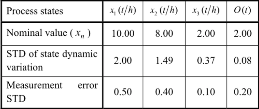
Table 4-1: Nominal values and standard deviations (STD) of model parameters. ... 77

Table 4-2: Transfer functions of the process model. ... 78

Table 4-3: Results for the estimation of nominal values with different window widths ... 79

Table 4-4: Estimation results of the dynamic process states. ... 80

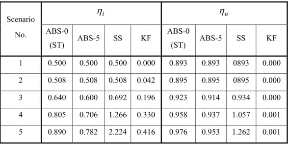
Table 5-1: Different simulation scenarios. ... 98

Table 5-2: Transfer functions of the separation unit. ... 99

Table 5-3: for the ABS observer with different time lags in Scenario 5 (separation unit). .... 99

Table 5-4: Variance reduction for SS, ABS and KF observers (separation unit). ... 100

Table 5-5: and for SS, ABS and KF observers in different scenarios (separation unit). ... 102

Table 5-6: Transfer functions of the flotation circuit. ... 103

Table 5-7: for the ABS observer with different time lags in Scenario 5 (flotation circuit). .. 104

Table 5-8: Variance reduction for SS, ABS and KF observers (flotation circuit). ... 105

Table 5-9: and for SS, ABS and KF observers (flotation circuit). ... 106

Table 5-10: and for the robustness test (_x₁ = 15 %). ... 107 i i P_, l t  _u i i P_, l t  _u t  _u

(14)

xiv

Table 5-11. Normalized indices for the robustness test (_x₁ = 15 %). ... 108

Table 6-1: Transfer functions of the separation unit model. ... 116

Table 6-2: Model parameters and uncertainties to be estimated. ... 120

Table 6-3: List of the estimated model parameters and uncertainties. ... 128

Table 6-4: Estimation of feed model characteristics. ... 128

Table 6-5: Performance indices (%) for ST, ABS, and KF observers. ... 131

Table 6-6: Performance indices (%) of ST, ABS, and KF in the robustness test. ... 132

Table 7-1: Process variables notations and units. ... 139

Table 7-2: Particles distribution in the feed. ... 141

Table 7-3: Value of function (Eq. 7-7) representing the distribution of the kinetic constant based on the particle size and composition. ... 145

Table 7-4: Summary of empirical relationships. ... 151

Table 7-5: Distribution of entrainment constants. ... 153

Table 7-6: Simulation algorithm details. ... 156

Table 7-7: Nominal value of cell dimensions, feed characteristics, and manipulated variables. .... 157

Table 7-8: Characteristics of particles distribution in the cell feed. ... 157

Table 7-9: Steady-state value of plant variables at the nominal operating regime. ... 158

Table 7-10: Maximum theoretical recovery-grade: species elimination order and recovery-grade calculation. ... 159

Table 7-11: Disturbances in the feed characteristics used to investigate cell steady-state performance. ... 162

Table 7-12: Different simulation scenarios based on the manipulated variables variations. ... 163

Table 7-13: Different simulation scenarios based on the feed characteristics variations. ... 176

Table 7-14: Characteristics of feed particles distribution for the grade variation scenarios. ... 180

Table 7-15: Flotation circuit - cell dimensions. ... 186

Table 7-16: Nominal value of feed characteristics and manipulated variables. ... 188

) , (d_i c_i g

(15)

xv

Table 7-17: Steady-state value of flotation circuit variables in the nominal operating regime. ... 188

Table 7-18: Flotation circuit: different simulation scenarios based on the manipulated variables variations. ... 189

Table 8-1: Manipulated and output variables list selected for APC and RTO design. ... 211

Table 8-2: Identified model transfer functions. ... 213

Table 8-3: APC objective function coefficients. ... 218

Table 8-4: RTO objective function coefficients. ... 222

Table 8-5: Coefficients of economic gain function. ... 231

Table 8-6: APC performance: disturbance 1 (feed rate & grade variation with constant liberation and middling grade) and all variables measured. ... 233

Table 8-7: APC performance: disturbance 1 (feed rate & grade variation with constant liberation and middling grade) and feed rate not measured. ... 236

Table 8-8: APC performance: disturbance 2 (feed rate & grade variation with non-constant liberation and middling grade) and all variables measured. ... 237

Table 8-9: APC performance: disturbance 2 (feed rate & grade variation with non-constant liberation and middling grade) and feed rate not measured. ... 238

Table 8-10: APC performance: disturbance 3 (stationary variation in solid percentage of feed rate) and all variables measured. ... 239

Table 8-11: APC performance: disturbance 3 (stationary variation in solid percentage of feed rate) and feed rate not measured. ... 240

Table 8-12: RTO performance: disturbance 1 (feed rate & grade variation with constant liberation and middling grade) and all variables measured. ... 244

Table 8-13: RTO performance: disturbance 1 (feed rate & grade variation with constant liberation and middling grade) and feed rate not measured. ... 247

Table 8-14: RTO performance: disturbance 2 (feed rate & grade variation with non-constant liberation and middling grade) and all variables measured. ... 248

Table 8-15: RTO performance: disturbance 2 (feed rate & grade variation with non-constant liberation and middling grade) and feed rate not measured. ... 249

(16)

xvi

Table 8-16: RTO performance: disturbance 3 (stationary variation in solid percentage of feed rate) and all variables measured. ... 250 Table 8-17: RTO performance: disturbance 3 (stationary variation in solid percentage of feed rate) and feed rate not measured. ... 251

(17)

xvii

List of Figures

Fig. 2-1: Single node separation unit. ... 14

Fig. 2-2: Inventory of a separation unit under different operating regimes (ton). ... 14

Fig. 2-3: Components of a state variable in stationary regime. ... 15

Fig. 3-1: Combustion chamber scheme. ... 41

Fig. 3-2: Case-study I: estimates vs. raw measurements. ... 45

Fig. 3-3: Case-study I: precision of estimated variables vs. optimum estimation. ... 46

Fig. 3-4: Hydrocyclone scheme. ... 47

Fig. 3-5: Case-study II: estimates vs. raw measurements (scenario 2). ... 50

Fig. 3-6: Case-study II: variables estimation precision vs. optimum estimation (scenario 2). ... 50

Fig. 3-7: Flotation circuit flow sheet. ... 52

Fig. 3-8: Case-study III: estimates vs. raw measurements. ... 54

Fig. 3-9: Case-study III: variables estimation precision vs. optimum estimation. ... 54

Fig. 3-10: Single node separation unit flow sheet. ... 57

Fig. 3-11: Case study IV: precision of the estimations vs. raw measurements. ... 58

Fig. 3-12: Case study IV: precision of the estimations vs. optimum estimation. ... 59

Fig. 3-13: Case-study V: Monte-Carlo simulation results for tuning (range 0.3 to 3)... 60

Fig. 3-14: Case-study V: Monte-Carlo simulation results for tuning (range 0.7 to 1.3). ... 60

Fig. 3-15: Case study V: precision of the estimations vs. raw measurements. ... 61

Fig. 3-16: Case study V: precision of the estimations vs. optimum estimation. ... 62

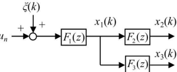
Fig. 4-1: A single node plant. ... 75

Fig. 4-2: Data preprocessing for dynamic data reconciliation by steady-state reconciliation software (data synchronization method). ... 76

Fig. 5-1: Single node separation unit. ... 89

Fig. 5-2: Complete causal dynamic model of the single node separation unit. ... 90 v



v

(18)

xviii

Fig. 5-3: Node imbalance autocovariance function of the separation unit. ... 92

Fig. 5-4: Performance indices as a function of in Scenario 5 (separation unit). ... 101

Fig. 5-5: Flotation circuit flow diagram. ... 102

Fig. 5-6: Performance indices as a function of in Scenario 5 (flotation circuit). ... 105

Fig. 6-1: Separation unit flow diagram... 115

Fig. 6-2: Separation unit model. ... 115

Fig. 6-3: Measurement autocovariance function. ... 123

Fig. 6-4: Iterative approach to estimate the feed model parameters and corresponding uncertainties. ... 124

Fig. 6-5: Flotation circuit flow sheet. ... 125

Fig. 6-6: Stationary variation of the valuable mineral feed rate. ... 126

Fig. 6-7: Distribution of time constants (Tc, Tr), poles (a2, a3) and separation coefficient ( ). ... 127

Fig. 6-8: KF and ST estimates vs. true and measured values (concentrate and reject flowrates). .. 131

Fig. 7-1: Flotation cell scheme. ... 139

Fig. 7-2: Mineral hydrophobicity and collector concentration relationship. ... 146

Fig. 7-3: and frother concentration relationship. ... 148

Fig. 7-4: Schematic of operational variables effect on the flotation rate constant and gas hold-up.151 Fig. 7-5: Flotation cell simulation algorithm. ... 155

Fig. 7-6: Flotation cell maximum theoretical recovery-grade curve. ... 160

Fig. 7-7: Cell recovery during the batch test. ... 161

Fig. 7-8: Cell steady-state recovery-grade for different feed disturbances. ... 163

Fig. 7-9: Flotation cell: variations of the manipulated variables. ... 164

Fig. 7-10: Cell performance: effect of the collector concentration on the flotation rate constant. .. 166

Fig. 7-11: Cell performance: the collector concentration effect on the output variables. ... 166

Fig. 7-12: Cell performance: froth depth when the collector concentration varies. ... 167

Fig. 7-13: Cell performance: plant recovery and grade when collector concentration varies. ... 167

l



32 D

(19)

xix

Fig. 7-14: Cell performance: frother concentration effect on the flotation rate constant. ... 168

Fig. 7-15: Cell performance: frother concentration effect on the output variables. ... 169

Fig. 7-16: Cell performance: froth depth when frother concentration varies. ... 169

Fig. 7-17: Cell performance: plant recovery and grade when frother concentration varies. ... 170

Fig. 7-18: Cell performance: air flowrate effect on the flotation rate constant. ... 171

Fig. 7-19: Cell performance: air flowrate effect on the output variables. ... 172

Fig. 7-20: Cell performance: froth depth when air flowrate varies. ... 172

Fig. 7-21: Cell performance: plant recovery and grade when air flowrate varies. ... 173

Fig. 7-22: Cell performance: the collection zone level effect on the flotation rate constant. ... 174

Fig. 7-23: Cell performance: froth depth when the collection zone level varies. ... 174

Fig. 7-24: Cell performance: the collection zone level effect on the output variables. ... 175

Fig. 7-25: Cell performance: plant recovery and grade when the collection zone level varies. ... 175

Fig. 7-26: Flotation cell: variations of the feed characteristics. ... 177

Fig. 7-27: Cell performance: feed rate changes effect on the output variables. ... 178

Fig. 7-28: Cell performance: plant recovery and grade when feed rate changes. ... 178

Fig. 7-29: Cell performance: froth depth when feed rate changes. ... 179

Fig. 7-30: Cell performance: feed rate changes effect on flotation rate constant... 179

Fig. 7-31: Cell performance: feed grade changes effect on the output variables. ... 181

Fig. 7-32: Cell performance: plant recovery and grade when feed grade changes. ... 182

Fig. 7-33: Cell performance: feed grade changes effect on flotation rate constant. ... 182

Fig. 7-34: Cell performance: froth depth when feed grade changes. ... 182

Fig. 7-35: Flotation cell: stationary variations of the feed characteristics. ... 183

Fig. 7-36: Cell performance: stationary variation of the feed characteristics effect on the output variables. ... 184

Fig. 7-37: Cell performance: plant recovery and grade when the feed characteristics stationary change. ... 185

(20)

xx

Fig. 7-38: Cell performance: stationary variation of the feed characteristics effect on the flotation

rate constant. ... 185

Fig. 7-39: Cell performance: froth depth when stationary changes occur in the feed characteristics. ... 186

Fig. 7-40: Flotation circuit flow diagram. ... 186

Fig. 7-41: Flotation circuit: variations of the manipulated variables. ... 190

Fig. 7-42: Circuit performance: the collector concentration effect on the output variables. ... 191

Fig. 7-43: Circuit performance: plant recovery-grade when the collector concentration varies. .... 192

Fig. 7-44: Circuit performance: the rougher collection zone level changes effect on the output variables. ... 193

Fig. 7-45: Circuit performance: plant recovery-grade when rougher collection zone level changes. ... 193

Fig. 7-46: Circuit performance: cleaner collection zone level changes effect on the output variables. ... 194

Fig. 7-47: Circuit performance: plant recovery-grade when cleaner collection zone level changes. ... 195

Fig. 7-48: Circuit performance: scavenger collection zone level changes effect on the output variables. ... 196

Fig. 7-49: Circuit performance: plant recovery-grade when scavenger collection zone level changes. ... 196

Fig. 7-50: Circuit performance: water addition changes effect on the output variables. ... 197

Fig. 7-51: Circuit performance: plant recovery-grade when water addition in cleaner feed changes. ... 198

Fig. 8-1: Typical control hierarchy. ... 202

Fig. 8-2: General control scheme. ... 208

Fig. 8-3: Flotation circuit schematic and location of selected variables. ... 211

Fig. 8-4: Identified transfer functions and plant data comparison. ... 214

(21)

xxi

Fig. 8-6: Step response of model TFs (APC scheme). ... 217

Fig. 8-7: APC performance test: controlled variables. ... 220

Fig. 8-8: APC performance test: manipulated variables. ... 220

Fig. 8-9: RTO performance test: step disturbance in the feed rate and composition. ... 223

Fig. 8-10: RTO performance test: manipulated variable. ... 223

Fig. 8-11: RTO performance test: output variables. ... 224

Fig. 8-12: Block diagram of DR coupled with APC and RTO loops. ... 225

Fig. 8-13: Flow sheet of the flotation circuit simulator used as the plant. ... 226

Fig. 8-14: Disturbance 1: variation in feed rate and grade (constant liberation & middling). ... 228

Fig. 8-15: Disturbance 2: variation in feed rate and grade (non-constant liberation & middling). 228 Fig. 8-16: Disturbance 3: variation in solid percentage (constant grade and particle population). 229 Fig. 8-17: Grade violation penalty function. ... 231

Fig. 8-18: APC: histogram of controlled and manipulated variables – Scenario 1 (without noise). ... 234

Fig. 8-19: Histogram of controlled and manipulated variables - Scenario 2 (with noise & without DR). ... 234

Fig. 8-20: APC: histogram of controlled and manipulated variables - Scenario 3 (with noise & with DR). ... 235

Fig. 8-21: APC: collector concentrate - without and with measurement noise. ... 243

Fig. 8-22: RTO: histogram of controlled and manipulated variables – Scenario 1 (without noise). ... 245

Fig. 8-23: RTO: histogram of controlled and manipulated variables - Scenario 2 (with noise & without DR)... 246

Fig. 8-24: RTO: histogram of controlled and manipulated variables - Scenario 3 (with noise & with DR). ... 246

(22)

(23)

xxiii

Acknowledgements

I would like to express my deepest appreciation and thanks to my advisors Professors Éric Poulin and Daniel Hodouin, for their excellent supervision and priceless guidance during all stages of my work. I would like to thank you for your endless supports and encouragements during these past five years. Working with you was a great honor and experience for me, and I will never forget it.

Moreover, I would like to thank jury members, Dr. Daniel Sbarbaro, Dr. André Desbiens, and Dr. Claude Bazin, for their valuable time that they spent for reviewing my thesis and for their professional comments and insightful guidance. I would also like to thank Dr. Luc Lachance for his professional supports during my Ph.D. project.

A special thanks to my family. Words cannot express how grateful I am to my parents, Gholam and Heshmat, my brothers, Amirabbas and Saeed, and my sister, Mina, for all of the sacrifices that you have made on my behalf. Your supports have been invaluable, and I owe you forever.

I am also very thankful to my great friends and my office mates especially Dr. Massoud Ghasemzadeh-Barvarz, Dr. Ali Vazirizadeh, Alberto Riquelme Diaz, Yanick Beaudoin, Mona Roshani, Mousa Javidani, Mahdi Amiriyan, Asria Afshar Taromi, Ali Shamsaddinlou, Dr. Amir Ghasdi, Saghar Tahmasbi, and Parnian Oktaie for their academic advices and personal supports.

Finally, I would like to express my appreciation to my friend and beloved wife Asra for her patience and kindness. She has always supported me emotionally and mentally when I get stuck or need reclusion. Without her, this project would never have been accomplished. I dedicate this thesis to my wife and my family.

(24)

(25)

xxv

Foreword

This thesis consists of 9 chapters and two appendices. The first chapter provides a general introduction to data reconciliation techniques, applications, issues, and objective of the study. In Chapter 2, the necessary background to understand and apply the data reconciliation techniques is presented. Chapters 3 to 6 are based on published or submitted articles in international scientific journals and conferences. Chapter 7 presents phenomena based simulator development of flotation circuits. In Chapter 8, value of data reconciliation coupled with advanced process control and real-time optimization schemes are investigated. Chapter 9 contains thesis conclusions and recommendations for future works.

Chapter 3:

Chapter 3 presents the importance of correctly tuning of the statistical properties of the modeling and measurement uncertainties in steady-state data reconciliation. It reveals that neglecting the covariance terms, which is a common industrial practice, and also incorrect tuning of variance terms of the uncertainties matrices can deteriorate the observer performance. In this chapter, using five case-studies taken from mineral and metallurgical industries, the following topics are studied:

 importance of considering the model parameter errors and their correlation terms  impact of taking into account the correlation of the measurement errors

 importance of involving process dynamic fluctuations in data reconciliation

 linearization of bilinear data reconciliation constraints and correctly tuning of corresponding measurement error covariance matrix

 impact of the variance terms of the uncertainties matrix on data reconciliation performance

(26)

xxvi

Amir Vasebi, Éric Poulin & Daniel Hodouin (2014), Selecting proper uncertainty model for steady-state data reconciliation – Application to mineral and metal processing industries. Minerals Engineering, 65, p. 130–144.

In this part of the project, I

 reviewed the related literature

 developed simulators for the case-studies in collaboration with my professors  developed a new technique to calculate the measurement error covariance matrix for

bilinear data reconciliation problems

 wrote the necessary MATLAB codes and built Simulink models  implemented the data reconciliation observers

 defined different simulation scenarios to investigate the effect of uncertainty covariance matrix on the performance of steady-state data reconciliation observer  analyzed and discussed the results in collaboration with my professors

 wrote the article manuscript in collaboration with my professors

Chapter 4:

Chapter 4 provides several techniques to apply the steady-state data reconciliation commercial software packages for dealing with process dynamics. It proposes three solutions. First, when unit inventories are measured, it is possible to use a sub-optimal implementation of data reconciliation with dynamic mass or energy conservation methods. In the second technique, plant input variables are pre-filtered for synchronizing with other plant variables, in such a way that steady-state reconciliation can be applied. Then, the dynamic process inputs are reconstructed. In the third option, fictitious streams representing the accumulation rate variables (node imbalances) are added to the plant network.

This work is presented in:

Daniel Hodouin, Amir Vasebi & Éric Poulin (2012), How to adequately apply steady-state material or energy balance software to dynamic metallurgical plant data. IFAC Workshop on Automation in the Mining, Mineral and Metal Industries, Gifu, Japan.

(27)

xxvii In this chapter, I

 worked on the mathematical development of the solutions in collaboration with my professors

 wrote the necessary MATLAB codes and built Simulink models  developed simulators for the case-studies

 implemented the data reconciliation observers

 defined different simulation scenarios in collaboration with my professors  analyzed and discussed the results in collaboration with my professors  wrote the article manuscript in collaboration with my professors

Chapter 5:

Chapter 5 introduces a new dynamic data reconciliation observer based on a mass conservation sub-model. The observer uses the autocovariance of node imbalances as additional information that improves the estimation precision. For evaluation purpose, two simulated benchmark plants operating in a stationary regime are used, and its performance is compared with classical sub-model based observers and Kalman Filter. The proposed observer provides more precise estimates than steady-state and standard stationary observers, particularly when the process dynamic regime becomes important compared to measurement errors. It exhibits more robust performances against modeling errors compared to Kalman filter. Although Kalman filter leads to optimal performances when perfectly tuned, it is more sensitive to modeling errors than the proposed observer.

This work is presented in:

Amir Vasebi, Éric Poulin & Daniel Hodouin (2012), Dynamic data reconciliation based on node imbalance autocovariance functions. Computers and Chemical Engineering, 43, p. 81–90.

(28)

xxviii

 carried out the mathematical development of the proposed observer

 developed simulators for the case-studies in collaboration with my professors  wrote the necessary MATLAB codes and built the Simulink models

 implemented the data reconciliation observer

 defined different tests, simulation scenarios, and performance evaluation indices  analyzed and discussed the results in collaboration with my professors

Chapter 6:

Chapter 6 proposes a procedure to obtain a simple model for a flotation circuit to support the implementation of Kalman filter for dynamic data reconciliation. Using simplifying assumptions, first-order empirical transfer functions obtained from the plant topology, nominal operating conditions, and historical data are used to build the model for Kalman filter. The flotation circuit simulator introduced in Chapter 7 is employed as the case-study. To obtain the model parameters and corresponding uncertainties, practical guidelines are provided. The performance of Kalman filter is compared with two sub-model based observers using the total estimation error variance reduction index and a robustness test. Kalman filter with the empirical model provides more precise estimates than standard and autocovariance based stationary observers. But in the robustness test, sub-model based observers reveal slightly better performance than the implemented Kalman filter.

This work is submitted as:

Amir Vasebi, Éric Poulin & Daniel Hodouin (2015), Determining a dynamic model for flotation circuits using plant data to implement a Kalman filter for data reconciliation. Minerals Engineering, 83, 192-200.

In this chapter, I

 carried out the mathematical development of the modeling error covariance matrix tuning

(29)

xxix  proposed guideline to estimate the model parameters and uncertainties using plant

data in collaboration with my professors

 wrote the necessary MATLAB codes and built Simulink models  implemented the data reconciliation observers

 defined different tests, simulation scenarios, and performance evaluation indices  analyzed and discussed the results in collaboration with my professors

Chapter 7:

Chapter 7 develops a dynamic simulator of froth flotation circuit for designing and testing data reconciliation observers and automatic control strategies. This simulator is built based on dynamic mass balance equations and empirical relationships. Collection and froth zones are modeled as the perfect mixer and plug flow reactors. Flotation and entrainment phenomena are considered in the collection zone modeling. Species drainage from the froth zone into the collection zone is also modeled by modifying flotation rate constants. Collector and frother concentrations, collection zone level, and air flowrate are considered as manipulated variables. The performance of a single cell and a flotation circuit are assessed using different test cases and scenarios. The simulator is employed as the case study for data reconciliation observer and advanced controller design in Chapters 6 and 8, respectively.

In this chapter, I

 carried out the mathematical modeling of the flotation cell in collaboration with my professors

 developed the simulator in MATLAB and Simulink  defined different tests and simulation scenarios

 tested the simulator performance in collaboration with my professors  analyzed and discussed the results in collaboration with my professors  wrote a technical report in collaboration with my professors

(30)

xxx

Chapter 8:

Two advanced process control and real-time optimization schemes based on receding horizon internal model control are designed in Chapter 8. The aim is coupling dynamic data reconciliation with an advanced controller and a real-time optimizer, and showing its economic value. For this purpose, the flotation circuit simulator developed in Chapter 7 is employed as the benchmark plant. For the advanced controller, a standard quadratic reference tracking objective function is defined while real-time optimizer has an economic based cost function. Then, they are coupled with autocovariance based stationary data reconciliation observer presented in Chapter 5. To assess the effect of involving data reconciliation in closed loop process, several test cases and disturbances are applied. Performance and economic benefits of the advanced control and real-time optimization schemes with and without data reconciliation are investigated using statistical measures and an economic gain function.

In this study, I

 developed an advanced controller and a real-time optimizer in collaboration with my professors

 applied a mass conserving system identification method to obtain the process model  developed the necessary MATLAB codes and Simulink models

 implemented and integrated the data reconciliation observer with the plant

 defined different simulation scenarios and tests in collaboration with my professors  defined the closed loop performance evaluation indices in collaboration with my

professors

 tested the closed loop performance in collaboration with my professors  analyzed and discussed the results in collaboration with my professors  wrote a technical report in collaboration with my professors

(31)

xxxi

Appendices:

Appendix A provides complementary information about the case-studies used in Chapter 3 while Appendix B presents the mathematical calculations used in Chapter 5 to build the autocovariance based stationary observer.

(32)

(33)

1

Chapter 1 Introduction

This chapter first discusses the data reconciliation observers and their effectiveness to improve the accuracy and the reliability of plant data. Issues associated with data reconciliation applications are also presented. Moreover, objectives of this research, original contributions, and a list of publications are given in the following sections.

1.1 Data Reconciliation

Efficient, profitable, and safe plant operations depend on accurate and reliable process data in mineral and metal processing plants. Measurement errors affecting variables such as chemical species concentration and/or particle size distribution are usually important due to sampling errors and material heterogeneity (Gy, 1982). Due costs associated with instrumentation and maintenance and/or technical concerns, direct measurement of such variables using on-line analyzers is faced with many limitations. On the other hand, taking samples with off-line techniques, i.e. laboratory analysis, is also time-consuming and expensive. Therefore, only necessary physicochemical variables and properties are usually measured and evaluated. These issues lead to inconsistency between measurements and process models, and also key properties of the material that are unmeasured.

Data reconciliation is considered as an effective technique to improve the accuracy and reliability of plant data. It is normally formulated as an optimization problem minimizing the measured and estimated variables difference while respecting constraints imposed by the process model. Mass and energy conservation equations are used as process constraints. The technique was first proposed by Kuehn and Davidson (1961) more than fifty years ago. Over time, many improvements and modifications were brought to the technique as

(34)

2

reflected by several reference works (Narasimhan and Jordache, 2000; Romagnoli and Sanchez, 2000; Puigjaner and Heyen, 2006). Data reconciliation has been recently revisited, and interesting mathematical interpretations have been suggested by Mistas (2010) and Maronna and Arcas (2009).

Usually, data reconciliation is coupled with complementary methods that take advantage of improved state estimations. It has been involved in many applications like process monitoring (Martini et al., 2013), plant simulation (Reimers et al., 2008), basic and advanced process control (Bai and Thibault, 2009) or real-time optimization (Manenti et al. 2011). In mineral and metal processing plants, data reconciliation has been widely applied in production accounting, survey analysis, sensor network design and fault detection (Hodouin, 2010; Narasimhan, 2012; Berton and Hodouin, 2003; Berton and Hodouin, 2007).

A wide range of models ranging from simple sub-models like steady-state mass/energy conservation constraints to a complete dynamic causal model has been proposed to handle the plant dynamics for data reconciliation purpose. A model built based on detailed and accurate information about process behavior leads to more precise estimations than those obtained from simple process models. In practice, developing and calibrating such models are demanding tasks. Hodouin (2011) has discussed and presented this point for mineral and metal processing plants.

The simplest approach is to average data to attenuate dynamic variations and apply steady-state data reconciliation (Bagajewicz and Jiang, 2000). Due to its simplicity, this technique is commonly used in numerous industry applications (Bagajewicz, 2010). The approach provides good results when processes have small dynamic variations, but for highly dynamic regimes, estimates could be less precise than measurement themselves (Almasy, 1990; Poulin et al., 2010)

Stationary data reconciliation was proposed by Makni et al. (1995a, 1995b) and Vasebi et al. (2012a) to handle plant dynamics with limited modeling efforts. These techniques consider inventory variations as random variables and rely on the autocovariance function of node imbalances. Other studies have also combined material conservation constraints

(35)

3 with inventory measurements to deal with dynamic variations. These studies can be grouped into two categories: generalized linear dynamic observers (Darouach and Zasadzinski, 1991; Rollins and Devanathan, 1993; Xu and Rong, 2010) and integral linear dynamic observers (Bagajewicz and Jiang, 1997; Tona et al., 2005). However, assuming the availability of inventory measurements is an important limitation. For instance, in the mineral processing industries, measuring of the inventory for a particular species in a separation unit is very difficult or almost impossible.

In the presence of a dynamic causal model of the process, Kalman filter (Kalman, 1960) is largely used to solve dynamic data reconciliation problems (Narasimhan and Jordache, 2000). Approaches inspired by Kalman filter such as the predictor-corrector-based algorithm (Bai et al., 2006) or the generalized Kalman filter (Lachance et al., 2006a) also represent interesting alternatives. However, obtaining the required process models for these algorithms implementation could be difficult and laborious in practice.

In mineral and metal processing industries, data reconciliation is well-established and widely applied. Mass and energy conservation constraints are usually applied as the process model to estimate the underlying steady-state values of process variables. Total material, as well as species flowrates, are estimated leading to bilinear data reconciliation problems. In the Gaussian context, a Maximum-Likelihood estimator is retained. Typically, it is assumed that measurement errors are unbiased and uncorrelated. To characterize the measurement errors, corresponding covariance matrices are often tuned using approximate techniques or trial and error approaches without paying attention to the impacts on the precision of estimated process variables.

1.2 Problem Statement

Data reconciliation is based on a trade-off between modeling effort and estimates precision. In general, model built based on detailed and accurate information of process results in more precise estimations than those that are estimated using the simple description of process models. However, as mentioned before, developing, calibrating, and maintaining such models are challenging tasks in practice (Hodouin, 2011). Using inadequate and inappropriate dynamic models with highly uncertain parameters could also lead to biased

(36)

4

estimates (Dochain, 2003; Özyurt and Pike, 2004). These considerations have often led to the use of simple but reliable sub-models instead of complex and detailed models involving uncertain parameters. The desire of finding a suitable compromise between modeling efforts and estimation performances motivate the development of new observers and development of procedures to obtain appropriate process models used in existing powerful observers like Kalman filter.

Moreover, the performance of data reconciliation observers strongly depends on the covariance matrices used to characterize the model and measurement uncertainties (Bavdekar et al., 2011). In some cases, inappropriate selection can even lead to divergence of the observation algorithm (Willems and Callier, 1992). In steady-state data reconciliation, measurement uncertainties evaluation techniques are generally based on direct methods (that only use measured process variables (Morad et al. 1999)) and indirect methods (which rely on process constraint residuals (Keller et al., 1992; Chen et al., 1997; Darouach, et al., 1989)). A tuning method based on covariance analysis to separate process fluctuations from measurement errors has been proposed by Lachance et al. (2007) for stationary observers. Regarding the evaluation of uncertainties for Kalman filter, several techniques have been introduced in the literature as illustrated by Dunik et al. (2009), Bavdekar et al. (2011), Dunik and Simandl (2008), and Akesson et al. (2008). Determining these covariance matrices is a crucial exercise that has to be carefully addressed to ensure a successful implementation of observers. Besides introducing new tuning techniques, investigation on the effect of uncertainty covariance matrices on the performance of data reconciliation observers is strongly in demand.

High-quality data is essential to make suitable decisions and consequently maximize profits, deal with market changes, and achieve technical objectives. Moreover, to maintain a plant around the optimum point, e.g. for advanced process control, real-time optimization, or plant supervision applications, data quality plays a critical role. Based on the literature, data reconciliation can generally improve the performance of control strategies and real-time optimization by attenuating the measurement noise variance and control action amplitude, estimation of unmeasured variables, updating model parameters, and improving model and data coherency. From an industrial point of view, these improvements can bring

(37)

5 better products quality and more economic revenues. A limited number of papers have coupled data reconciliation with process control (Ramamurthi et al., 1993; Abu-el-zeet et al., 2002; Zhou and Forbes, 2003; Bai et al., 2005a; Bai et al., 2007) and real-time optimization (Naysmith and Douglas, 1995; Zhang and Forbes, 2000; Faber et al., 2006; Hallab, 2010). Most of these studies have evaluated the data reconciliation effectiveness using statistical properties of manipulated and controlled variables, and/or some qualitative measures. They have not investigated the potential economic revenues obtained by applying data reconciliation. Therefore, at least a case-based study is required to reveal how much data reconciliation can be beneficial for a given plant from the economic point of view.

(38)

6

1.3 Objectives of this Work

As reflected by the literature on data reconciliation and as discussed in the problem statement section, there are several issues associated with the development, implementation, and application of data reconciliation observers in practice. To address these points, the aims of this study are:

 Investigating the effect of correctly selecting uncertainty covariance matrices, used for characterizing the modeling and measurement errors, on the data reconciliation performance.

 Developing new dynamic data reconciliation observers based on limited modeling efforts.

 Determining a simple dynamic model for mineral processing plants to support the implementation of a Kalman filter for data reconciliation purpose.

 Developing a simulator of the mineral processing plants for design and test of data reconciliation observers and process control strategies.

 Coupling data reconciliation observers with advanced process control and real-time optimization schemes, and consequently investigating the benefits of using data reconciliation in closed loop plants.

(39)

7

1.4 Original Contributions

Briefly, the main contributions of this thesis are:

 Classification of the data reconciliation observers based on target value estimation: steady-state underlying value versus the true value of variables.

 Proposition of a systematic technique to classify the different source of uncertainties (i.e. modeling errors, process dynamics, and sampling and analysis errors), and also correctly selecting of the uncertainties covariance matrices for steady-state data reconciliation purpose.

 Development of a new technique to calculate the measurement error covariance matrix for bilinear data reconciliation problems, in contrast with existing incorrect practices.

 Proposition of the recommendations and tricks to deal with plant dynamics using the available steady-state data reconciliation software.

 Development of a new stationary data reconciliation observer based on node imbalance autocovariance function.

 Proposition of a procedure to obtain a dynamic empirical model for a flotation circuit based on plant operation and design information for dynamic data reconciliation purpose using Kalman filter.

 Development of the new performance indices for comparing the different data reconciliation observers.

 Development of a phenomenological simulator for a flotation circuit used for design and test of data reconciliation observers and process control schemes.

 Integration of the data reconciliation observers with advanced process control and real-time optimization schemes for illustrating the economic value of using data reconciliation in a simulated flotation plant.

(40)

8

1.5 List of Publications

A list of published and submitted articles in journals and conferences obtained as a result of this research is presented below:

1) Vasebi, A., Poulin, É. & Hodouin, D. (2015), Determining a dynamic model for flotation circuits using plant data to implement a Kalman filter for data reconciliation. Minerals Engineering, 83, 192-200.

2) Vasebi, A., Poulin, É. & Hodouin, D. (2014), Selecting proper uncertainty model for steady-state data reconciliation. Minerals Engineering, 65, p. 130-144.

3) A Vasebi, A., Poulin, É. & Hodouin, D. (2012), Dynamic data reconciliation in mineral plants. Annual Reviews in Control, 36, p. 235-243.

4) Vasebi, A., Poulin, É. & Hodouin, D. (2012), Dynamic Data Reconciliation Based on Node Imbalance Autocovariance Functions. Computers and Chemical Engineering, 43, p. 81–90.

5) Vasebi, A., Hodouin, D. & Poulin, É. (2013), The importance of uncertainty covariance tuning for steady-state data reconciliation in mineral and metal processing. 15th IFAC Symposium in MMM, San Diego, USA.

6) Hodouin, D., Vasebi, A. & Poulin, É. (2012), How to adequately apply steady-state material or energy balance software to dynamic metallurgical plant data. IFAC MMM 2012, Gifu, Japan.

7) Vasebi, A., Poulin, É. & Hodouin, D. (2011), Observers for Mass and Energy Balance Calculation in Metallurgical Plants. 18th IFAC World Congress, Milano, Italy.

8) Vasebi, A., Poulin, É., Hodouin, D. & Desbiens, A. (2015), Coupling dynamic data reconciliation with model predictive control for real-time optimization of a flotation plant simulator. Submitted to XXVIII International Mineral Processing Congress (IMPC 2016), Québec City, Canada.

(41)

9

Chapter 2 Data Reconciliation: Background

This chapter presents the fundamental points that are necessary to understand and apply the data reconciliation techniques. First, accuracy and precision of a measurement are defined based on the different measurement error types. Then, various plant operating regimes are illustrated and discussed. Moreover, the target value of each process variable, i.e. the one that should be estimated by data reconciliation, is clearly stated. Different process models used in the data reconciliation observers, ranging from a simple mass conservation sub-model to a complete causal dynamic sub-model, are also shown in the chapter. Finally, to complete the presentation of process models, measurement equation of the process variables is presented.

2.1 Introduction

Accurate and reliable process data is needed to have an efficient, profitable, and safe plant operation. Plant-wide management and business strategies depend on performance indicators like productivity, material quality and production cost information that combine economic and technical factors. These factors are strictly related to the process variables such as production rate, metal recovery, product grade, and energy consumption. High-quality data is essential to make suitable decisions to maximize profits, deal with market changes, and achieve technical objectives. Moreover, to keep a plant around the optimum point, e.g. for advanced process control, real-time optimization, or plant supervision applications, data quality plays a critical role.

(42)

10

Presence of the random and gross errors in the measurements, infrequent laboratory analyses, and unmeasured strategic variables are the major concerns in most of mineral and metallurgical plants. For these processes, there are many unmeasured flowrates because of technical and economic issues. In contrast, the physical properties and the chemical content of flowing material are analyzed for a large number of streams. However, these analyses are subject to significant measurement errors associated with sampling errors (Pitard, 1993; Holmes, 2004) causing problems for advanced control and optimization applications. Data reconciliation (DR) is widely applied to improve the reliability and accuracy of data in mineral processing industries. It reduces impacts of random errors by producing estimates coherent with a process model and giving the possibility to estimate the unmeasured variables under favorable observability conditions. For the first time, Kuehn and Davidson (1961) have proposed data reconciliation based on Lagrange multipliers for the steady-state data reconciliation problem. As a proven technique, it has been largely applied to various industrial sectors such as chemical and biochemical processes (Dochain, 2003), pulp and paper industries (Bellec et al., 2007) and mineral and metallurgical processing (Hodouin, 2010). Over the years, many comprehensive books and papers describing fundamental aspects of data reconciliation have been presented (Narasimhan and Jordache, 2000; Romagnoli and Sanchez, 2000; Bagajewicz 2010; Puigjaner and Heyen, 2006; Crowe, 1996; Tamhane and Mah, 1985; Hlavacek, 1977; Mitsas, 2010; Maronna and Arcas, 2009). For successful implementation of data reconciliation observers, developing a process model is a crucial task. The representation of process model could range from simple noncausal sub-models, e.g. mass conservation constraints, to complete causal dynamic models. In general, more accurate and detailed process model would lead to more precise estimates while using simpler plant description produces less precise estimations. However, in practice, building and calibrating of detailed models is a challenging task (Hodouin, 2011). Updating and maintaining complex models is another point that could be problematic. All these factors have often motivated the use of simple sub-models that have high confidence level rather than complete but uncertain models. The trade-off between estimation performances and modeling efforts has led to different observers regarding the various types of models used to cope with process dynamics.

(43)

11 Plant operating regime is another factor that can affect the development and performance of the observers (Lachance et al., 2006b). Depending on how plant feed varies, the process model and observer structure could be different. Assuming steady-state operating regime, when feed largely fluctuates, could lead to much simpler observers with less precise estimates while developing observers that take into account the feed variations could result in better estimation.

Depending on which part of measured variables should be estimated by data reconciliation, observer design could be different. Each process variable, ignoring the measurement noises, can be represented by two components: a) local/underlying value and b) true value including the underlying value and dynamic variations. Both of these values can be targeted and estimated by data reconciliation observers. Estimation of the underlying value leads to steady-state observers while attempt to estimate the true value is called dynamic DR. Therefore when a data reconciliation observer is developed, the target value should be clearly mentioned.

As the main objective, the points that are necessary to understand and develop data reconciliation observers are presented in this chapter. These concepts are clearly defined for avoiding any confusion in the thesis. Section 2.2 is dedicated to present the various measurement errors, and consequently definition of the measurement accuracy and precision. Then, in Section 2.3, plant operating regimes are illustrated based on the inventory variations. Estimating the averaged underlying value or true dynamic value as the objective of DR is extensively discussed in Section 2.4. Process models applied in DR observers, ranging from a simple mass conservation sub-model to a complete causal dynamic model, are shown in more details in Section 2.5. Finally, to complete the presentation of process models, Section 2.6 provides the measurement equation of the process variables.

(44)

12

2.2 Precision versus Accuracy

Measured data is always affected by errors related to measuring devices. No sensor can be built that is exact and accurate. Also, errors can arise from sampling or sensors positioning caused by the inherent space and time heterogeneity of process variables. About the source of errors in the measurements, a discussion is presented in Chapter 3. Narasimhan and Jordache (2000) have categorized the measurement errors into two main classes:

 Random errors: the random term implies that neither the magnitude nor the sign of the error can be predicted with certainty. In other words, if the measurement is repeated with the same instrument under identical process conditions, different values may be obtained depending on the outcome of the random error. The only possible way that these errors can be characterized is using probability distributions, a property that quantifies measurement precision. These errors can be caused by some different sources such as power supply fluctuations, network transmission and signal conversion noise, changes in ambient conditions, and so on. This error usually corresponds to the high-frequency components of a measured signal and is usually small in magnitude.

 Gross errors, including biases (systematic errors) and outliers, are caused by non-random events such as instrument malfunctioning (due to improper installation of measuring devices), miscalibration, wear or corrosion of sensors, and solid deposits. Therefore, their occurrence and magnitude have not any random distribution. The non-random nature of these errors implies that, at any given time, they have a certain magnitude and sign that are usually unknown.

Based on the presented error classification, the accuracy of a measurement is defined as the closeness to the true value and it includes the effect of both gross and random errors (Miller, 1983). From a mathematical point of view, Mean-Square Error defined as the expected value of the square of the deviation between the estimated and the true value can be a representative for the measurements accuracy. While precision stands for the scattering of samples, i.e. measurements, around the samples mean which could be different from true value. In this sense, standard deviation σ can be an indication of the measurement

(45)

13 precision. The smaller value of σ implies more precision on the measurement and the higher probability that the random error can be close to zero (Benqlilou, 2004). When no bias is present, accuracy and precision are equivalent.

2.3 Plant Operating Regimes

To implement appropriate DR observers, characterization of the process operating regime is an essential factor. The variation of process states mainly depends on the plant dynamics, production rate changes, and the nature of disturbances. Using the node imbalances as a criterion for operating regime classification, four categories could be proposed (Lachance et al., 2006b):

 The steady-state regime: this regime assumes that all process inventories are constant; it implies a zero node imbalance at any time. Based on this definition, flowrates are allowed to fluctuate when equipment related to process nodes have fixed inventories or very fast time response compared to the stream dynamics.  The stationary operating regime: in practice, a strictly steady-state regime with

constant inventory is never met. There are always random or deterministic dynamic variations that can be small or quite significant. The stationary operating regime assumes that, over a long period of time, the process stream properties as well as inventories randomly vary around a constant value with positive and negative values. This operating mode is more realistic than the steady-state regime, and it can be applied to represent a wide range of industrial processes that operate in normal conditions during sufficiently long periods where major deterministic changes do not occur.

 The transient regime: when a process goes from one operating point to another one. On a short time window, to make a distinction between a stationary operating regime and a transient operating condition is a difficult task.

 The quasi-stationary regime: it is a combination of both stationary and transient operating conditions where the stationary intervals are significantly longer than the transient ones. In this mode, the process evolves from one stationary condition to another.

(46)

14

To illustrate the classification, Fig. 2-1 introduces a single node separation unit. The inventory of this process is shown in Fig. 2-2 for different regimes. Local stochastic variations (high frequencies) are mainly caused by input disturbances while trends (low-frequency variations) are the consequences of the deterministic abrupt or slow changes in the input variables. In this thesis, it is assumed that plants always operate in the stationary regime that is a reasonable assumption from the industrial point of view.

Fig. 2-1: Single node separation unit.

Fig. 2-2: Inventory of a separation unit under different operating regimes (ton).

Feed Concentrate Reject 0 500 1000 1500 2000 2500 3000 3500 4000 4500 5000 1 2 3 Inve nt or y Steady-state 0 500 1000 1500 2000 2500 3000 3500 4000 4500 5000 1 2 3 Ii nve nt or y Stationary 0 500 1000 1500 2000 2500 3000 3500 4000 4500 5000 1 2 3 Time (minute) Inve nt or y Quasi-stationary 0 500 1000 1500 2000 2500 3000 3500 4000 4500 5000 1 2 3 Inve nt or y Transient

(47)

15

2.4 Process State Variable versus Steady-State Underlying Value

Feed fluctuations, either random or dynamic, cause dynamic variations in the process states . Under stationary operating regime assumption, at least for a sufficiently long operating time, each process state fluctuates around a mean value , therefore allowing to define a dynamic deviation (Fig. 2-3). Defining as the averaged value of a process variable in the time window of samples, its variation tends to zero when h becomes larger and it has the maximum variance when h=1 . In general, does not perfectly obey the steady-state mass or energy conservation law, the deviation becoming smaller for larger

.

Fig. 2-3: Components of a state variable in stationary regime.

x x xm m d x x x   x_h x h h x h 0 50 100 150 200 9 10 11 Fl ow ra te ( t/h )