Quantile regression with a metal oxide sensors array for methane prediction over a municipal solid waste treatment plant

Quantile regression with a metal oxide sensors array for methane prediction

over a municipal solid waste treatment plant

Eric Martial TAGUEMa*_{, Luisa MENNICKEN}a_{, Anne-Claude ROMAIN}a Abstract:

Methane leakage is a crucial issue regarding its potential Green House effect. This study developed a quantile regression model for methane estimation over a municipal solid waste treatment plant (MSW) subject to biogas leakages and monitored with MOS gas sensors. Experimental data from 6 MOS gas sensors and a methane FID analyser taken during fourth months have been used for that purpose. The data processing consisted of (i) a drift correction, (ii) the addition of interactions, (iii) a principal component analysis (PCA) to extract new uncorrelated predictors, and (iv) a log transform of the methane data distribution. The forecast ability of the derived field calibrated model, compared with results from PLS regression, indicates well how helpful has been the data processing methods. Moreover, it highlighted, with some caution, the interest in using the quantile regression and interactions for models with MOS gas sensors considering the cross-sensitivity.

Keywords: MOS sensors; Quantile regression; Interactions; Cross-sensitivity.

a _{University of Liège, Faculty of Sciences, Department of Environmental Science and Management -} Sensing of Atmospheres and Monitoring (SAM) - Avenue de Longwy 185, 6700 Arlon (Belgium). * Corresponding author: emtaguem@uliege.be (Eric Martial TAGUEM)

1. Introduction

Methane is one of the major greenhouse gases considering its contribution to global warming over 100 years [1]. Nowadays, monitoring of methane has become essential with the ongoing climate change issue, and it is widely done by reference methods (e.g. eddy covariance, methane gas analysers, optical methane gas analysers [2]). However, the spatial coverage of these methods remains a limit considering the cost, technical skills required in addition to logistical challenges. New approaches involving the use of low-cost gas sensors can be helpful since they might expand the spatial resolution [3–5]. For example, several devices based on low-cost sensors and arranged as networks for continuous measurements can enhance spatial resolution and temporal resolution [6].

Besides the extensive use in the monitoring of air pollutants such as nitrogen oxides (NOx), carbon monoxide (CO) with low-cost electrochemical sensors, low-cost metal oxide semiconductors (MOS) gas sensors have been used for field monitoring in both quantitative and qualitative approaches (e.g. electronic nose for odour pattern recognition but also in device for methane determination [3,6]). It has been noted that for a quantitative approach with MOS gas sensors, laboratory calibrated model showed promising results, but the predictive performance becomes poor out of the laboratory [7]. In the context of field application, the cross-sensitivity of MOS gas sensors, the signal drift[8] and local environmental factors have been reported as the main reasons for inconsistency of predictive models derived from laboratory calibration [9]. In the same manner, predictive models derived from field calibration approaches also suffer from MOS sensors cross-sensitivity or changes in environmental factors. It is a concern that needs investigation.

In recent years, there has been a growing interest in using complex algorithms for model calibration on data from MOS gas sensors. Besides the traditional approaches based on multi-linear regression or partial least square regression [10,11], complex algorithms from machine learning as neural network or support vector machine regression have been used with promising results [12,13]. Machine learning provides a wide range of useful tools for data mining. However, the choice of appropriate tools regarding predictive performance, the model complexity, and interpretability are key challenges. For instance, sophisticated methods lead to black-box models with difficulties in linking model terms with a physical phenomenon. On the other hand, simple approaches as linear regression remain the best way to avoid overfitting and give

a better chance for generalisation. However, they might suffer from the presence of a significant bias on prediction [14].

Multiple linear regression also called Ordinary Least Squares (OLS) regression, as it is based on minimising the sum of squares of residuals, is the methodology widely used to describe the relationship between a dependent variable (target) and a subset of independent variables (predictors). However, OLS regression is subject to several assumptions (linearity, heteroscedasticity, normal distribution of errors, no autocorrelation). If one of them is violated, the prediction may become questionable. Beside the OLS regression, the quantile regression (QR) introduced by Koenker and Basset [15] has become a matter of interest. It is based on minimising the least absolute deviation (LAD), robust against outliers and interesting for dealing with non-normal data distribution and tailed distributions [16,17].

In this article, we propose to explore the development of a QR predictive model for field methane concentration from a dataset presenting the consideration mentioned above (drift, cross-sensitivity, environmental factors effects, non-normal data distribution). We also investigate predictive ability and the limits of the use of the final derived model. The final methodology will be used to develop a model with new or other MOS gas sensors that could be used with a ground mobile robot or a drone for field monitoring. 2. Material and methods

2.1 Experimental site description

The data were recorded on a MSW plant located in a rural area in Belgium. Because of a non-disclosure agreement, we cannot give its localisation. The MSW is over 50 ha in size and houses several economic activities in addition to biogas production. Due to unwanted CH4 leakages from the waste disposal site, the surrounding area was expected to show a significant increase of methane mixing ratio in the air at certain moments.

2.2 Instruments

Two devices installed in a mobile laboratory-called trailer- of the Institut Scientifique de Service Public (ISSeP) were used during the whole experimentation to monitor the biogas and methane concentration: a MOS sensors array device and a FID gas analyser. The MOS device has been designed by the ULiège "Sensing of Atmospheres and Monitoring" research unit. It contained six commercial gas sensors from Figaro® and UST® (TGS2602, TGS2610, TGS2611, TGS2620, GGS1330, TGS2444).

They have been selected knowing that MOS gas sensors show a slightly higher sensitivity to some compounds with respect to others and have a broad-ranged overlapping sensitivity. Consequently, we knew that our selected sensor array could show a response in the presence of biogas. The number of sensors has been limited to six, regarding the availability on the electronic board. A complete description of the device can be found in previous papers [18,19].

To measure methane concentration in ppmv, a Flame Ionisation Detector (FID), regularly calibrated following the European Ambient Air quality directive [2] was used. Commonly used in portable gas chromatographs, FIDs respond to the presence of methane and other hydrocarbon gases [20].

2.3 Data collection

The trailer from ISSeP was installed as close as possible to a location known to be subject to unwanted biogas leakages according to the prevailing wind and local topography relief. An air sampling probe at 2.8 m from the ground was used to collect the air above the mobile laboratory, and the same sampled air was driven to both measurement devices thanks to a "Tee" connection. The FID analyser's acquisition time was instantly and average to 30 minutes following the European Ambient Air directive [2]. The same was done with all gas sensors' resistance so that sensors and methane datasets can be paired. Data from both devices were recorded in internal memory and downloaded after.

2.4 Dataset Description

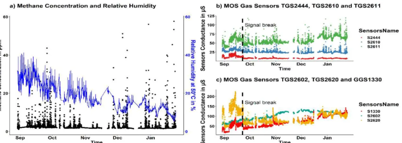
Fig. 1. a) Measurements of the CH4 concentration peaks and relative humidity. MOS gas sensor signals showing similar peaking are presented in the plot (b), and the sensors showing a signal drift are presented in the plot (c).

Data were collected from the end of August 2016 until the end of January 2017. For methane analyser, records started from the 24/08/2016 00:00:00 to 30/01/2017 while for MOS gas sensors they started from 29/08/2016 13:28:57 to 30/01/2017 23:55:13. Due to electrical issues and maintenance activities on mobile laboratory, no records were sometimes encountered on both datasets. They have been considered as missing values and removed. The remaining datasets were paired afterwards in one single dataset. Such that for one record, the following information was available: time (UTC zone format), MOS gas sensor conductance in microsiemens (µS), and methane mixing ratio in part per million (ppmv) (Fig. 1).

For this paper, the dataset was interesting in the light of all potential sources of variability observed on the evolution of MOS gas sensors signals. Fig. 1a and b show methane releases and MOS gas sensors responses (TGS2610, TG2612). Other interesting points are the break on sensors signals visible for instance, on TGS2620 signal (Fig. 1c) and a continuous conductance increase for four sensors (TGS2602, TGS2611, TGS2620 and GGS1330).

2.5 Data pre-processing and model set up

Sensors conductances (inverse of the resistance) recorded from the 6 MOS gas sensors have been taken as primary predictive variables and the measured CH4 concentration from FID analyser as a proxy for the real CH4 concentration. Methane concentration distribution appeared to be a tailed distribution because many records taking during a quiet period of activity over the MSW site showed a methane concentration values close to the background concentration. For regression, we considered the raw value and its log value (Fig. 2a).

We used the Iterative Restrictive Least Square method from Baseline package in R [21] to remove the drift observed on MOS gas sensors signals (Fig. 2b). The drift correction did not remove the signal break mentioned in the previous section. It is well illustrated in Fig. 2c by the change in variability of 2 sensors over three parts of the dataset (the first part before the break, the second part from October 2016 to December 2016 and the last part in January 2017). It should be understood as a change in response evolution due to unexplained external changes (not a drift!).

After applying the drift correction, we considered four configurations for the model designing by combining, or not, two modifications on model setup. The first one consisted of adding sensors interactions to take full variable possibilities (main effects and interactions), and the second one was the log transformation of [CH4] dataset.

Fig. 2. Density curves of [CH4] and log([CH4]). Median of each data distribution has been plotted in dashed line. b) Drift correction on MOS gas sensor GGS1330. c) Box plots of TGS2610 and TGS2620 sensors conductances over three parts of the dataset.

Because of the sensors' cross-sensitivity and non-specificity, their measurements often showed up the same trend simultaneously, as presented in Fig. 1b and c. The signal is then expected to be located in the combination of several sensors because they can react to a range of chemical compounds. The interaction term is defined here as a multiplication of sensors signals taken at the same time. Interactions up to the maximal order of 6, leading to 63 terms (Table 1), can be used as explanatory variables in the prediction model. These interactions enabled us to consider the effects of multiple sensors simultaneously.

Table 1. Main effect and interactions.

S2602 denoting the TGS2602 sensors data and S2602∙S2610 the interaction between S2602 and S2610.

Order Number of interaction Example of an interaction term

1 𝐶 = 6 S2602 2 𝐶 = 15 S2602∙S2610 3 𝐶 = 20 S2602∙S2610∙S2611 4 𝐶 = 15 S2602∙S2610∙S2611∙S2620 5 𝐶 = 6 S2602∙S2610∙S2611∙S2620∙S1330 6 𝐶 = 1 S2602∙S2610∙S2611∙S2620∙S1330∙S2444 Total 63

Once all pre-processing operations were made, Principal Component Analysis (PCA) has been done to get new uncorrelated variables before going through the model training process.

2.6. Quantile regression (QR)

The theoretical basis of the QR has been widely presented in several papers [15,16,22], and here we only showed the basic equations behind this particular approach of linear regression. Let (𝑋 , … , 𝑋 ) be a sample of a random variable 𝑋 with the distribution 𝐹. The empirical quantile of order τ is defined as 𝑄 (𝜏) = inf {𝑥 ∶ 𝐹 (𝑥) ≥ 𝜏}. For all 𝜏 ∈ [0,1], the loss function is defined by the following equation:

𝜌 (𝑥) = 𝑥 𝜏 − 𝟏(𝑥 < 0) ;

𝑤𝑖𝑡ℎ 𝟏(∙) 𝑡ℎ𝑒 "indicator function" 𝑔𝑖𝑣𝑖𝑛𝑔 𝜏𝑥 𝑖𝑓 𝑥 > 0 (𝜏 − 1)𝑥 𝑖𝑓 𝑥 < 0 (1)

Let ( 𝑥 , … , 𝑥 ) be n quantitative observations. The empirical quantile of order τ minimises the following objective function: 𝑉(𝜀) = ∑ 𝜌 (𝑦 − 𝜀) with 𝑦 the dependent variable of interest. For a given conditional quantile of order 𝜏, the model is written as a linear combination in terms of 𝑥 with a set of coefficients 𝛽 estimated by:

𝛽 = 𝑎𝑟𝑔𝑚𝑖𝑛( 𝜌 (𝑦 − 𝑥 𝛽 )) 𝑤𝑖𝑡ℎ 𝛽 ∈ 𝑅 (2)

The model (noted 𝑄𝑢𝑎𝑛𝑡 (𝑦 |𝑥 ) = 𝑥 𝛽 ) estimates the conditional quantile of order τ of the dependent variable (𝑦) given a set of predictors (𝑥). The quantile's coefficients (𝛽 ), for a given regressor 𝑗 associated to the 𝑗th element of 𝑥, should be interpreted as a marginal change in the 𝜏th _{conditional quantile} of 𝑦 given 𝑥 due to a marginal change in the 𝑗th _{variable [23]. A misguided idea from the name quantile} regression may emerge, but it does 𝒏𝒐𝒕 mean that regression is applied on a subsample of data or a quantile at all [24]. We want the reader to keep in mind its similarity with the classic linear regression.

2.7. The goodness-of-fit index (R1_{) and Cross-validation}

The goodness-of-fit index, for a given quantile of order 𝜏, is defined from the value of the objective function of the unrestricted model (𝑉 𝛽 ) and the restricted model (𝑉 𝛽 ). The restricted model being

defined with only the intercept (no predictor) [16]. 𝑅 (𝜏) = 1 − 𝑉 𝛽

𝑉 𝛽 (3)

𝑅 is an analogue of the criterion 𝑅 used in OLS regression. In contrast to the 𝑅 coefficient, it gives a local information because it is computed for each quantile [22].

The cross-validation was done by using dedicated functions proposed by the R package named rqPEN. This package performs the regularised regression called Least Absolute Shrinkage Selection Operation (LASSO). It consists of adding a constraint on the model coefficients thanks to a tuning parameter called lambda (𝜆) (see equation 4)[25].

𝛽 = 𝑎𝑟𝑔𝑚𝑖𝑛( 𝜌 𝑦 − 𝑥 𝛽 ) + 𝜆 |𝛽 | 𝑤𝑖𝑡ℎ 𝛽 ∈ 𝑅 (4)

The benefit of Lasso Penalization is that it is also a useful tool for making a model selection or reducing the number model equation terms. By changing the 𝜆 value, some coefficients are set to zero and therefore will not be considered in the final model equation. It is essential to reduce the number of predictors variables such that only the most relevant variables are kept in the final model allowing a more straightforward interpretation [26].

2.8 Model development, training and testing

We first performed a Principal Component Analysis (PCA) on the data set (raw data, raw data + interactions, raw data + interactions + drift correction) to study the dataset variability and the effects of pre-processing method (Section 3.1). After that, we investigated the QR model's quality considering data processing methods and selected quantiles 𝜏 = 0.1, 0.25, 0.5, 0.75 and 0.90 (Section 3.2). For that purpose, the goodness-of-fit index (𝑅 ) and the sum of absolute deviations (SAD) were used as a proxy for comparison. We normalised the SAD for each specific quantile by dividing it by the SAD at 𝜏 = 0.5. The main reason is to keep findings comparable. The log([CH4]) use leads to SAD values different from the case without log transformation.

We used 80% of the dataset for model training(cross-validation +model selection) and 20% for model testing. For a given penalty term 𝜆 between 0 and 1, the QR model is cross-validated with the 10-folds method. The model selection is performed by choosing a typical value of the tuning parameter 𝜆, allowing to keep the cross-validation error acceptable (minimum) while avoiding overfitting.

For model testing (section 3.4), we considered the QR models with full processing (interactions, PCA transformation of predictors, and Lasso validation), with simple processing (only the Lasso

Cross-validation has been used), with best single sensor (only one sensor with the Lasso Cross-Cross-validation) and the PLS regression (signal from 6 MOS sensors were used as input). For all modelling approaches, the drift correction and the log([CH4]) were used.

We also considered two cases for testing data: Case 1 with testing data taken in January 2016 (previous 80% for the model setting), and the prediction with testing data taken in September 2016 (case 2). The case 2 is interesting considering the change in sensors signals evolution reported in section 2.5 (see TGS2620, GGS1330 in Fig. 1c and Fig. 2c).

The Mean Absolute Percentage Error (MAPE) has been used as a proxy for model performances evaluation and comparison. MAPE, given in percentage, is calculated from exact values of the testing dataset and predicted values (Equation 5).

𝑀𝐴𝑃𝐸 = ∑ (5)

PLS regression, described in [11], is done thanks to the R package called mdatools [27]. This R package allows doing the model cross-validation and model selection (selection of the optimal number of components based on local minimum on the RMSE plot, selection of most important variables). For the most important variables, the selectivity ratio [28] is considered. The PLS regression prediction performance is expressed by the Root Mean Square Percentage Error (RMSPE).

3. Results 3.1 PCA

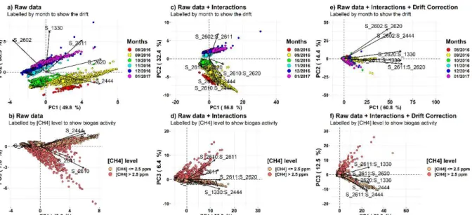
The PCA's results have been labelled considering the month (Fig. 3a, c and e) and methane concentration level (Fig. 3b, d and f). On the one hand, we observed that PC2 (38.9% of explained variance) was linked to the signal break noted in October 2016 in addition to a sensors drift denoting a monthly evolution of the baseline signal (Fig. 1 and 3a) while PC3 (7.6%) was partially linked to biogas activity over the MSW site (Fig. 3b). On the other hand, PC1(49.8%) appeared to be related to biogas composition, especially to ammonia and VOCs. MOS gas sensors which contributed mostly to PC1 were TGS2620 (with 27.14% as a percentage of contribution) and TGS2444 (26.03%). A statistical analysis of the individual's contributions to PC3 of records with methane concentration greater and less than 2.5 ppm showed that records with methane concentration greater than 2.5 ppm were the most contributors (p-value of Wilcoxon test < 2.2 ∙ 𝑒 ). The full information about biogas captured by PCA was well summarised by PC1 and PC3.

Fig. 3. PCA plots of three datasets. Original dataset (a, b), dataset with interactions (c, d) and dataset with drift correction and interactions (e, f). Months have been represented by rainbow colour and the biogas activity over the MSW presented by two classes (no activity: [CH4] <= 2.5 ppm; activity: [CH4] > 2.5 ppm). Arrows have represented variables with a significant contribution (raw sensors data and interactions) to PCA dimensions.

Considering the dataset with six-order interactions of MOS sensors (Fig. 3c and d), there was a change in the percentage of explained variances distribution compared with previous findings (56.8% for PC1, 32.4% to PC2 and 6.4% for PC3). More surprisingly, terms representing interactions between MOS gas sensors (2nd _{order interactions) were most contributors to PCA dimensions (e.g. S}

1330∙S2444 with 7.56% to PC1 and S2602∙S2611 with 8.89% to PC2). In Fig. 3e and f, there was clear evidence that the drift correction played its role. No signal break and drift effect have been noted as it was the case on Fig. 4a and b. On the other hand, Fig. 4f also showed a clear separation of the dataset by PC1 and PC3, considering the biogas activity level on MSW.

A possible explanation for the break, observed on signal (Fig. 1c and 2c) and PCA plots (Fig. 3a and c), might be a change in the chemical composition of the surrounding air mixture over the MSW occurred in October 2016. However, a note of caution is due here since we have no additional information to corroborate that. According to recent studies, the reasons for MOS sensors drift could be poisoning or ageing of sensors or a continuous change of environmental conditions [29]. However, a clear distinction between a long term drift linked to the sensing device and "time drift" linked to external factors should be made[30]. In this study, we did not investigate the leading cause of drift, but we suspected that the relative humidity might have played a role.

The most striking observation on the findings is that neither the first component nor the second component, are bound to methane concentration. This particular situation might not be observed in the context of laboratory calibration, where the most important source of variability is the gas concentration. Previous research on MOS sensors calibration in the laboratory for methane detection showed that the concentration was bound to PC1 [31] but, the continuous measurements approach had not been used. Overall, findings mentioned before draw our attention to the importance of paying attention to the link between principal components and target gas concentration.

3.2 Quantile regression models development

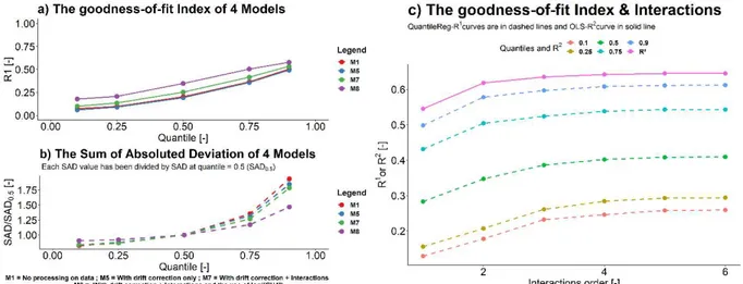
The QR model development’s results (Fig. 4a) showed that 𝑅 values were ranged from 0.072 to 0.577. The max value was observed when log transformation and interactions were used in the model configuration, irrespective of quantiles. Regardless of the model configuration, the highest value of 𝑅 was systematically observed for quantile 𝜏 = 0.9. It was apparent that the goodness-of-fit index increased with

conditional quantiles, showing a quite difference, between both tails (𝜏 = 0.1 and 0.9) and the median (𝜏 = 0.5). A possible explanation for the increase of 𝑅 might be the shape of methane concentration distribution (Fig. 2a).

Fig. 4. The goodness-of-fit index (a) and the sum of absolute Deviation (b) of 4 model configurations with respect to conditional quantiles tau = 0.1, 0.25, 0.5, 0.75 and 0.9. (c) The goodness-of-fit index (R and R ) evolution with interactions up to the sixth order.

In contrast to 𝑅 , SAD showed errors more important for quantile 𝜏 = 0.75, 𝜏 = 0.9 and for less complex model configurations (model without full data processing – see Fig. 4b). Consequently, we decided to use the model with 𝜏 = 0.5, sensors interactions and logarithm transform as the predictive model. Quantile regression models at 𝜏 = 0.1 and 𝜏 = 0.9, for their part, were used to check whether there were similar observations regarding coefficient terms.

Adding interactions as predictors to the model equation led to a more complex model and increased goodness-of-fit index. That increase can be explained by Equations 2 and 3. A complex model's objective function value (with several independent terms) will always be lowest than the one from a restricted model (a model with no independent terms). To select which interactions order should be used, we compared 𝑅 and 𝑅 considering interactions up the 6th _{order (Fig. 4c). We observed that 𝑅 was always higher than} 𝑅 _. , and after the 3rd _{order, there was no significant increase in 𝑅 . In the light of these results and given} the overfitting risk, the 2nd _{order has been preferred.}

3.3 Cross-validation and model selection

The cross-validation results are presented in Fig. 5a and 5b. In contrast to previous findings, the quantile regression model at 𝜏 = 0.5 showed a cross-validation curve with minimal error compared to the quantile regression model at 𝜏 = 0.1 (Fig. 4b). We also found that the 𝜆 values were close to 0. In that situation, many coefficients in the models were not set to zero preserving hence overfitting. Spencer et al. [32] gave the same remark about the use of 𝜆 and proposed using a new tuning parameter called 𝜆 . It is computed between 𝜆 and a 𝜆 value where the cross-validation error starts to increase significantly. We used the same approach (Fig. 5b) and for quantiles 𝜏 = 0.1, 0.5 and 0.9, we found respectively 0.006, 0.024 and 0.022 as 𝜆 values with 0.320, 0.248 and 0.538 as cross-validation errors respectively.

Fig. 5. (a) The Lasso Cross-validation curves of quantile regression models, and (b) the lambda midfel selection method.

The final equation for quantile 𝜏 = 0.5 obtained after model selection was:

log ([CH ]) . = 0.77 + 0.001 ∗ 𝑃𝐶 + (−0.001) ∗ 𝑃𝐶 + 0.11 ∗ 𝑃𝐶 + 0.03 ∗ 𝑃𝐶 + 0.26 ∗ 𝑃𝐶 + 0.1 ∗

𝑃𝐶 + 0.49 ∗ 𝑃𝐶 + (−0.07) ∗ 𝑃𝐶 + 0.22 ∗ 𝑃𝐶 + (−0.11) ∗ 𝑃𝐶 + (−0.34) ∗ 𝑃𝐶 + (−0.12) ∗ 𝑃𝐶 +

(−0.46) ∗ 𝑃𝐶 + 2.01 ∗ 𝑃𝐶

Fig. 6 has been made to help to understand this equation. It presents MOS gas sensors contributions (main effects and interactions), with predictors (PCA dimensions) associated with their respective slope parameters, percentage of explained variances, and correlations with [CH4].

At first sight, all PCA dimensions with negative coefficients were found negatively correlated with [CH4]. Excepted for PC7, PCA dimensions associated with null slope parameters had non-significant correlation with [CH4] (p-value < 0.05). Some of them showed contributions from MOS sensors non-sensitive to methane (e.g. PC5 with 3.47% of explained variance and with S2602 as the most important contributor) or contributions from interactions between non-sensitive sensors (e.g. PC10 with 0.22% of explained variance and S2602∙S2444 as the most important contributor).

Unsurprisingly, PC1 and PC2 slope parameters were found very low, despite the percentage of explained variance associated with them. We showed in section 3.1 that these dimensions were weakly linked to methane. More interesting, predictors with some high slope parameters, in absolute value, were those that had greater contributions from MOS sensors interactions (e.g. PC11 with 0.19% of explained variance and S2610∙S2444 and S2620∙S1330 as most important contributors). The same observation was made for both quantiles 𝜏 = 0.1 and 𝜏 = 0.9.

Although the final value of coefficient terms depended on 𝜆, there was no doubt that the cross-validated model described the relation between MOS sensors conductances and methane concentration.

Fig. 6. MOS gas sensors contributions (main effects and interactions) on PCA dimensions ordered following the absolute value of associated model coefficients. The percentage of explained variance on PCA dimensions is also given with their respective Pearson's correlation coefficients.

3.4 Quantile regression model predictions

This section showed the prediction results of the two cases described in section 2.8. Fig. 7 (case 2) showed for all models a poor agreement of predictions with exact values except for model with the best single sensor. The model with full processing being the one with the most important percentage error. In contrast, good MAPE and PLS values were obtained for the case 1 (Fig. 8), (30.95%, 38.78%, 39.79% and 51.97% as values with full processing and simple processing best single sensors and PLS, respectively). The model with the full processing correctly predicted peaks denoting biogas leakages.

Firstly, the results in figures 7 and 8 inform us that QR and PLS regression showed similar results. However, we cannot claim that one is better than the other since the QR predicts a median value and PLS based on least square approach predicts a mean value. The poor agreement found with testing data taken in September 2016 (case 2) could be explained by the signal level observed for some sensors. It was higher during this period than the remaining one (see Fig. 2c). This result is somewhat disappointing, but it gives a short overview of model sensitivity.

Fig. 7. (a) Quantile regression (QR) and PLS models predictions with testing data taken in September 2016. The dark blue and red lines represent the median regression prediction with full and simple processing, respectively; the orange band corresponds to the distance between the predicted concentration with tau = 0.1 and 0.9 quantiles. The magenta line and green lines are the PLS regression and QR with best single sensors (TGS2610). The black curve defines the exact log concentration of CH4. MAPE and root mean square percentage error (RMSPE) are given as model performance metrics. (b) The predicted value versus test value is proposed to compare models’ performances.

Fig. 8. Quantile regression (QR) and PLS models predictions with testing data taken in January 2017. The dark blue and red lines represent the median regression prediction with full and simple processing, respectively; the orange band corresponds to the distance between the predicted concentration with tau = 0.1 and 0.9 quantiles. The magenta line and green lines are the PLS regression and QR with best single sensors (TGS2610). The black curve defines the exact log concentration of CH4. MAPE and root mean square percentage error (RMSPE) are given as model performance metrics. (b) The predicted value versus test value is proposed to compare models’ performances.

Secondly, mixed results observed in Fig. 7 and 8 emphasise several matters of interest: How many sensors could be used (all sensors or the single one)? What kind of sensors (slightly higher sensitivity to combustible gases with respect to other compounds or not)? How important is the data processing method (full or simple )? How important is the training dataset (with all potential variability sources or not)? Furthermore, the purpose of using MOS sensors array in a portable device for field monitoring should be taken into account. Regarding QR performances with the best single sensor and the full processing, the full processing should be taken and redundant sensors removed in the sensor array. There is no need for two sensors showing

similar response to a given compound than the others. So, rather than using only one sensor, a sensor array with 3-4 MOS sensors that could be linked to external conditions encountered in the field (sensors with overlapping sensitivities) is the best choice.

Overall, we were satisfied with the results obtained with this methodology despite having a tricky dataset— moreover, these promising results with the quantile regression call for further investigations (for instance, a complete sensitivity analysis). It may help to (i) understand the impact of input variables (MOS sensors), (ii) explore the contribution broadly from each single data processing (drift correction, the addition of interactions and PCA for new features extraction) used before model training.

This paper did not intend to compare the PLS regression with QR, but to show how interesting could be the QR for gas monitoring with MOS sensors and open a possible area of research. Indeed, the quantile regression gives the possibility of investigating the output variable at many points of the conditional distribution, allowing to get a detailed analysis of regression [16,17]. As an example, not investigated in this paper, complete information about the relationship between MOS sensors' conductance and the dependent variable (methane concentration) at any quantile of the non-normal data distribution could be highlighted.

3.4 Conclusions

This paper aimed to develop and explore a field calibration model's forecast ability for CH4 estimation with a MOS gas sensors array. The methodology was based on a quantile regression approach and gas sensors interactions. Even if the used data were far from being perfect, we found that with appropriate pre-processing and setting up, the model gave an acceptable estimation (MAPE = 30.95 %) and can be used further for prediction over the same site. This study also showed the necessity to be cautious when using several pre-processing methods before training the model. It is also essential to consider temporal signal evolution for calibration development.

The current research was not explicitly designed to investigate which drift correction method could be the best one. Investigations based on the overview of the different drift correction methods given by Di and Falasconi [33] and Romain [30] could be an area of future research. Notwithstanding this limitation, this study showed that all of these methods (drift correction, the addition of interaction, feature extraction from PCA and quantile regression) brought a significant improvement. The same methods could be used to build a new model with new or other MOS gas sensors and used with a ground mobile robot or a drone. This study should be seen as a first trial and will be followed by complete experimentations in labs.

Quantile regression has been rarely used with MOS sensor array data. For field or laboratory application where data may be non-normal, this technique may be an efficient alternative to OLS. It is also the first time that a multiplicative combination of sensor signals has been considered. The results looked surprisingly powerful. Combining PCA (with different original variables and considering their interactions) seems to be a method that increases cross-sensitive sensor array performance. PCA on interactions sensors values + quantile regression had never been done before, and results promote this approach for future research. Credit Author Statement

Eric Martial TAGUEM: Conceptualisation, methodology, software, formal analysis, investigation, writing-original draft preparation, writing-review & editing, visualisation.

Luisa MENNICKEN: Conceptualisation, methodology, software, investigation, data curation, writing-original draft preparation, writing-review & editing, visualisation.

Anne-Claude ROMAIN: Conceptualisation, methodology, formal analysis, writing-review & editing, supervision, project administration.

This research was funded by the GRoNe Project from the INTERREG - Projets INTERREG V (2014-2020) – Grant ID : 024-4-09-076. We also thank ISSeP (Institut Scientifique de Service Public) for their instruments and data.

Declaration of Competing Interest:

The authors declare that they have no conflict of interest. References

[1] S. Yang, R. Talbot, M. Frish, L. Golston, N. Aubut, M. Zondlo, C. Gretencord, J. McSpiritt, Natural Gas Fugitive Leak Detection Using an Unmanned Aerial Vehicle: Measurement System Description and Mass Balance Approach, Atmosphere. 9 (2018) 383. https://doi.org/10.3390/atmos9100383. [2] European Commission. Joint Research Centre., JRC reference report on monitoring of emissions to

air and water from IED installations: industrial emissions directive 2010/75/EU (integrated pollution prevention and control)., Publications Office, LU, 2018. https://data.europa.eu/doi/10.2760/344197 (accessed November 23, 2020).

[3] A. Collier-Oxandale, J.G. Casey, R. Piedrahita, J. Ortega, H. Halliday, J. Johnston, M.P. Hannigan, Assessing a low-cost methane sensor quantification system for use in complex rural and urban environments, Atmospheric Meas. Tech. 11 (2018) 3569–3594. https://doi.org/10.5194/amt-11-3569-2018.

[4] M.I. Mead, O.A.M. Popoola, G.B. Stewart, P. Landshoff, M. Calleja, M. Hayes, J.J. Baldovi, M.W. McLeod, T.F. Hodgson, J. Dicks, A. Lewis, J. Cohen, R. Baron, J.R. Saffell, R.L. Jones, The use of electrochemical sensors for monitoring urban air quality in low-cost, high-density networks, Atmos. Environ. 70 (2013) 186–203. https://doi.org/10.1016/j.atmosenv.2012.11.060.

[5] J. Burgués, S. Marco, Low Power Operation of Temperature-Modulated Metal Oxide Semiconductor Gas Sensors, Sensors. 18 (2018) 339. https://doi.org/10.3390/s18020339. [6] M. van den Bossche, N.T. Rose, S.F.J. De Wekker, Potential of a low-cost gas sensor for

atmospheric methane monitoring, Sens. Actuators B Chem. 238 (2017) 501–509. https://doi.org/10.1016/j.snb.2016.07.092.

[7] N. Castell, F.R. Dauge, P. Schneider, M. Vogt, U. Lerner, B. Fishbain, D. Broday, A. Bartonova, Can commercial low-cost sensor platforms contribute to air quality monitoring and exposure estimates?, Environ. Int. 99 (2017) 293–302. https://doi.org/10.1016/j.envint.2016.12.007. [8] L. Spinelle, M. Gerboles, M.G. Villani, M. Aleixandre, F. Bonavitacola, Field calibration of a

cluster of low-cost commercially available sensors for air quality monitoring. Part B: NO, CO and CO2, Sens. Actuators B Chem. 238 (2017) 706–715. https://doi.org/10.1016/j.snb.2016.07.036. [9] J.M. Barcelo-Ordinas, M. Doudou, J. Garcia-Vidal, N. Badache, Self-calibration methods for

uncontrolled environments in sensor networks: A reference survey, Ad Hoc Netw. 88 (2019) 142– 159. https://doi.org/10.1016/j.adhoc.2019.01.008.

[10] Drift reduction for metal-oxide sensor arrays using canonical correlation regression and partial least squares, in: Electron. Noses Olfaction 2000, 0 ed., CRC Press, 2001: pp. 157–162.

https://doi.org/10.1201/9781482268904-29.

[11] J. Burgués, S. Marco, Multivariate estimation of the limit of detection by orthogonal partial least squares in temperature-modulated MOX sensors, Anal. Chim. Acta. 1019 (2018) 49–64.

https://doi.org/10.1016/j.aca.2018.03.005.

[12] S. De Vito, E. Massera, M. Piga, L. Martinotto, G. Di Francia, On field calibration of an electronic nose for benzene estimation in an urban pollution monitoring scenario, Sens. Actuators B Chem. 129 (2008) 750–757. https://doi.org/10.1016/j.snb.2007.09.060.

[13] N. Zimmerman, A.A. Presto, S.P.N. Kumar, J. Gu, A. Hauryliuk, E.S. Robinson, A.L. Robinson, R. Subramanian, A machine learning calibration model using random forests to improve sensor performance for lower-cost air quality monitoring, Atmospheric Meas. Tech. 11 (2018) 291–313. https://doi.org/10.5194/amt-11-291-2018.

[14] S. Marco, A. Gutierrez-Galvez, Signal and Data Processing for Machine Olfaction and Chemical Sensing: A Review, IEEE Sens. J. 12 (2012) 3189–3214.

https://doi.org/10.1109/JSEN.2012.2192920.

[15] R. Koenker, G. Bassett, Regression Quantiles, Econometrica. 46 (1978) 33. https://doi.org/10.2307/1913643.

[16] M. Furno, Goodness of Fit and Misspecification in Quantile Regressions, J. Educ. Behav. Stat. 36 (2011) 105–131. https://doi.org/10.3102/1076998610379134.

[17] M. Furno, Predictions in Quantile Regressions, Open J. Stat. 04 (2014) 504–517. https://doi.org/10.4236/ojs.2014.47048.

[18] J. Nicolas, A.-C. Romain, C. Ledent, The electronic nose as a warning device of the odour emergence in a compost hall, Sens. Actuators B Chem. 116 (2006) 95–99.

https://doi.org/10.1016/j.snb.2005.11.085.

[19] Anne-Claude Romain, Noemie Molitor, Gilles Adam, Emerance Bietlot, Catherine Collard, Comparison low cost chemical sensors analytical instruments for odour monitoring in municipal waste plants, Chem. Eng. Trans. 54 (2016) 211–216. https://doi.org/10.3303/CET1654036. [20] S.K. Chaulya, G.M. Prasad, Sensing and monitoring technologies for mines and hazardous areas:

monitoring and prediciton technologies, Elsevier, Amsterdam, 2016.

[21] K.H. Liland, T. Almøy, B.-H. Mevik, Optimal Choice of Baseline Correction for Multivariate Calibration of Spectra, Appl. Spectrosc. 64 (2010) 1007–1016.

https://doi.org/10.1366/000370210792434350.

[22] R. Koenker, J.A.F. Machado, Goodness of Fit and Related Inference Processes for Quantile Regression, J. Am. Stat. Assoc. 94 (1999) 1296–1310.

https://doi.org/10.1080/01621459.1999.10473882.

[23] M. Buchinsky, Recent Advances in Quantile Regression Models: A Practical Guideline for Empirical Research, J. Hum. Resour. 33 (1998) 88. https://doi.org/10.2307/146316. [24] B.L. Cook, W.G. Manning, Thinking beyond the mean: a practical guide for using quantile

regression methods for health services research, (2013) 5.

[25] H. Zou, M. Yuan, Regularised simultaneous model selection in multiple quantiles regression, Comput. Stat. Data Anal. 52 (2008) 5296–5304. https://doi.org/10.1016/j.csda.2008.05.013. [26] Y. Wu, Y. Liu, VARIABLE SELECTION IN QUANTILE REGRESSION, Stat. Sin. 19 (2009)

801–817.

[27] S. Kucheryavskiy, mdatools – R package for chemometrics, Chemom. Intell. Lab. Syst. 198 (2020) 103937. https://doi.org/10.1016/j.chemolab.2020.103937.

[28] C.M. Andersen, R. Bro, Variable selection in regression-a tutorial, J. Chemom. 24 (2010) 728–737. https://doi.org/10.1002/cem.1360.

[29] M. Holmberg, F.A.M. Davide, C. Di Natale, A. D’Amico, F. Winquist, I. Lundström, Drift counteraction in odour recognition applications: lifelong calibration method, Sens. Actuators B Chem. 42 (1997) 185–194. https://doi.org/10.1016/S0925-4005(97)80335-8.

[30] A.C. Romain, J. Nicolas, Long term stability of metal oxide-based gas sensors for e-nose environmental applications: An overview, Sens. Actuators B Chem. 146 (2010) 502–506. https://doi.org/10.1016/j.snb.2009.12.027.

[31] E.M. Taguem, A.-C. Romain, MOS sensors array for methane monitoring with UAS, in: 2019 IEEE Int. Symp. Olfaction Electron. Nose ISOEN, IEEE, Fukuoka, Japan, 2019: pp. 1–4.

https://doi.org/10.1109/ISOEN.2019.8823371.

[32] B. Spencer, O. Alfandi, F. Al-Obeidat, A Refinement of Lasso Regression Applied to Temperature Forecasting, Procedia Comput. Sci. 130 (2018) 728–735.

https://doi.org/10.1016/j.procs.2018.04.127.

[33] S. Di, M. Falasconi, Drift Correction Methods for Gas Chemical Sensors in Artificial Olfaction Systems: Techniques and Challenges, in: W. Wang (Ed.), Adv. Chem. Sens., InTech, 2012. https://doi.org/10.5772/33411.