A brain-computer interface for navigation in virtual reality

A Brain-Computer Interface for

navigation in virtual reality

Bilal Alchalabi

Institut de Génie Biomédical

Université de Montréal

MÉMOIRE PRÉSENTÉ EN VUE DE L’OBTENTION

DU DIPLÔME DE MAÎTRISE ÈS SCIENCES APPLIQUÉES

(GÉNIE BIOMÉDICAL)

Janvie 2013

Université de Montréal

Institut de Génie Biomédical

Ce mémoire intitulé:

"A Brain-Computer Interface for

navigation in virtual reality"

Présenté par:

Bilal Alchalabi

a été évalué par un jury composé des personnes

suivantes:

Pr. Pierre Savard, président-rapporteur

Pr. Jocelyn Faubert, directeur de recherche

Résumé :

L'interface cerveau-ordinateur (ICO) décode les signaux électriques du cerveau requise par l’électroencéphalographie et transforme ces signaux en commande pour contrôler un appareil ou un logiciel. Un nombre limité de tâches mentales ont été détectés et classifier par différents groupes de recherche. D’autres types de

contrôle, par exemple l’exécution d'un mouvement du pied, réel ou imaginaire, peut modifier les ondes cérébrales du cortex moteur. Nous avons utilisé un ICO pour déterminer si nous pouvions faire une classification entre la navigation de type marche avant et arrière, en temps réel et en temps différé, en utilisant différentes méthodes. Dix personnes en bonne santé ont participé à l’expérience sur les ICO dans un tunnel virtuel. L’expérience fut a était divisé en deux séances (48 min chaque). Chaque séance comprenait 320 essais. On a demandé au sujets d’imaginer un déplacement avant ou arrière dans le tunnel virtuel de façon aléatoire d’après une commande écrite sur l'écran. Les essais ont été menés avec feedback. Trois

électrodes ont été montées sur le scalp, vis-à-vis du cortex moteur. Durant la 1re

séance, la classification des deux taches (navigation avant et arrière) a été réalisée par les méthodes de puissance de bande, de représentation temporel-fréquence, des modèles autorégressifs et des rapports d’asymétrie du rythme β avec

classificateurs d’analyse discriminante linéaire et SVM. Les seuils ont été calculés en temps différé pour former des signaux de contrôle qui ont été utilisés en temps réel

durant la 2e séance afin d’initier, par les ondes cérébrales de l'utilisateur, le

déplacement du tunnel virtuel dans le sens demandé. Après 96 min d'entrainement, la méthode « online biofeedback » de la puissance de bande a atteint une précision de classification moyenne de 76 %, et la classification en temps différé avec les rapports d’asymétrie et puissance de bande, a atteint une précision de classification d’environ 80 %.

.

Mots-clés: Interface cerveau-ordinateur(ICO), synchronisation lié à l'événement, Moteur imaginaire, électroencéphalogramme (EEG), Réalité Virtuelle, Navigation, classification de EEG.

Abstract:

A Brain-Computer Interface (BCI) decodes the brain signals representing a desire to do something, and transforms those signals into a control command. However, only a limited number of mental tasks have been previously detected and classified. Performing a real or imaginary navigation movement can similarly change the brainwaves over the motor cortex. We used an ERS-BCI to see if we can classify between movements in forward and backward direction offline and then online using different methods. Ten healthy people participated in BCI experiments comprised two-sessions (48 min each) in a virtual environment tunnel. Each session consisted of 320 trials where subjects were asked to imagine themselves moving in the tunnel in a forward or backward motion after a randomly presented (forward versus backward) command on the screen. Three EEG electrodes were mounted bilaterally on the scalp over the motor cortex. Trials were conducted with feedback. In session 1, Band Power method, Time-frequency representation, Autoregressive models and asymmetry ratio were used in the β rhythm range with a Linear-Discriminant-analysis classifier and a Support Vector Machine classifier to discriminate between the two mental tasks. Thresholds for both tasks were computed offline and then used to form control signals that were used online in session 2 to trigger the virtual tunnel to move in the direction requested by the user's brain signals. After 96 min of training, the online band-power biofeedback training achieved an average classification precision of 76 %, whereas the offline classification with asymmetrical ratio and band-power achieved an average classification precision of 80%.

Keywords: Brain-Computer Interface, Event-Related Synchronization, Motor Imagery, electroencephalogram(EEG), Virtual Reality, Navigation, EEG classification

Table of Contents:

Résumé……….…..….…..iii

Abstract ...iv

Table of Contents ...v

List of Figures ...viii

List of Tables...x

List of Abbreviation...xi

Remérciments...xii

Chapter 1 Introduction

1.2. Hypothesis and originality...4

1.3. Objectives...4

1.3.1. General Objective...4

1.3.2. Specific Objectives...4

1.4. Thesis Outline...5

Chapter 2 Electroencephalography (EEG)

2.2. Brain anatomy and function...8

2.3. Neurons and brainwaves...11

2.4. EEG recordings and techniques...12

2.4.1. Electrodes & electrode placement...14

2.4.2. Mono-polar and bipolar recordings...16

2.5. EEG signals used to drive BCIs...17

Chapter 3 Brain Computer Interfaces (BCIs)

3.2. BCI design approaches: Patter recognition Vs Operant conditioning...20

3.3. BCI control approaches: synchronous Vs asynchronous...20

3.4. BCI framework...21

Chapter 4 BCI signal processing

4.1.1. Temporal filters...24

4.1.2. Spatial filters...24

4.1.3. Independent Component Analysis (ICA)...25

4.1.4. Common Spatial Patterns (CSP)...25

4.2. Feature extraction...26

4.2.1. Temporal Methods...26

4.2.1.1. Signal amplitude...26

4.2.1.2. Band power features...26

4.2.1.3. Autoregressive parameters...28

4.2.2. Time-frequency representations with Short-time Fourier transform...31

4.2.3.1. Power spectral density features...32

4.2.1.2. Power Asymmetry Ratio features...33

4.3. Feature selection and dimensionality reduction………34

4.4. Feature Classification Methods...34

4.4.1. Linear Discriminant Analysis (LDA)...34

4.4.2. Support Vector Machines...35

4.4.3. Multilayer Neural Networks...36

Chapter 5 BCI applications

5.2. P300 Speller and Character Recognition...37

5.3. ERS/ERD Cursor Control...39

5.4. A Multi-command Steady State Visual Evoked Potential BCI...43

5.5. FES control by thoughts...44

Chapter 6 BCI-based Virtual reality applications

6.2. Walking through a Virtual City by Thought...46

6.3. Self-paced exploration of the Austrian National Library through thought...47

6.4. Virtual Smart Home Controlled By Thoughts...48

6.5. Controlling an avatar to explore a virtual apartment using an SSVEP-BCI...49

6.6. BCI-based VR applications for disabled subjects...49

Chapter 7 Experiment

7.2. Overall system flowchart...52

7.3. Equipment...53

7.3.1. Computer Specification...53

7.3.2. Wireless EEG Equipment...53

7.3.3. Virtual Reality Equipment...54

7.3.4. Virtual Reality Tunnel...55

7.3.5. Biograph Software...57

7.3.5. MATLAB...58

7.4. Methodology...58

7.5. Signal Pre-Processing...66

7.6. Feature extraction and selection...67

7.6.1. Time-Frequency Representation Spectrograms...67

7.6.2. Band Power and ERD/ERS calculation………...68

7.6.3. Power Spectral Density Asymmetrical Ratio...69

7.6.4. Auto-regression models...69

7.7. Classification………..70

7.8. Results and discussions...72

7.8.1. Online TFR………..………....72

7.8.2. Online Band-power ERD/ERS Biofeedback……….………..…73

7.8.3. Offline analysis, feature selection and classification……….…………..……....79

Chapter 8 Conclusions & future work

8.1. ERS-BCI...85

8.2. Future of BCI technology...88

References...90

Appendix A: XML code………...97

Appendix B: Flex-comp infinity technical specifications...98

List of figures:

Figure 2-1: Human brain Lobes………..………..……….8

Figure 2-2: Human Brain functions………..………9

Figure 2-3: the Neuron………..………11

Figure 2-4: EEG electrodes and sensor……….……….14

Figure 2-5: Needle electrodes……….………….14

Figure 2-6: Electrodes Cap………..14

Figure 2-7(a): 10-20 International System………15

Figure 2-7(b): Selection of 10–10 electrode positions in a realistic display. Lateral, frontal and posterior views. The head and brain contours based on typical models. Black circles indicate positions of the original 10–20 system, grey circles indicate additional positions in the 10–10 extension[79]……….16

Figure 3-1: BCI framework………..21

Figure 4-1: ERD calculation Method……….27

Figure 4-2: AR model………..28

Figure 4-3: ARX model………..28

Figure 4-4: TFR spectrogram at channels C3 and C4 with motor imagery of right hand movement [12]……….………..31

Figure 4-5: classification basics……….………..35

Figure 4-6: Multi-Perceptron Neuron Network………36

Figure 5-2(a): P300 Speller Paradigm………..37

Figure 5-2(b): P300 wave……….37

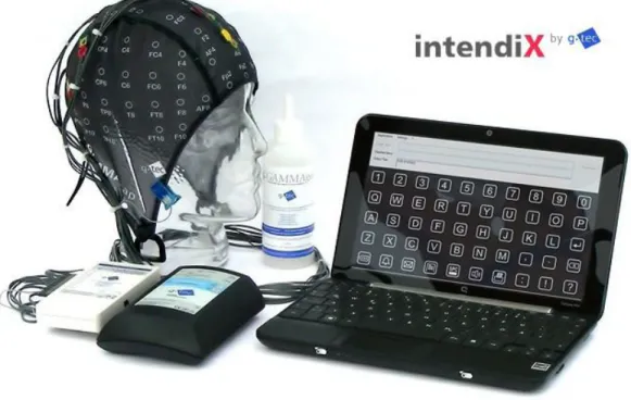
Figure 5-2 (c): Setup of EEG operated spelling device and a skull cap, Source: www.intendix.com...38

Figure 5-3: ERD-BCI paradigm………..42

Figure 5-4: Multi-Command SSVEP-BCI……….43

Figure 5-5: FES controlled by thoughts………..44

Figure 6-1: The application “use the force "……….………..……….45

Figure 6-2: Walking through a virtual city by thoughts………..46

Figure 6-3: Exploration of the national Austrian Library through Thoughts………...47

Figure 6-4: Virtual Smart Home Controlled By Thoughts……….……….48

Figure 6-5: Virtual Smart Home Controlled By Thoughts………..49

Figure 6-6: Controlling an avatar to explore a virtual apartment using an SSVEP-BCI………….49

Figure 6-7: BCI-based VR applications for disabled subjects………..51

Figure 7-1: Overall system Flowchart………..53

Figure 7-2: The Flex Comp Infiniti™ encoder……….54

Figure 7-3: ICUBE………55

Figure 7-4: Virtual Reality Tunnel………..55

Figure 7-5: Peripheral visual field condition………56

Figure 7-6: Channel Editor installed with Biograph………57

Figure 7-7: localizing EEG electrodes placements on the scalp……….59

Figure 7-8: localizing Cz electrode placement on the scalp……….60

Figure 7-9: localizing C3,C4 electrode placement on the scalp……….60

Figure 7-11: Attaching EEG electrode to the scalp……….61

Figure 7-12: Attaching reference electrodes to the ear lobe……….61

Figure 7-13: A subject in the tunnel……….61

Figure 7-14: One trial Paradigm of the BCI in our research……….62

Figure 7-15: Online TFR over C3 and C4……….72

Figure 7-16: β-ERS at channels C4 and C3 respectively, and at the frequency band 25-30 Hz for subject 7………..73

Figure 7-17: Beta-ERS (over C3 and C4) method accuracy results for subject3………...76

Figure 7-18: Run 4 average accuracy for all subjects………77

Figure 7-19: Beta-ERS method accuracy across all subjects………78

Figure 7-20: Classification of power spectral density asymmetrical ratio between C3-C4 within the β band varied with epochs and averaged across 10 subjects………80

Figure 7-21 state-space model order selection for β-PSD As.R on the left and β-BP on the right………81

Figure 7-22: Classification accuracy over β-ERS for the online Biofeedback using 2 EEG channels (session 2), the Power Spectral Density Asymmetrical ratio with LDA classifier using 2 EEG channels (session 1) and the Band-Power modeled with ARburg when classified with SVM using 3 EEG channels (session 1)………84

List of tables:

Table 2-1: Cortical areas Functions[79]……….…….….10

Table 2-2: EEG frequency bands[79],[43],[89],[75],[35],[24]..………....…12

Table 2-3: EEG signals to drive BCIs[5],[35]……….………..…...16

Table 7-1: Methodology and protocol………..………...…….54

Table 7.2 results of the ERS Biofeedback for subject 3………..75

Table 7.3 the results of the online beta-ERS biofeedback across all subjects……….77

Table 7.4 PSD classification with SVM when varying C factor………...81

Table 7.5 Classification results for PSD asymmetrical ratio over beta band varying with model order and averaged across 10 subjects……….…82

Table 7.6 comparisons between session 1 offline classification over beta band and the session 2 online biofeedback for all subjects……….82

Table 7.7 classification of beta band-power from 3 EEG channels varied with model order for subject 3………..83

Table 7.8 session 2 classification results for PSD asymmetrical ratio between C3-C4 classified with LDA, Band-Power from C3-C4-CZ modeled with ARburg and classified with SVM, and Band-Power online biofeedback for all subjects……….84

List of Abbreviations:

AAR Adaptive Auto-Regression

AR Auto-Regression

ARMA Auto-Regression with Moving Average

ARMAX Auto-Regression with Moving Average & exogenous output

As.R Asymmetrical Ratio

ARX Auto-Regression with exogenous input

BCI Brain-Computer Interface

BP Band-Power

CAR Common Average Reference

CRBF Cerebral Blood Flow

CSP Common Spatial Pattern

ECG Electrocardiogram

EEG Electroencephalogram

EMG Electromyogram

EOG Electrooculogram

ERD Event Related De-synchronization

ERS Event Related Synchronization

ERP Event Related Potential

FES Functional Electrical Stimulation

Fs Sampling Frequency

GA Genetic Algorithm

ICA Independent Component Analysis

IIR Infinite Impulse Response

LDA Linear Discriminant Analysis

LMS Least Mean Square

MPNN Multi Perceptron Neural Network

MRP Movement Related Potential

OC Operant Conditioning

PCA Principle Component Analysis

PR Pattern Recognition

PET Positron Emission Tomography

PSD Power Spectral Density

SCP Slow Cortical Potential

SSAEP Steady State Auditory Evoked Potential

SSVEP Steady State Visual Evoked Potential

STDEV Standard Deviation

STFT Short Time Fourier Transform

SVM Support Vector Machine

TFR Time-Frequency Representation

TH Threshold

VE Virtual Environment

VEP Visual Evoked Potential

Remerciments :

Tout d’abord je tiens à remercier une personne spéciale qui m'a soutenu pendant deux ans pour préparer ce mémoire. Prof. Jocelyn Faubert, tu étais un directeur unique avec un magnifique sens de l’humour, qui m'a donné de son précieux temps et m’a motivé à atteindre mes objectifs, merci beaucoup professeur de m'avoir accepté et de m’avoir permis de faire ce projet, merci pour la bourse que tu m’as offerte. J’ai beaucoup appris de toi. Merci beaucoup Isabelle Legault, l'assistante de mon directeur, pour m’avoir aidé plusieurs fois, merci pour tous tes conseils et précieux efforts. Merci beaucoup à mes collègues Rémy Allard et Vadim Sutyushev, qui m’ont aidé dans la programmation.

Merci à mon collègue Frederick Poirier pour tes précieux conseils. Merci à toute l’équipe du laboratoire de Psychophysiques et perception visuelle, pour votre soutien, vos encouragements et pour l’ambiance d’amitié que j’ai trouvé au labo. J’ai

vraiment eu beaucoup de plaisir à travailler avec vous.

Je tiens aussi à remercier les différents membres de mon jury d’avoir accepté de juger mon travail et mon mémoire.

Merci mes chers parents, Dr.Abdul Ghani Alchalabi et Dr. Khloud Sarraj, mes précieux cadeaux de dieu. Sans vous, sans votre soutien moral et financier, sans votre encouragement et sagesse, je ne serais pas devenu ce que je suis, je n'aurais pas été ici, et ce mémoire n'aurait jamais été écrit. Depuis l'enfance, vous m’avez toujours inspiré dans la recherche pour le savoir et la science. Je voulais vous rendre fières de moi.

Merci à mes frères et ma sœur, Dr.Omar Alchalabi, Besher Alchalabi et Dr.Maya Alchalabi, les fleurs de la famille, merci pour toutes les belles soirées et pour votre encouragement. Merci pour les succès Maya.

Des mercis très spéciaux à ma nouvelle famille, tant Aeda, oncle Issam, mes nouveaux frère et sœur Dr.Ahmad et Dr.Ola, merci de m’avoir accepté parmi vous et pour m'avoir offert cette très belle ambiance, honneur et le sentiment merveilleux de faire partie de votre famille. Avoir une famille come vous est une bénédiction.

Merci à mon premier directeur de thèse à l'université de Damas, Dr.Basel Douagi, qui m’a accepté au projet de l'année pré-finale du bac. Je ne t'oublierai jamais. Mon ami Saria Mohammed, tu as été un vrai ami et frère, j'ai eu beaucoup de plaisir à te rencontrer et à passer les weekends avec toi. Merci pour ton encouragement, pour être mon ami et pour le joli poème tu m’as écrit à mon anniversaire. Quand ce mémoire a été écrit, tu étais un bébé qui était en train de grandir doucement dans le ventre de sa mère, j'ai tellement pensé à toi. Merci mon fils Aboudeh pour venir et remplir notre vie de joie, et me donner le privilège de devenir ton papa.

Les derniers sont les premiers……Un merci spécial, un très gros merci à ma jolie femme adorable, mon amour et inspiration, Dr.Abir, je suis le plus heureux des hommes quand je suis avec toi, merci de m'aimer comme je suis, pour partager avec moi les plus beaux sentiments, merci pour chaque jour et chaque moment, merci pour ton encouragement et soutien pendant ces deux années, et merci pour la fabuleuse cuisine, tu es une femme merveilleuse.

Chapter 1

Introduction

1.1. Background

Can computers really read our minds? Can we ever truly forget our past? Can we control anything in the real world with only our thoughts? Brain-computer interaction has been a hot research concept since the beginning of the computer era. Since the first experiments of Electroencephalography (EEG), i.e. Brain waves recording on humans by Hans Berger in 1929, the idea that brain activity could be used as a communication channel has rapidly gained popularity [24].

However, it is only in 1964 that the first prototype of a Brain-Computer Interface (BCI) came out, in the laboratory of Dr.Grey Walter when he connected the EEG system of a patient to a slide projector so that the slide projector advanced whenever the patient’s brain activity indicated that he wanted to do so [8].

A BCI is a communication system that bypasses the body’s neuromuscular pathways, measures brain activity associated with the user’s intent and translates it into corresponding control signals to an electronic device, only by means of voluntary variations of his brain activity. Such a system appears as a particularly promising communication channel for persons suffering from severe paralysis, like those with the “locked-in” syndrome and, as such, is locked into their own body without any residual muscle control [24]. Therefore, a BCI appears as their only way of

communication, where their speech brain activity has been translated to a computer speller [100], [24], as well as their intention of moving their wheelchairs has been translated into real movements of those wheelchairs [24].

Studies to date show that humans can learn to use electroencephalographic activity (EEG) to control the movements of a cursor or other device in one or two

dimensions[27],[52],[96],[101],[30]. Both actual movement and activity movement imagery are accompanied by changes in the amplitudes of certain EEG rhythms, specifically 8–12 Hz mu rhythms and 18–30 Hz beta rhythms [35]. These changes are focused over sensorimotor cortex in a manner consistent with the homuncular organization of this cortical region [24].

It was also found that while observing movements performed by others, the observers’ cortical motor areas and spinal circuits were activated, reflecting the specific temporal and muscular pattern of the actual movement [10]. The BCIs of Wolpaw’s group in Albany and the Graz group are both based on motor imagery and classification of sensorimotor EEG rhythms , where they discovered that motor imagery (imagining a movement) can modify the neuronal activity in the primary sensory-motor areas in a very similar way as observable with a real executed movement [18],[59].

In the 1980s, Wolpaw et al. started on EEG-based cursor control in normal adults using band power centered at 9 Hz. They used an Auto-regressive model to compute power in a specific frequency band, where the sum power was used in a linear function to control the cursor's direction of movement [24]. However, and for the same goal, Yuanqing Li et al. in 2010 have controlled a 2-D cursor using a hybrid BCI, where they used both beta rhythm and P300 signals [101](The P300 is the positive component of the evoked potential that may develop about 300 ms after an item is flashed [5]).

Nowadays, the world of BCI is expanding very rapidly. One new field involves BCIs to control virtual reality (VR), including BCIs for games [37],[51],[84],[23],[29]. Virtual environments (VE) can provide an excellent testing ground for procedures that could be adapted to real world scenarios, especially for patients with disabilities. If people can learn to control their movements or perform specific tasks in a VE, this could justify the much greater expense of building physical devices such as a wheelchair or robot arm that is controlled by a BCI. One of the main goals of implementing BCI in VR is to understand how humans process dynamic visual scenes and how well they can interact with these natural environments. A better understanding of the normal brain will help us decipher the important mechanisms for certain activities such as way finding and reaching gestures that are critical in real life situations. Such basic understanding will also lead to a better understand of how neurodegenerative disorders such as how Alzheimer can influence daily living activities and help us find the right interventions to alleviate the impact of such disorders on quality of life of the patients.

The first efforts to combine VR and BCI technologies were In year 2000 and 2003 by Bayliss and Ballard who introduced a VR smart home in which users could control different things using a P300 BCI [6],[7].

Then in 2003, researchers showed that immersive feedback based on a computer game can help people learn to control a BCI based on imaginary movement more quickly than mundane feedback [42]. In year 2010, researchers used a steady-state visual evoked potential (SSVEP)-based BCI to navigate an avatar in virtual reality to two waypoints along a given path in two runs, by alternately focusing attention on one of three visual stimuli that were flickering at 12, 15 and 20 Hz [40]. Successful classifications of the following classes triggered the associated commands: turn 45° left, turn 45° right and walk one step ahead (Steady-state evoked potentials occur when sensory stimuli are delivered in frequencies high enough that the relevant neuronal structures do not return to their resting states). In [41] the same technique was used to control a character in an immersive 3-D gaming environment

In 2005 researchers in [54] used BCI for walking in a virtual street, in 2007 to visit and navigate in a virtual reality representation of the Austrian National library [76], and exploring a smart virtual apartment using a motor imagery-based BCI in 2009. In [53] Researchers used the BCI to navigate in virtual reality with only beta waves, where a 35 year old tetraplegic male subject learned to control a BCI, where the mid-central focused beta oscillations with a dominant frequency of approximately 17 Hz allowed the BCI to control VE . Only one single EEG channel was recorded bipolarly at Cz (foot representation area). One single logarithmic band power feature was estimated from the ongoing EEG. A simple threshold (TH) was used to distinguish between foot movement imagination (IC) and rest (INC). This study, which was based only on beta waves, has classified two different mental states: one directional

movement (forward) and a rest state but not for backward movement.

Brosseau-Lachine et al in [11] and [12] psychophysically studied Infants and made electrophysiological recordings of brain cells in cats’ response to radial optic flow fields, and found superior sensitivity for expansion versus contraction direction of motion in both studies. This is further supported by an imaging study with adults where the researchers have found a bias for expanding motion stimuli [77]. This dissociation may suggest that sensitivity to direction corresponding with forward

locomotion (expansion) develops at a faster rate than the opposite direction encountered when moving backwards (contraction).

Researchers in [77] found with PET scan that several loci of activation were observed for contraction and expansion condition in the same areas of the human brain, but the increase in rCBF in contraction was much lower than in the expansion condition in the right brain. So, we wanted to see in the present study if we could classify those two-directional movements in virtual reality from only 1, 2 or 3 EEG channels. Therefore, the main goal of the present project was to enhance navigation in virtual reality with the brainwaves by using beta ERS obtained from a small number of channels. Further, we wanted to see if we could classify two-directional movements (forward or backwards) in virtual reality from these channels so in the future a subject could efficiently navigate by altering the brain waves, freeing the limbs for other activities.

1.2. Hypothesis and originality

1) It is possible to distinguish and predict single-trial forward and backward movement commands with the methods proposed.

2) Backward commands will require more signal-training to achieve the same strength.

3) Motor imagery of forward-backward movement can activate the motor cortex similarly to real optic flow.

1.3. Objectives

1.3.1. General objective

The aim of the research is to navigate backward and forward in a virtual reality tunnel using biofeedback from the brainwaves.

1.3.2. Specific objectives

1. Design and investigate a short-training motor imagery BCI for navigation in virtual reality with:

 3 EEG channels (the later investigation and analysis would reveal if we can rely on 1 or 2 electrodes to use in the BCI).

2. Session1: Acquire EEG during an optic flow moving both forward and backward within a tunnel, and during imaging navigation in the virtual reality

 Use features extracted with different feature extraction methods and classification methods using MATLAB on session 1 data

3. Session 2: perform a short band-power training for navigation direction in the tunnel with Biograph (the EEG acquisition and biofeedback software)

 Perform offline classification of session 2 data in MATLAB using the session 1 data as training data

4. Compare MATLAB and Biograph efficiencies

After EEG acquisition, pre-processing and processing methods (IIR filtering ,Time-Frequency Representation and Band Power feature extractions) will be conducted via Biograph, then we want to import EEG data to MATLAB, where we will apply signal processing methods ( Auto-regression analysis , Band-Power, and power spectral density asymmetrical ratio), and then feed all these features to LDA classifier (Linear Discriminant Analysis) and SVM (Support Vector Machine) in order to classify these signals in an attempt to identify both movements; where we can later threshold the signals to control navigation direction in virtual reality.

1.4. Thesis Outline

Chapter 2 of this thesis will go through the main principals and methods of recording brain waves, as well as locations of recordings on the scalp in relation with the brain anatomy and physiological functions. Chapter 3 will introduce Brain computer Interfaces (BCI) and explain the fundamental approaches of BCI design and control, then the fourth chapter will go through some of the main signal processing

techniques used in pre-processing, feature extraction and selection, and

classification of signals [5], where these techniques are implemented in some BCI applications illustrated in the fifth chapter of the thesis, followed by chapter 6 which presents some BCI applications in Virtual Reality. Finally, chapter 7 presents the

experiments conducted for this research as well as the results, where the discussions and conclusion will be presented in chapter 8 of the thesis.

Chapter 2

Electroencephalography (EEG)

2.1. History

Richard Caton, In 1887, had recorded the first brain very-low-Amplitude electrical activity from the cerebral cortex of an experimental animal. In 1924 in Austria, the first human EEG recordings using metal strips pasted to the scalps of the subjects as electrodes were carried out by Hans Berger. He used a sensitive galvanometer as the recording instrument to record the μV brain signals, and was able to study the different waves of this electrical activity, which he gave the name

“electroencephalogram"[43].

Berger also reported that these brain waves were sort of periodic. He compared the slow brain waves during sleep to the brain waves during a mental activity or during a walk, and suggested, quite correctly, that EEG changed in a consistent and

recognizable fashion when the general status and health conditions of the subject changed. However, despite the insights provided by these studies, Berger’s original paper, published in 1929, did not generate much attention. It was not until 1934 that Adrian and Matthews confirmed Berger’s discoveries. They studied the “alpha rhythm”, 8-12 Hz from the occipital lobe and discovered that this rhythm

disappeared when a subject displayed any type of attention or alertness or focused on objects in the visual field. Moruzzi and Magoun in 1949, demonstrated the existence of pathways widely distributed through the central reticular core of the brainstem that were capable of exerting a diffuse activating influence on the cerebral cortex. This “reticular activating system” has been called the brain’s

response selector because it alerts the cortex to focus on certain pieces of incoming information while ignoring others. It is for this reason that a sleeping mother will immediately be awakened by her crying baby or the smell of smoke and yet ignores the traffic outside her window or the television playing in the next room [43].

2.2. Brain anatomy and function

The average adult human brain weighs around 1.4 kg. The brain is surrounded by cerebrospinal fluid that suspends it within the skull and protects it by acting as a motion dampener [79]. In relation to the stages of brain development, Carlson categorizes its components into three groups; the Forebrain, Midbrain and Hindbrain. Anatomically the brain can be divided into the three largest structures: The brain stem (hindbrain), the cerebrum and the cerebellum (forebrain). The functions of these structures are summarized as follows[79]:

• The brainstem controls the reflexes and autonomic nerve functions (respiration, heart rate, blood pressure).

• The cerebrum consists of the cortex, large fiber tracts (corpus callosum) and some deeper structures (basal ganglia, amygdala, hippocampus). It integrates information from all of the sense organs, initiates motor functions, controls emotions and holds memory and higher thought processes.

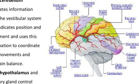
• The cerebellum integrates information from the vestibular system that indicates position and movement and uses this information to coordinate limb movements and maintain balance. • The hypothalamus and pituitary gland control visceral functions, body

temperature and behavioral responses such as feeding, drinking, sexual response, aggression and pleasure.

• The thalamus or specifically the thalamic sensory nuclei input is crucial to the generation and modulation of rhythmic cortical activity.

The cerebrum can be spatially sub-divided. Firstly into two hemispheres, left and right, connected to each other via the corpus callosum. The right one senses

Figure 2-1: Human Brain Parts

information from the left side of the body and controls movement on the left side. Similarly the left hemisphere is connected to the right side of the body. Each hemisphere can be divided into four lobes. They are [79]:

1. Frontal Lobes -involved with decision-making, problem solving, and planning

2. Occipital Lobes-involved with vision and color recognition

3. Parietal Lobes - receives and processes sensory information

4. Temporal Lobes - involved with emotional responses, memory, and speech

The cerebral cortex is the most relevant structure in relation to EEG measurement. It is responsible for higher order cognitive tasks such as problem solving, language comprehension and processing of complex visual information. Due to its surface position, the electrical activity of the cerebral cortex has the greatest influence on EEG recordings [79].

The functional activity of the brain is highly localized. This facilitates the cerebral cortex to be divided into several areas responsible for different brain functions.

Table 2-1: main cortical areas functions [79]

Cortex area

Function

Auditory complex processing of auditory information, detection of sound, Speech production and articulation

Prefrontal Problem solving, emotion, complex thought

Pre-motor Planning and Coordination of complex movement

Motor Initiation of voluntary movement

somatosensory Receives tactile information from the body

Gustatory area Processing of taste information

Wernicke’s Language comprehension

Visual Complex processing of visual information

Since the architecture of the brain is non-uniform and the cortex is functionally organized, the EEG can vary depending on the location of the recording electrodes. Most of the cortical cells are arranged in the form of columns, in which the neurons are distributed with the main axes of the dendrite trees parallel to each other and perpendicular to the cortical surface. This radial orientation is an important condition for the appearance of powerful dipoles.

It can be observed that the cortex, and within any given column, consist of different layers. These layers are places of specialized cell structures and within places of different functions and different behaviors in electrical response. An area of very high activity is, for example, layer IV, which neurons function to distribute information locally to neurons located in the more superficial (or deeper) layers. Neurons in the superficial layers receive information from other regions of the cortex. Neurons in layers II, III, V, and VI serve to output the information from the cortex to deeper structures of the brain. The anatomy of the brain is complex due its intricate structure and function. This amazing organ acts as a control center by receiving, interpreting, and directing sensory information throughout the body [43].

2.3. Neurons and brainwaves

The brain's electrical charge is

maintained by 1014 pyramidal neurons

and 1020 synapses. Neurons are

electrically charged (or "polarized") by membrane transport proteins that pump ions across their membranes. Neurons are constantly exchanging ions with the extracellular milieu, for example to

maintain resting potential and to propagate action potentials. Ions of similar charge repel each other, and when many ions are pushed out of many neurons at the same time, they can push their neighbours, who push their neighbours, and so on, in a wave. This process is known as volume conduction. When the wave of ions reaches the electrodes on the scalp, they can push or pull electrons on the metal on the electrodes. Since metal conducts the push and pull of electrons easily, the difference in push or pull voltages between any two electrodes can be measured by a

voltmeter. Recording these voltages over time gives us the EEG [89]. Pyramidal neurons have a pyramid-like soma and large apical dendrites, oriented perpendicular to the surface of the cortex. Activation of an excitatory synapse at a pyramidal cell leads to an excitatory Postsynaptic potential, i.e. a net inflow of positively charged ions [82]. Consequently, increased extracellular negativity can be observed in the region of the synapse. The extracellular negativity leads to extracellular positivity at sites distant from the synapse and causes extracellular currents flowing towards the region of the synapse. The temporal and spatial summation of such extracellular currents, at hundreds of thousands of neurons with parallel oriented dendrites, leads to the changes in potential that are visible in the EEG. The polarity of the EEG signals depends on the type of synapses being activated and on the position of the

synapses. However, due to volume conduction in the cerebrospinal fluid, skull, and scalp, signals from a local ensemble of neurons also spread to distant electrodes. EEG activity shows oscillations at a variety of frequencies. Several of these oscillations have characteristic frequency ranges, spatial distributions and are

associated with different states of brain [82]. Most of the patterns observed in human EEG could be classified into one of the following bands:

Table 2-2: EEG frequency bands [79], [43], [89], [75], [35], [24]

Band Range (Hz)

Normal amplitude (µV)

Appearance

Delta 0.1-4 < 100 infants and during sleep in adults

Theta 4 -7 < 100 Drowsiness

Alpha 8-12 20-60 Physical relaxation at occipital and parietal area, can be temporarily blocked by

mental activities or light influx

µ 8-13 <50 Movement or intent to move, mirror

neurons: central area

SMR 12-15 20-60 synchronized brain activity, Immobility,

decreases in motor task: central area

Low Beta

16-20 < 20 Muscle contractions in isotonic

movements , bursts when strengthening of sensory feedback in static motor control:

central regions, mental activity: frontal region

Mid Beta

20-24 < 20 Intense mental activity and tension: frontal

and central area

High Beta

25-30 < 20 anxious thinking and active concentration:

frontal and central area

Gamma > 30 < 2 Conscious Perception

2.4. EEG recordings and techniques

EEG is the measurement of potential changes over time between a signal electrode and a reference electrode, where electrodes measures a field averaged over a

Any EEG system consists of electrodes, amplifiers (with appropriate filters), and a recording system. Commonly used scale electrodes consist of Ag-AgCl disks, 1 to 3 mm in diameter, with long flexible leads that can be plugged into an amplifier. Although a low-impedance contact is desirable at the electrode-skin interface (<10 kΩ), this objective is confounded by hair and the difficulty of mechanically stabilizing the electrode [43]. Conductive electrode paste helps obtain low impedance and keeps the electrodes in place. Often contact cement is used to fix small patches of gauze over the electrodes for mechanical stability, and leads are usually taped to the subject to provide some strain relief.

Considerable amplification (gain = 106) is required to bring signal strength up to an

acceptable level for input to recording devices [43]. Because of the length of electrode leads and the electrically noisy environment where recordings commonly take place, differential amplifiers with inherently high input impedance and high common-mode rejection ratios are essential for high-quality EEG recordings.

EEG is converted into a digital representation by an analog-to-digital (A/D) converter. The A/D converter is interfaced to a computer system so that each sample can be saved in the computer’s memory. The resolution of the A/D converter is determined by the smallest amplitude that can be sampled. This is determined by dividing the voltage range of the A/D converter by 2 raised to the power of the number of bits of the A/D converter. For example, an A/D converter with a range of ±5 V and 12-bit resolution can resolve sample amplitudes as small as ±2.4 mV. Appropriate matching of amplification and A/D converter sensitivity permits resolution of the smallest signal while preventing clipping of the largest signal amplitudes [43].

A set of such samples, acquired at a sufficient sampling rate (at least 2 × the highest frequency component of interest in the sampled signal), is sufficient to represent all the information in the waveform. To ensure that the signal is band-limited, a low-pass filter with a cutoff frequency equal to the highest frequency of interest is used. Since physically realizable filters do not have ideal characteristics, the sampling rate is usually set to 2×the cutoff frequency of the filter or more. Furthermore, once converted to digital format, digital filtering techniques can be used [43].

2.4.1. Electrodes & electrode placement

An electrode is a small conductive plate that picks up the electrical activity of the medium that it is in contact with. In the case of EEG, electrodes provide the interface between the skin and the recording apparatus by transforming the ionic current on the skin to the electrical current in the electrode. Conductive electrolyte media ensures a good electrical contact by lowering the contact impedance at the electrode-skin interface [79].

The following types of electrodes are available:

• Reusable Cup electrodes (gold, silver, stainless steel or tin)

Figure 2-4: EEG electrodes and sensor [104]

• Electrodes Cap • Needle electrodes

For large multi-channel montages comprising of up to 256 or 512 active electrodes, electrode caps are preferred to facilitate quicker set-up of high density recordings. Commonly, Ag-AgCl cup or disc electrodes of approximately 1cm diameter are used for low density or variable placement recordings [79].

Electrodes are placed on the scalp in specific positions, known as the 10-20 electrode positioning system.

Figure 2-7(a): 10-20 International System [79]

In 1949, the International Federation of Societies for Electroencephalography and Clinical Neurophysiology (IFSECN) adopted a system proposed by Jasper which has now been adopted worldwide and is referred to as the 10-20 electrode placement International standard. This system, consisting of 21 electrodes, standardized physical placement and nomenclature of electrodes on the scalp. This allowed researchers to compare their findings in a more consistent manner. In the system, the head is divided into proportional distances from prominent skull landmarks (nasion, inion, mastoid and preauricular points ). The ‘10-20’ label in the system title designates the proportional distances in percents between the nasion and inion in the anterior-posterior plane and between the mastoids in the dorsal-ventral plane. Electrode placements are labeled according to adjacent brain regions: F (frontal), C (central), P(parietal), T (temporal), O (occipital). The letters are accompanied by odd numbers for electrodes on the ventral (left) side and even numbers for those on the dorsal (right) side. The letter ‘z’ instead of a number denotes the midline electrodes. Left and right side is considered by convention from the point of view of the subject. For example, if a researcher wants to study the brain signals related to visual

perception, he will have to use electrodes O1, O2 and Oz. O1 is the electrode over the occipital area and on the right hemisphere, right next to the Inion. Electrode O2

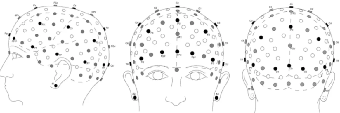
is located over the occipital area but on the left hemisphere, left to inion, However electrode Oz is over occipital area but in the middle, right above the inion. Based on the principles of the 10–20 system, a 10–10 system and a 10-5 system have been introduced as extensions to further promote standardization in high resolution EEG studies. This high density EEG electrode placement can help pinpoint more accurately the brain region contributing to the recording at a given electrode. This is known as source localization [79].

Figure 2-7(b): Selection of 10–10 electrode positions in a realistic display, lateral, frontal and posterior views. The head and brain contours based on typical models. Black circles indicate positions of the original 10–20

system, grey circles indicate additional positions in the 10–10 extension [79]

2.4.2. Mono-polar and bipolar recordings

EEG is a measurement of potential changes over time in a basic electric circuit conducting between signal (active) electrode and reference electrode. For getting a differential voltage, an extra third electrode called the ground electrode, is needed by the amplifiers to subtract the active and reference channels from it.

Reference electrode(s) must be placed on the parts of the body where the electrical potential remains fairly constant, so the most preferred reference is linked ears due to the relative electrical inactivity, ease of use and symmetry which prevents a hemispheric bias being introduced. This way of montage is called mono-polar. Another type of electrodes montage is bipolar recording. They are differential measurements that are made between successive pairs of electrodes. Closely linked bipolar recordings are superior to mono-polar recordings because they are less affected by some artifacts, particularly ECG, due to the differential cancelling out of signals similarly picked up at the pair of electrodes, so each electrode is referenced

to a neighbor electrode or to common reference electrode. However, in terms of placement and spatial resolution, the mono-polar is more favorable [79],[89].

2.6. EEG signals used to drive BCIs

The EEG recorded brain waves originate from a multitude of different neural communities from various regions of the brain. These neural communities produce electrical contributions or components that can differ by a number of characteristics such as topographic location, firing rate (frequency), amplitude, latency etc.

Here are the main EEG patterns used to drive BCIs:

Table 2-3: EEG signals to drive BCIs [5], [35]

Signal

Short Description

ERD/ERS A voluntary movement results in a circumscribed Event Related De-synchronization (ERD) in the µ and lower beta bands. It begins in the contra-lateral rolandic region about 2 s prior to the onset of a movement and becomes bilaterally symmetrical immediately before execution of movement. The power in the brain rhythms increases with an Event-Related Synchronization (ERS). It is dominant ipsilaterally during and contra-laterally after the movement over sensorimotor area and reaches a maximum around 600 ms after movement offset.

MRP MRPs are low-frequency potentials that start about 1–1.5 s before a

movement. They have bilateral distribution and present maximum amplitude at the vertex. Close to the movement, they become contra-laterally preponderant

SCPs Slow Cortical Potentials are slow, non-movement potential changes generated by the subject. They reflect changes in cortical polarization of the EEG lasting from 300 ms up to several seconds. Functionally, SCP reflects a threshold regularization mechanism for local excitatory mobilization

visual stimulus. These potentials are more prominent in the occipital area.

SSVEP Steady State Visual Evoked Potentials (SSVEP) are generated in response to a flashing visual stimulus with a repetition frequency greater than 6 Hz. These potentials are at the same frequency of the stimulus and they are more prominent in the occipital area.

SSAEP Steady State Auditory Event Potentials (SSAEP) are sustained responses to continuous trains of click stimuli, tone pulses or

amplitude-modulated tones, with a repetition or modulation rate between 20 and 100 Hz. The resulting brain response can be localized in the primary auditory cortex and are frequency-matched and phase-locked to the modulation.

P300 Infrequent or particularly significant auditory, visual, or somatosensory stimuli, when interspersed with frequent or routine stimuli, typically evoke in the EEG over the parietal cortex a positive peak at about 300 ms after the stimulus is received. This peak is called P300

Response to mental tasks

BCI systems based on non-movement mental tasks assume that

different mental tasks (e.g., solving a multiplication problem, imagining a 3D object, and mental counting) lead to distinct, task-specific

Chapter 3

Brain Computer Interfaces (BCIs)

3.1. Introduction

A brain-computer interface (BCI) is an artificial communication system that passes the brain’s normal output pathways of peripheral nerves and muscles, measures brain activity associated with the user's voluntary intend and desire, and

characterizes these intentions with signal Digital Signal Processing (DSP) algorithms, in order to translate those intentions into a control signal that commands a device to act accordingly with those intentions only and without presence of any muscle activity[8].

BCIs use EEG system where the computer processes the EEG signals and use them to accomplish tasks such as communication and environmental control. Due to EEG complexity and noisiness, which in turn complicates processing those signals, these factors make using those signals for performing a simple task, such as moving a cursor left or right a very hard and challenging work, which makes BCIs slow in comparison with normal human actions.

EEG signals are too complex to be analyzed in terms of underlying neural events. EEG signals are in micro-volts and may be affected by muscular artifacts as eye and jaw movements. Also, a potential change at the scalp could be caused by the same polarity produced near the surface of the cortex, but it may also be caused by a potential change of the opposite polarity occurring at cell bodies deeper in the cortex. Excitation in one place cannot be distinguished from inhibition in another place and thus individual thoughts cannot be divined [6].

Individual thoughts cannot be picked up and are probably not even correlated with the ongoing EEG activity. It is possible for an individual to be trained to produce a reliable signal or an individual may have a reliable response to a specific stimulus in a specific context. BCIs make use of such signals and if reactions to computer

switch or a television set. If individuals may be trained to produce reliable signals that may be separated from ongoing EEG activity, then these signals may be used.[6] On the other hand, recent advances in computers and signal processing have opened up a new generation of research on real-time EEG signal analysis and BCIs. With a small comparison between the first BCI presented by Dr. Grey Walter in 1964, and the new state-of-the-art BCIs presented by Wolpaw in 2010, we can see how computers have become fast enough to handle the real-time old constraints of BCI signal processing.

3.2. BCI design approaches: Pattern Recognition Vs Operant

conditioning

In Pattern recognition approach (PR), the BCI recognizes the characteristic EEG in response to performing a cognitive mental task like motor imagery, visual, arithmetic and baseline tasks [79]. It is mainly used in SSEVP-BCI.

However, Operant conditioning approach (OC) requires the user to perform lengthy training sessions in a biofeedback environment to master the skill of being able to

self-regulate one’s EEG, and is mainly used for ERD-BCI [79],[86].

3.3. BCI control approaches: Synchronous Vs Asynchronous

Synchronous BCI approach implies that the user can interact with the targeted application only during specific time periods triggered by external audio/visual stimuli and imposed by the computer system, whereas in Asynchronous BCI, the user willingly decides when to perform a mental task and at any time [24].

However, designing an asynchronous BCI is much harder than designing a

synchronous BCI. In the latter, the system is programmed to know when the mental states should be recognized and analyzes EEG only in predefined time windows, however, with a self-paced BCI; the system has to analyze EEG continuously in order to determine whether the user is trying to interact with the system by performing a

mental task. So it requires computations much more than synchronous BCI does which leads to less accuracy due to the high amount of data being processed. This in turn limits the speed of command generation for such an approach [24].

3.4. BCI framework

Figure 3-1: BCI framework [24]

The design of a BCI system consists of six main stages: the acquisition of EEG signals, pre-processing the signals, feature extraction and selection, classification and translation into a command or a control signal, and finally to feedback the subject with a desired action [5],[24].

A BCI system commences with acquisition of brain signals, which is done via an EEG system with one up-to 256 electrodes. Each mental activity generates specific EEG signals related to this task topographically and rhythmically, so numbers and locations of electrodes (according to the 10-20 system) are related to the task the designer wants to achieve with a BCI.

The signals are then amplified, filtered, epoched (in order to center and maximize the information of the data in the specific related rhythm), A/D converted and passed through an artifact removal algorithms (de-noised) in what is known as pre-processing stage [79]. The main goal of this stage is to improve the signal-to-noise ratio (SNR) by cleaning the EEG signals and removing all irrelevant information, such as the electrical activity of the eyes (EOG: ElectroOcculoGram), the muscles (EMG: Electromyogram) and the power line network, which have an amplitude much larger

than the one of EEG signals. Thus the pre-processing stage reduces the amount of data for the next stages. This reduction is essential, because EEG signals ports a large amount of data which make it harder to work with, so focusing on a smaller amount of data that has the relevant information, would facilitate the design [79].

After cleaning the signals from irrelevant information, the relevant information, which is known in the world of BCI as features, needs to be extracted [5]. The feature extraction represents the resultant signals as feature values that are related to the underlying neurological mechanism generated by the user's brain for control. These features can be for example the magnitude at a specific frequency range. Features are extracted with DSP algorithms and assembled into a feature vector. Hence, feature extraction is the stage where DSP algorithms are applied in order to convert one or several signals into a feature vector [5],[24].

This stage may results in too many irrelevant overlapping feature vectors which increase the computational complexity, so feature selection with DSP algorithms may be applied for optimization [32].

In the next stage, the classification stage, classification algorithms are applied to categorize different brain patterns and features from the feature vectors [5],[24], where each classified features will be translated into a distinct control signal related to the underlying brain pattern. In this final stage, control signals instruct the device to act and feedback the user. Each control signal represents a specific brain pattern related to the user's intention, so the device will act accordingly with the identified user’s intention. The BCI performance is determined in terms of classification accuracy [8], computational efficiency and complexity [79].

Consequently, designing a BCI is a complex and challenging task which requires multidisciplinary expertise such as programming, signal processing, neurosciences and psychology [8]. To complete a BCI design, two phases are essential: 1) an offline training phase which calibrates the system. An experimental paradigm [14] is implemented to guide the user on how to generate the characteristics EEGs. It is mainly characterized by its duration, repetitiveness, pause between trials and complexity of the mental task. The training paradigm is generally done without the feedback stage, even thought that there is some evidence that a continuous or

discrete visual representation of the feedback signal, such as a 3D video game or virtual reality environment, may facilitate learning to use a BCI [42].

2) an online phase which uses parameters from phase 1 in the BCI to distinguish mental states and feedback the user accordingly.

Chapter 4

BCI signal processing

4.1. Pre-processing Methods

4.1.1. Temporal filters

Low-pass or band-pass filters are generally used in order to restrict the analysis to frequency bands known as representing neurophysiological signals [24]. For Instance, BCI based on sensorimotor rhythms generally band-pass filter the data in the 8-30Hz frequency band, as this band contains both the μ and ß rhythms. This temporal filter can also remove various undesired effects such as slow variations of the EEG signal (which can be due, for instance, to electrode polarization) or power-line interference (60 Hz in Quebec). Hence, such a filtering is generally achieved using Discrete Fourier Transform (DFT) or using Finite Impulse Response (FIR) or Infinite Impulse Response (IIR) filters (Butterworth, Tchebychev or elliptic IIR filters) [24].

4.1.2. Spatial filters

Spatial filters are used to isolate the relevant spatial information embedded in the signals. This is achieved by selecting the electrodes for which we know they are measuring the relevant brain signals, and ignoring other electrodes [24]. The most popular spatial filter is the Common Average Reference (CAR) which is obtained as follows:

= − ( )

Where and Vi are the ith electrode potential, after and before filtering

respectively, and Ne is the number of electrodes used [24]. Thus, with the CAR filter,

4.1.3. Independent Component Analysis (ICA)

ICA is a method for separating a multivariate signal into additive subcomponents supposing the mutual statistical independence of the non-Gaussian source signals [24]. It is a special case of blind source separation.

When the independence assumption is correct, blind ICA separation of a mixed signal gives very good results. It is also used for signals that are not supposed to be generated by a mixing for analysis purposes. A simple application of ICA is the "cocktail party problem", where the underlying speech signals are separated from a sample data consisting of people talking simultaneously in a room.

Blind signal separation, also known as blind source separation, is the separation of a set of signals from a set of mixed signals, without the aid of information (or with very little information) about the source signals or the mixing process [20], [55].

Blind signal separation relies on the assumption that the source signals do not correlate with each other. For example, the signals may be mutually statistically independent or de-correlated. Blind signal separation thus separates a set of signals into a set of other signals, such that the regularity of each resulting signal is

maximized, and the regularity between the signals is minimized (i.e. statistical independence is maximized).

4.1.4. Common Spatial Patterns (CSP)

This method is based on the decomposition of the EEG signals into spatial patterns selected in order to maximize the differences between the classes involved once the data have been projected onto these patterns [91],[24],[55]. Determining these patterns is performed using a joint diagonalization of the covariance matrices of the EEG signals from each class. With the projection matrix W, the original EEG can be transformed into uncorrelated components:

Z=WX (2)

Z can be seen as EEG source components, and the original EEG X can be

reconstructed by

Where W-1_{is the inverse matrix of W. the columns of W}-1_{are spatial patterns, which}

can be considered as EEG source distribution vectors. The first and last columns are the most important patterns that explain the largest variance of one task and the smallest variance of the other [91].

4.2. Feature extraction

4.2.1. Temporal Methods

4.2.1.1. Signal amplitude

The simplest (but still efficient) temporal information that could be extracted is the time course of the EEG signal amplitude. Thus, the raw amplitudes of the signals from the different electrodes, possibly preprocessed, are simply concatenated into a feature vector before being passed as input to a classification algorithm. In such a case, the amount of data used is generally reduced by preprocessing methods such as spatial filtering or sub sampling. This kind of feature extraction is one of the most used for the classification of P300.

4.2.1.2. Band power features [35],[41]

For EEG data, Band-pass filtering of each trial, squaring of samples and averaging of N trials results in a time course of instantaneous band power [41]. It is also possible to log-transform this value in order to have features with a distribution close to the normal distribution. The power is calculated as:

= ( , ) ( )

where P(j) = averaged power estimation of band-pass filtered data (averaged over all trials), xf(i,j)=j-th sample of the i-th trial of the band-pass filtered data[25].

Then, The ERD is quantified as the percentage change of the power (A(j)) at each sample point or an average of some samples relative to the average power in a reference interval:

%( )= ( )−

% ( )

= ( )

where R = average power in reference interval, averaged over k samples, and A(j) = power at the j-th sample [25].

4.2.1.3. Autoregressive (AR) Parametric model

Autoregressive (AR) methods assume that EEG signal y(t), measured at time t, can be modeled as a formula, or a polynomial model that is optimally fitted into a time series, and that attempt to predict an output of a system based on the previous

outputs, to which we can add a noise term et (generally a Gaussian white noise):

y (t)=-a

y(t-1)- …- a

(t-n

)+ e(t) (7)

Where a1,a2…..an are the autoregressive parameters which are generally used as

features for BCI to distinguish one time-series from another, and n is the model order [79], e(t) is a purely random (white noise) process with zero mean and

variance σ2n . n(t) is uncorrelated with the signal, and the cross-covariance E{Xt* Nt-k}

is zero for every k. In [79] the author mentioned that Mc Ewen et al. showed that 80-90% of EEG segments of duration 4-5 seconds can be modeled as being Gaussian. The AR model can be rephrased in the frequency domain as a white noise source

driving a spectral shaping network A−1 (z)[79].

Figure 4-2 AR Model [79]

Several extensions to the AR have been proposed [24]: 1. AAR (Adaptive Auto-Regression)

2. ARX (Auto-Regression with exogenous input) 3. ARMA (Auto-Regression with Moving Average)

4. ARMAX (Auto-Regression with Moving Average and exogenous input) Using an AR Moving Average (ARMA) as the Exogenous input has proved to better model the underlying event-related potential amidst the background EEG offering improved classification rates [79]. It makes the distinction between the ERP and background neuronal activity contributing to the single trial EEG recording, but requires more computational time and processing capabilities due to its iteration functionality. ARX, an extension of AR modeling, involves the introduction of an

exogenous input assumed to be a contributory signal to the overall signal being modeled. Its pole-zero filtered contribution and the AR noise estimate combine to form the forward prediction estimate of the overall recorded EEG signal. The ARX filter coefficients are used as input features to characterize the single-trial EEG. The ARX method of modeling both the signal ERP and the noise (background EEG) is more physiologically reasonable than modeling the noise alone as ongoing EEG contributions from neighboring neural populations contribute mostly to the

background noise [19]. Ensemble averaging over a large number of trials exposes the underlying ERP that is hidden amidst background EEG by averaging out this random neuronal noise.

The EEG can be expressed by means of the following equation (assuming a linear relationship):

( ) = ( ) + ( ) + ( ) 0 ≤ ≤ (8)

where: ( )is the scalp recorded EEG response prior to the onset of movement, ( ) is the useful signal corresponding to the ERP attained by ensemble averaging across

preceding trials [19], ( )

generated by a combination of all possible artifacts. T is the duration of each fixed length trial epoch. Alternatively, the ARX model can be extended for artifact filtering by introducing additional noise modeling stages to filter the acquired signal y(t) , resulting in increased exogenous inputs.

Figure 4-3 ARX Model [79]

The basic ARX model, in terms of the shift operator q, and assuming a sampling interval of one unit, is as follows

( ) ( ) = ( ) ( ) + ( ) ( )

( ) = − ( − ) − ⋯ − ( − ) + ( − ) + ⋯ + ( − − ) + ( ) ( )

Where

n

n

ARX models are usually used as features in the classification. This feature extraction technique is impractical for a large number of electrodes due to the resultant large feature vector dimensionality and resulting computational demands. Different model orders are tested to select the optimum model order that represents the input data. This selection is based on the standard prediction error method over the state-space model. State-space models are common representations of dynamical models, and they describe the same type of linear difference relationship between the inputs and the outputs as in the AR and ARX model [50].These models use state variables to describe the system by a set of first-order differential or difference equations, rather than by one or more nth-order differential or difference equations. They can be reconstructed from the measured input-output data, but are not

themselves measured during an experiment [50]

( ) = ( ) + ( ) + ( )

( ) = ( ) + ( ) + ( ) (11)

A, B, C, D, and K are state-space matrices. u(t) is the input, y(t) is the output, e(t) is

the disturbance and x(t) is the vector of orders states. All the entries of A, B, C, and K are free estimation parameters. The elements of the D matrix, however, are fixed to zero. That is, there is no feed-through. For ARX model order selection, the Akaike Information Criterion (AIC) was applied for this study [50]. In this method, the input was assumed to have Gaussian statistics, thus the AIC for an AR process is as follows

= ( ) + ( )

Where is the loss function, is the modeling error, is the AR model order, and is the number of data samples.