Design of Load Shedding Schemes against Voltage Instability

Design

of

Load Shedding Schemes against Voltage Instability

C.

Moors

D.

LeCebvre

T.

Van

Cutsem

Research engineer, FRIA University of Li&ge, Institut Montefiore

Sart Tilman 828. B-4000 tibge, Belgium

Research director, FNRS

University of Liege, Institut Montefiore

Sart Tilman B28, B-4000 Liege, Belgium Hydro-QUebec, Division Transhergie

CP 10000 Montreal (QC). Canada

Abstract. This paper proposes a methodology for the design of au-

tomatic load shedding against long-term voltage instability. In a first step, a set of training scenarios is set up, corresponding to various oper-

ating conditions and disturbances. Each scenario is analyzed to deter-

mine the minimal load shedding which stabilizes the system, with due consideration for the shedding location and delay. In a second step, the parameters of a closed-loop undervoltage load shedding scheme are de-

termined so as to: (i) approach as closely as possible the optimal shed-

dings computed in the first step, over the whole set of scenarios; (ii)

stabilize the system in all the unstable scenarios and (iii) shed no load

in the stable ones. The corresponding optimization problem is solved

using a (micro-)Genetic Algorithm. A detailed example is given on the

Hydro-Quebec system in which load shedding is presently planned.

Keywords. System stability and analysis, voltage stabilization and con-

trol, genetic algorithms.

I. INTRODUCTION

There are two lines of defence against incidents which jeop- ardize the stability of power systems:

*preventively: analyze the system security margins with respect

to credible contingencies, i.e. incidents with a reasonable prob-

ability of occurrence, and take appropriate preventive actions to restore sufficient margins when needed;

0 correctively: implement automatic corrective actions, through

System Protection Schemes

(SPS)’

to face the more severe, but

less likely incidents.

The preventive security criteria usually require that the sys- tem remains stable after any credible contingency, without the help of corrective actions. The main reason is that these ac- tions usually affect the system generation and/or load, which is acceptable only in the presence of severe disturbances.

The present paper concentrates on long-term voltage stabil- ity, driven by Load Tap Changers (LTCs), generator OverExci-

tation Limiters (OELs), switched shunt compensation, restora-

tive loads, and possibly secondary voltage control. This type of

instability has become a major threat in many systems [l, 21.

‘also referred to as Special Protection Schemes

0-7803-5935-6/00/$10.00 (c) 2000 IEEE 1495

Since long-term voltage instability is triggered mainly by the

loss of generation or transmission facilities,

“N-1”

contingen-

cies corresponding to the loss of a single equipment are usually considered in preventive security analysis. On the other hand,

N-2 and more severe disturbances should be counteracted by

an

SPS.

While it must be used in the last resort and to the least extent, automatic load shedding is very effective in this respect. A few undervoltage load shedding schemes have been imple-

mented throughout the world (e.g. [3]. Beside time-domain nu-

merical simulation, methods have been proposed to identify the best location, time and amount of shedding in a given unstable

scenario (e.g [4,5]). There is however a need for a methodology

to help planners in designing this type of SPS.

This paper proposes such a methodology. The latter consists of two steps:

in the first step, a set of mining scenarios is set up, cor- responding to various operating conditions and various distur- bances. Each scenario is analyzed to determine the minimal load shedding which stabilizes the system, with due considera- tion for the shedding delay;

in the second step, the parameters of a closed-loop protection are determined in order to approach as closely as possible the optimal sheddings computed in the first step, over the whole set of scenarios. A genetic algorithm is used to this purpose.

The paper is organized as follows. Section I1 describes how

the minimal load shedding is determined when analyzing the

unstable scenarios in the first step. Section I11 deals with the

second step of the procedure. Section IV provides a rather com- plex example taken from the Hydro-QuCbec system, in which an undervoltage load shedding scheme is planned. The paper ends up with some concluding remarks.

11.

DETERMINATION

OF

OPTIMAL LOAD SHEDDING

Location, amount and delay are the three main characteris- tics of load shedding. Obviously the amount of load shedding should be minimal.

For a given shedding delay and location, the minimal amount

of shedding Pmin can be simply determined by binary or incre-

mental search, resorting to time-domain simulations to check

the system behaviour.

As

far as long-term voltage stability is

concerned, the computing times can be dramatically reduced by using the Quasi Steady-State (QSS) simulation techique. This well-documented approach is based on time decomposition and consists of replacing the short-term dynamics by equilibrium

The next point is to determine which delay and location yield

the smallest amount Pmin. These two problems are discussed

separately hereafter.

A. Optimizing with respect to the shedding delay

The main motivation for delaying load shedding is to ascer-

tain that the system is indeed voltage unstable, and hence to

avoid shedding load unduly.

The influence of the delay T (counted from the disturbance in-

ception) on the minimal amount of power to shed

Pmin

can

be

easily established for the simple two-bus system of Fig.

1

.a. In

this system, the load is assumed to obey the well-known expo- nential model in the short term and to restore to constapt power

in the long term, owing to the LTC effect. The Pmrn vs. T

characteristic is shown with solid line in Fig. 1.b and is easily

explained as follows [ 5 ] :

-

the minimal amount of load power to shed does not vary as

far as load shedding takes place before the critical time -rc. This

amount, denoted P*, is the load decrease just needed to create

a long-term equilibrium in the post-contingency configuration;

-

if the shedding takes place after T ~ , more load has to be shed;

this is a matter of attraction towards the newly created long-term equilibrium.

Note however that a severe disturbance may yield the char- acteristic shown with dashed line in Fig. 1.b. in which Pmin increases right away after the disturbance.

7

I >

Tc

Figure 1 : Theoretical shedding characteristic of a two-bus system

According to the authors’ experience, large real-life systems

have Pmin vs. T characteristics quite close to that of Fig. 1, as

far as the long-term dynamics are governed by OELs, LTCs and

secondary voltage control (if any) [5].

On the other hand, the characteristic may change when other

post-contingency controls “compete” with load shedding. In

this case, it may be advantageous to delay load shedding so that

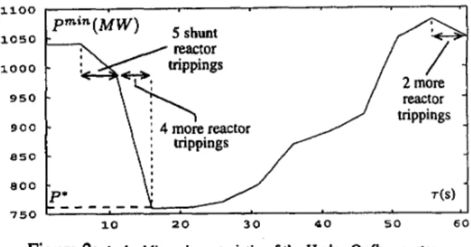
these controls act first and hence less load is shed. An example is provided in Fig. 2, relative to the Hydro-QuCbec system con- sidered in Section IV. In this system, automatic shunt reactor tripping significantly contributes to stabilizing the system in its post-contingency configuration. The figure shows that 280 MW

load are saved when the shedding is delayed by 16 seconds, al-

lowing 2970 Mvar to be tripped before load is shed.

In the design of a load shedding protection, we will use the

minimum P* as a target value. When the Pmin vs. T char-

acteristic is of the type shown in Fig. 1, P* is merely taken as

the value of Pmin for a load shedding taking place very shortly

after the disturbance (ideally T = 0). When a more complex

characteristic is expected, such as in Fig. 2, P* is determined as

1100 I I 1050 1000 9 5 0 9 0 0 8 5 0 reactor trippings : 4 more reactor trippings T ( S ) 8 0 0 7 5 0 2 0 3 0 4 0 5 0 6 0 10

Figure 2: A shedding characteristic of the Hydro-Qukbec system

the minimum value of Pmin over a speficied interval of T .

B.

Optimizing with respect to the shedding location.

There are basically two proven approaches to identify the op- timal location:

a small-disturbance analysis coupled with time-domuin simu- lation [5]. Along the unstable trajectory provided by a time-

domain method, sensitivity analysis is used to identify the criti- cal point, at which the eigenvector corresponding to the (almost) zero eigenvalue is computed. This information allows to obtain a ranking of load buses with respect to the efficiency of load

shedding. A given amount of load shedding is distributed over

the buses in this order, taking into account the interruptible frac- tion of each load;

e Optimal Power Flow (OPF) [4]. The objective is to minimize the amount of load shedding, taking into account the constraints stemming from the load flow equations, the generator reactive limits and the interruptible fraction of each load. This approach provides the optimal location and the minimal amount of load

shedding in a single step.

In the first approach, a coupling between time-domain sim-

ulation and small-disturbance analysis is necessary. This cou-

pling in easier with

Q S S

simulation which is free from short-

term transients.

In the OPF approach, it is possible to require the system

to satisfy some operating constraints, in addition to being sta- ble. On the other hand, the OPF relies on a simplified system

modelling (typically load flow equations) and does not allow to

check the delay aspects discussed in the previous section. To this purpose, a time-domain method is needed anyway.

111. DESIGN OF THE LOAD SHEDDING

PROTECTION

A. Scenario analysis

As already mentioned, the first step of our approach consists

in setting up a set of 8 training scenarios, corresponding to vari-

ous topologies, load levels, generation schemes, and contingen- cies.

In principle all the scenarios to be dealt with by a single

protection should involve the same weak area of the system;

in other words, the instability modes and hence the optimal

shedding locations should be rather close for all the unstable scenarios of the set. Therefore, we assume that a common bus ranking can be set up for all of them. Once this ranking has

been identified, the minimal amount of load shedding

Pi*

is de-

termined for each scenario

(i

= 1,

.

. .

,

s), according to the pro- cedure described in the previous section.

B.

Logic of the load shedding protection

Generally speaking SPSs can be classified into :

e event-based vs. response-based protections. The former

rely on the direct identification of the disturbance (e.g. circuit breaker operation signals, etc.), while the latter rely on the effect of the disturbance on measured system variables. Event-based protections are needed when speed of action is essential. This is usually not the case for long-term voltage instability; hence, a response-based protection will be considered in the sequel. We

assume that a single signal V is monitored. This is typically the

average voltage over several transmission buses in the load

area

of concern. In practice, other measurements can enter the logic,

such as the reactive reserve on neighbouring generators, etc. but

this is not considered here for simplicity.

e open-loop vs. closed-loop protections. By closed-loop we

mean a protection which takes successive actions, each on the

basis of the signal V resulting from the previous actions. In

other words, the signal V stemming from the system is fed back

to the protection. This closed-loop design is preferred as being

more robust with respect to modelling and operating condition uncertainties.

In accordance with the above remarks, we consider a protec-

tion based on

k

rules of the type:

ifV is smaller than

Kmin

during di seconds, shed AFi MW

The number

k

of rules is decided

a

priori; in practice it is typi-

cally equal to 2 or 3.

Note that such a protection operates in closed loop since V

is continuously measured and the same rule may trigger several successive load sheddings in time.

C. Statement of the design problem

Given the s training scenarios, the problem is to determine

the 3k-dimensional vector of unknowns:

x = [VImin, dl AP1,

. . .

Vkmin, d k , APk] (1)

such that the following requirements are met:

1. the amount of load shedding must be as close as possible to

the minimal amount P: (i = 1,.

.

.

,

8 ) determined in the first

step;

2. all unstable scenarios must be saved (SPS dependability);

3. no load must be shed in a stable scenario (SPS security);

4. optionally, some other constraints can be imposed. For in-

stance, the distribution voltages should not stay below some threshold for more than some time.

This can be translated into an optimization problem: mini-

mize the discrepancies

Pth(x)

-

Pi*, where

P / h ( ~ )

is the total

load power shed in the i-th scenario, for a given protection set-

ting x. W O objectives have been considered:

min

C [ P ~ ~ ( X )

-

P?

+

pi(x)] (2)

or min

m*[P/"(x)

-

P

:

+

pi(x)] (3)

i a

where the sum and the max extend over the unstable scenarios

and pi(x) is a penalty term accounting for the violation of the

above requirements, as described hereafter.

When the system is unstable (requirement 2 violated), trans-

mission voltages eventually become smaller than some thresh- old VloW. Denoting by tlow the time at which this occurs', the penalty takes on the form:

c1

>>

0 c2

>

0 (4)

Cl

t1ow

+

c2

Pi =

When an amount

T h

is shed in a stable case (requirement 3

violated), the penalty term takes on the form:

pi = kP,"h

k

>>

1 ( 5 )

Let tre, be the recovery time, i.e. the time at which voltages

are again larger than a specified value Vmin. Requirement 4

consists in specifying that t r e e is smaller than a given value

tz".

If this does not hold, the penalty is taken as:

pi = C 3 ( t r e c

- tz:")

C 3

>>

O ( 6 )

Note that with the above penalties, the more dangerous a sit-

uation (i.e. the shorter tlowr the larger P t h or tree), the higher

the penalty. This is expected to provide the optimization method with information on how to improve the parameters.

The optimization problem (2-6) is complex. Indeed, both

P t h

and pi must be determined from time-domain simulations and hence, explicit analytical expressions cannot be established.

Moreover, they vary with x in a discontinuous manner. This

prevents from using classical analytical optimization methods. Also, multiple local minima are expected. A "controlled ran-

dom search" method, in the form of a Genetic Algorithm, seems

better suited to this combinatorial optimization problem.

0-7803-5935-6/00/$10.00 (c) 2000 IEEE 1497

D. Optimization through a micro-Genetic Algorithm

Genetic algorithms (GAS) are optimization techniques in-

spired by the theory of evolution 181. They combine survival

of the fittest among string structures with a structured yet ran- domized information exchange to form a search algorithm with

some of the innovative flair of human search. They allow to find

near-optimum solutions of multimodal objective functions.

The basic principle of GA methods is to make evolve a pop-

ulation of potential solutions to a given optimization problem.

Specifically, they operate on structures, which are encoded rep- resentations of the solution (e.g. strings of bits from a binary al- phabet). Each solution is associated with afitness value, which

*In a long-term voltage unstable situation. the system may finally loose Its

short-term equilibrium, which corresponds to a fast collapse When the QSS

technique is used, the simulation cannot proceed. If this occurs before the V[O"

is simply the corresponding value of the objective function to be optimized. When each structure in the population has been eval- uated, a new population of candidate solutions is formed in two

steps. First, structures in the current population are selected for

replication based on their relative fitness. The higher the fitness

value of an individual, the higher its representation in the subse-

quent generation. Next, the selected structures are altered using

crossover and mutation operators. The crossover operator com-

bines the features of two parent structures to form two similar

children by exchanging parts of the parents’ strings. The muta-

tion operator, which alters randomly one or more components

of a selected structure, provides the way to introduce new ge- netic materials. Mutation usually ensures the reachability of all points in the search space, preventing premature convergence. The resulting children are then evaluated and inserted back into the population, replacing older members.

Progressively, this process improves the performances of the population through the generations, until no better individual can be found. At that stage, the algorithm has converged, and most of the individuals in the population are almost identical. While randomized, genetic algorithms are no simple random walk. They efficiently exploit historical information to specu- late on new search points with expected improved performance. In this work, we have used a micro-Genetic Algorithm (PGA) (9, lo]. Compared to GAS, pGAs have a much smaller popu- lation size (typically 5 individuals vs. 30 to 200 individuals

for GAS). Moreover, the mutation operator is replaced by a

random insertion of new individuals, once convergence of the micro population has been detected. Studies have shown that pGAs reach the near-optimal region much earlier.

E. On the choice of training scenarios

Attention must be paid to the design of the training scenarios. This task requires a good engineering knowledge of the system. Although the choice of scenarios depends to a large extent on

system specifics, the following appear as important guidelines:

0 in order to meet requirement 3 of Section UI.C, the training set

should include a significant number of marginally stable cases,

on which the protection must be trained not to act;

0 the Pc values should be rather uniformly distributed in be-

tween the marginally and the most severely unstable cases;

0 with the protection already trained not to act in marginally

stable cases, more stable scenarios need not be considered.

IV.

RESULTS ON THE HYDRO-QUEBEC SYSTEM

A. Voltage stability of the Hydro-Qu6bec system

The Hydro-Qutbec system is characterized by great distances (more than 1000 km) between the large hydro generation areas (James Bay, Churchill Falls and Manic-Outardes) and the main load center (around Montreal and Quebec City). Accordingly, the company has developed an extensive 735-kV transmission system, whose lines are located along two main axes. This sys-

tem is angle stability limited in the North, voltage stability lim-

ited in the South (near the load center). Frequency stability is

also a concern due to the system interconnection through DC

links only, as well as the sensitivity of loads to voltage.

In the recent years, Hydro-Quebec has undertaken a major program to upgrade the reliability of its transmission system. In particular a defence plan is being deployed against extreme contingencies [7]. This includes generation rejection and re- mote load shedding, automatic shunt reactor switching, under-

frequency load shedding and in a near future, undervoltage load

shedding.

Beside static var compensators and synchronous condensers, the automatic shunt reactor switching devices, known under the

French acronym

MAIS,

play an important r61e in voltage con-

trol [ 111. These devices, in operation since early 1997, are now

available in 22 735-kV substations and control a large part of the total 25,500 Mvar shunt compensation. Each MAIS relies on the local voltage, the coordination between substations be- ing performed through the switching delays. While fast-acting MAIS can improve transient (angle) stability, slower MAIS sig- nificantly contribute to voltage stability.

Preventive security assessment is also a major concern.

Presently, secure operation limits are determined in operational

planning. with the help of ASTRE, the QSS simulation program developed at the University of Li6ge [2, 63. This fast tool has

been used in the present study. The corresponding model in-

cludes around 550 buses, 100 generators and 230 LTCs. The

total load is around 33,000 M W .

B.

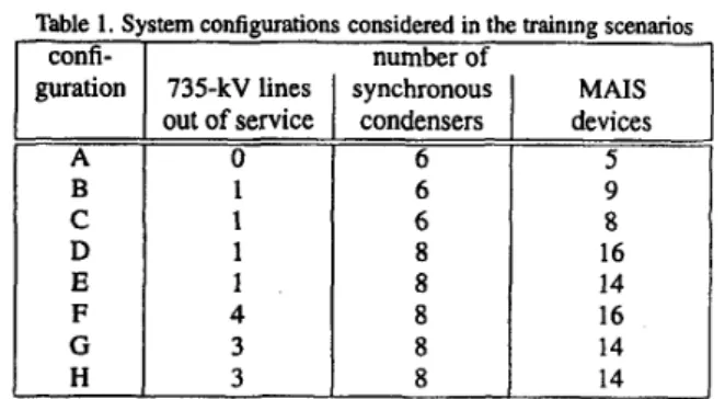
Training scenarios and main protection parameters

The study reported in this paper involves 8 system configura-

tions, summarized in Table 1.

Table 1. System configurations considered in the training scenarios

confi- guration 735-kV lines out of service 4 3 3 number of synchronous condensers 6 6 6 8 8 8 8 8 MAIS devices 5 9 8 16 14 16 14 14

Table 2 details the 36 scenarios finally selected. They involve

N- 1, N-2 and N-3 contingencies, respectively. In accordance

with the standard operating rules, the system is stable follow- ing any N-1 incident. The MAIS devices can be used to this purpose.

In each unstable scenario, the best load shedding location has been identified. Therefrom, a common ranking of load buses

has been set up. For simplicity, each load is assumed fully in-

terruptible. Using this bus ranking, the minimal amount of load

shedding P,? required to stabilize the system has been deter-

mined in the 19 unstable scenarios. The values, computed with

an accuracy of 10 M W , are given in Table 2. The most severe

incident requires to shed load at 8 buses.

-

No 1 2 3 4 5 6 I 8 9 10 1 1 12 13 14 15 16 17 18

-

(MW) 0 0 1090 460 110 1520 0 200 0 0 0 0 740 350 0 0 0 0

Table 2. Description of the 36

19 20 21 22 23 24 25 26 27 28 29 30 31 32 33 34 35 36

conf.

-

A A A A A A B B C D D D D D E E E E

-

incid.

-

type N- 1 N- 1 N-2 N-2 N-2 N-3 N- 1 N-2 N- 1 N- 1 N- 1 N-2 N-2 N-2 N- 1 N- 1 N-2 N-2

-

ining s conf. E E

F

F F F F G G G G G G H H H H H

-

-

Wios

incid.

-

type N-2 N-2 N- 1 N-2 N-2 N-2 N-2 N- 1 N- 1 N-2 N-2 N-2 N-2 N- 1 N- 1 N-2 N-2 N-2

pi*

(Mw) 890 890 0 0 1110 860 620 0 0 40 1790 880 760 0 0 310 730 600

The scenarios have been chosen according to the guidelines

of Section 1II.E: the 17 scenarios with Pi* = 0 are marginally

stable situations, while the nonzero values of Pi* range rather

uniformly in the [O 17901 MW interval.

As regards the protection, two rules

(k

= 2) have been con-

sidered. The measured signal V is the average voltage over five

735-kV buses in the MontrCal area. Both the “sum” (2) and

the “minmax” (3) objective functions have been considered, for

comparison purposes. Requirements 1 , 2 and 3 of Section 1II.C

have been taken into account. However, in accordance with Hydro-QuCbec planning rules, the 2nd requirement has been amended by allowing some (hopefully small) load shedding to take place after a stable but severe incident. The N-2 scenar-

ios Nb. 12, 17, 18 and 22 are concerned. The latter are merely

handled as unstable scenarios with P[ = 0 in (2,3).

For coding purposes, the unknown parameters x were dis-

cretized as follows:

0 threshold voltages Vmin : 8 (equally spaced) values in the

range [0.88 0.961 pu. The lower bound is the lowest admis-

sible voltage (the protection is expected to quickly increase V

above this value) while the upper bound is just smaller than the MAIS settings (typically 0.965-0.97 pu). The threshold varies by 0.01 1 pu steps, quite close to the measurement accuracy;

0 delays di : 16 values in the range [3 181 s. The lower bound

is the minimal delay to distinguish a voltage instability from a temporary undervoltage;

shedding steps AP, : 16 values in the range [50 8001 MW.

The lower bound is the minimum amount that can be tripped by opening distribution feeders, while the upper bound has been limited to avoid excessive load shedding.

The PGA software of [ 101 has been used.

C. Results and discussion

Minmax objective. The convergence of the PGA is declared after 700 generations, since no significant decrease in the ob- jective has been observed over the last 150 generations. The

0-7803-5935-6/00/$10.00 (c) 2000 IEEE 1499

obtained rules are:

RI:

if

V

<

0.95 p u during 11 seconds, shed 200 MW R2:

if

V

<

0.93 pu during 4 secondr, shed 500 MW

These results can be interpreted by inspection of QSS time

simulations of the type shown in Fig. 3, where a star indicates a

MAIS operation and Rx a load shedding due to rule Rx.

Rule R1 is used in the less severe unstable scenarios, for

which V does not decrease below 0.93 pu. The rather long de-

lay and the moderate shedding of R1 yield a good coordination

with the MAIS, which are given time to act. For instance, in the

case of Fig. 3.a, MAIS operation makes V recover before any

of the two rules is triggered. This avoids to shed load in stable scenarios. In the case of Fig. 3.b, load is shed only after all the MAIS have been exhausted.

Rule R2 is used in more severe scenarios, leading to a more

pronounced voltage drop. An example is provided in Fig. 3.c. Note that by not shedding too much load, the voltage remains below the settings of the MAIS and the latter operate, adding to the effect of load shedding.

The structure of the above rules is “classical” in the sense that the larger the voltage drop, the greater the action and the smaller

the delay to take this action. This is not the case when the sum

objective is minimised, as explained hereafter.

Sum objective. The convergence of the PGA is declared after

’SSO generations. The obtained rules are:

R1: if V

<

0.93 p u during 3 secon&, shed 350 MW

R2:

if V

<

0.91 p u during 4 seconds, shed 250 MW

The rather low voltage threshold of rule RI guarantees that no

load is shed in the stable scenarios (see for instance Fig. 3.d) and

allows more load to be shed (350 instead of 200 MW) without preventing the MAIS to operate.

The settings are such that rule R2 will be used only if the

voltage initially drops below 0.91 pu and stays below this value

after load has been shed by rule R1. Figure 3.e shows a scenario where the triggering of R1 inhibits R2, while in the more severe scenario of Fig. 3.f the two rules are triggered.

In other words, this protection behaves as if it had a single

rule but two shedding levels (350 and 600 M w resp.), according

to the disturbance severity.

Comparison. Figure 4 compares the performances of the two

protections in terms of “over-shedding” with respect to the op-

timal values Pt. The figure relates to the 17 unstable scenarios

and the 4 stable N-2 scenarios where load shedding is allowed

(in the remaining 15 stable cases, no load has been shed).

As can be seen, the sum objective yields perfect results in

some scenarios but also over-sheddings as large as 540 MW

in some others. Expectedly, the minmax objective yields more

uniform errors, with a maximum over-shedding of 360 MW, but

it is never perfect.

Finally, in scenarios 12,17, 18 and 22, the minmax protection sheds load in three cases while the sum protection never does.

V. CONCLUDING REMARKS

In this paper the design of automatic load shedding schemes is formulated as a combinatorial optimization problem solved

Figure 3: Average voltage in the M o n W area (pu) vs. time (s) in six scenarios stabilized by load shedding and shunt reactor tripping

-1

- WOE 1800 1400 120(1 1OW 8M) 600 400 2 M 0

T ”

3 4 5 L1 8 12 13 1 1 17 18 19 20 2 2 23 24 25 28 2 8 M 31 34 55 38 Ik.nulo.

Figure 4: Performances of the s u m and minmax objectives

by means of (micro-)genetic algorithms. This yields optimized

rules which can be easily implemented and interpreted. Obviously, many aspects remain to be investigated. Let

us quote non exhaustively: a more in-depth tuning of the

(micro-)genetic algorithm parameters and the development of techniques to speed up computations. These improvements would allow to handle a larger number of scenarios (e.g. more system configurations and more incidents), a wider range of possible load behaviours (to take into account the uncertainty in their modelling) and eventually more detailed time simula-

tions (in order to handle, for instance, short-term voltage insta-

bility situations, or to coordinate load shedding with other, fast countermeasures).

Although Genetic Algorithms have been chosen for their proven ability to deal with complex problems, alternative com- binatorial optimization methods are worth being considered.

In spite of the above expected improvements, the approach has already given very satisfactory results. In the Hydro-Quebec system, for instance, it is already helping planners in the com-

plex task of designing a robust system protection scheme.

VI. REFERENCES

0-7803-5935-6/00/$10.00 (c) 2000 IEEE 1500

[l] C. W. Taylor, Power System Voltage Stability. Mffiraw Hill. EPRl Power System Engineering series. 1994

[2] T. Van Cutsem, C. Voumas, Voltage Stability of Electric Power Systems, Boston, Kluwer Academic Publishers, 1998

[3] C. W. Taylor, “Concepts of undervoltage load shedding for voltage stability”.

IEEE Trans. on Power Delivery. Vol. 7. pp. 480-488, 1992

[4] S. Granville. J.C.O. Mello, A.C.G. Melo, “Application of interior paint meth- ods to power flow solvability”, IEEE Trans. on Power Systems, Vol. 11, pp,

[SI C. Moors, T. Van Cutsem, “Determination of Optimal Load Shedding against Voltage Instability”, 13th PSCC Proceedings, Trondheim, 1999. pp. 993-1000 [6] T. Van Cutsem, R. Mailhot, “Validation of a fast voltage stability analysis method on the Hydro-Qukbec system”, IEEE Trans. on Power Systems, Vol. 12. pp. 282-292, 1997

[7] G. Trudel, S. Bemard, G. Scott, “Hydro-Qu6bec’s defence plan against ex- treme contingencies”, paper PE-21 1-PWRS-0-06-1998 presented at the lEEE PES Summer Meeting. San Diego, July 1998

[8] D. E. Goldberg, Genetic Algorithms in search. optimization, and machine learning, Addison-Wesley. Boston, 1989

[9] K. Krishnakumar, “Micro-genetic algorithms for stationary and non- stationary function optimization”, Intelligent Control and Adaptative Systems, [lo] D. L. Carroll, “Fortran Genetic Algorithm Driver“, information available

from http://www.staff.uiuc.ed~camoll/gahtml

[ l l ] S. Bernard, G. Trudel, G. Scott, “A 735-kV shunt reactors automatic switch- ing system for Hydro-Qukbec network. IEEE Trans. on Power Systems, Vol.

1096-1104,1996

PIQC. SPIE, Vol. 1196. pp. 289-296, 1990