Recent Developments in Machine Learning for Energy Systems Reliability Management

Recent Developments in Machine Learning for

Energy Systems Reliability Management

Laurine Duchesne, Efthymios Karangelos, Member, IEEE, and Louis Wehenkel

Abstract—This paper reviews recent works applying machine learning techniques in the context of energy systems reliability assessment and control. We showcase both the progress achieved to date as well as the important future directions for further research, while providing an adequate background in the fields of reliability management and of machine learning. The objective is to foster the synergy between these two fields and speed up the practical adoption of machine learning techniques for energy systems reliability management. We focus on bulk electric power systems and use them as an example, but we argue that the methods, tools, etc. can be extended to other similar systems, such as distribution systems, micro-grids, and multi-energy systems.

Index Terms—Machine learning, reliability, electric power systems, security assessment, security control.

I. INTRODUCTION

A

RTIFICIAL INTELLIGENCE (AI) emerged as a re-search subfield of computer science in the near aftermath of the second world-war, and started to expand towards software engineering in the 1970’s. Recently, AI and more specifically Machine Learning (ML) has become a ‘must-have’ technology and a very active research field addressing complicated ethical and theoretical questions. This recent boom is facilitated by the continuous growth in the availabil-ity of computational power and advanced sensing and data communication infrastructures.

E

LECTRIC POWER SYSTEMS (EPS) emerged during the early twentieth century, became soon ubiquitous, and progressively more and more computerised since the 1970’s. Recently, EPS started to undergo a revolution, in order to respond to societal and environmental challenges; renewable energy sources, micro-grids, power electronics, and globalisation are indeed changing their game. The changes characterising such revolution are pushing the existing ana-lytical methods for power system reliability assessment and control to their limits.

The first proposals for applying ML to EPS dynamic security assessment and control (a part of EPS reliability management) were already published during the 1970’s and 1980’s [1]. In spite of a significant number of academic publications since then, only a few real-world applications have been reported. This should be contrasted by the very significant practical impact of control, simulation, optimisa-tion, and estimation theories on EPS engineering, and in particular on their reliability management. Recently, research on the application of ML to EPS reliability management has

LD, EK and LW are with the Montefiore Institute of Research in Elec-trical Engineering and Computer Science, University of Li`ege, 4000 Li`ege, Belgium. E-mails: {L.Duchesne, E.Karangelos, L.Wehenkel}@uliege.be.

experienced a very vivid revival. This is hopefully not only explained by the trendy behaviour of the research community and funding agencies, but rather by the fact that new ideas and techniques are available and liable to increase the potential for real-world impact.

This paper seeks to foster the synergy between the electric power and energy systems and machine learning communities and enable further work both by industry and academia, in order to speed up the practical adoption of machine learning techniques for energy systems reliability management. To do so, we analyse the recent machine learning applications for electric power system reliability management over the past 5 years. We focus on showcasing both the progress achieved to date as well as the important future directions for further research. In order to address audiences from both communities, we briefly provide an adequate background in the fields of reliability management and of machine learning. Finally, while we focus here on the electrical power systems, we also discuss how the progress with the use of machine learning applications in this field can be the blueprint for applying machine learning in the broader context of other energy systems, such as distribution systems, micro-grids, and multi-energy systems.

The rest of this paper is organised as follows: sections II and III synthetically present the required background in reliability management and in machine learning; section IV provides statistics about the publications of ML applied to EPS reliability management since the year 2000, while sections V, VI and VII review published works over the last 5 years. Section VIII discusses open problems and directions for future work in the context of distribution systems, micro-grids and multi-energy systems reliability management.

II. RELIABILITY MANAGEMENT BASICS

In this section we introduce electric power systems relia-bility management, to set the background for sections IV-VI, in the interest of readers outside the electric power systems community. In particular, we introduce the decisions, time horizons and uncertainties related to reliability management, the differences between security and adequacy, as well as between static and dynamic security, and finally the functions of reliability assessment and reliability control and the current challenges to tackle these tasks.

A. Types of decisions, time horizons & uncertainties

In general terms, (electric power) system reliability ex-presses a level of confidence in providing a continuous supply

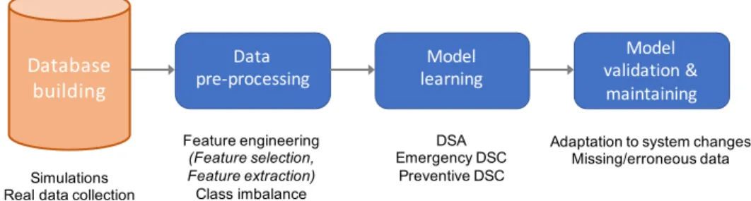
SECURE

ASECURE

INSECURE

Maximize economy and minimize the effect of uncertain contingencies

NORMAL

IN EXTREMIS

Protections Split Load shedding

Foreseen or unforeseen disturbances Preventive control Emergency control (corrective) EMERGENCY ALERT Resynchronization Load pickup Partial or total service interruption Overloads Undervoltages Underfrequency... Instabilities E,:I E, I Tradeoff of corrective control preventive vs RESTORATIVE :E, I :E,:I E, I PREVENTIVE STATE

SYSTEM NOT INTACT

E : equality constraints I: inequality constraints

Control and / or protective actions

Fig. 1. State transition diagram for security control (Adapted from [2])

(of electricity) to the system end-users. Reliability manage-ment concerns taking decisions to ensure that, in spite of uncertainties, the system reliability shall be suitable over some specified future time horizon.

With a long-term perspective (indicatively, 10-30 years in advance), the main decision is to define the additional infrastructure investments needed to keep the future system reliable enough. Next, in a mid-term context (typically 1-5 years ahead in time), the prevailing question is how to maintain the functionality of the existing system through repairs and/or replacements of its individual components. Last, but certainly not the least, short-term operation planning (a few months to a few hours ahead) and real-time operation jointly aim at deciding how to optimally deliver electricity from the producers to the end-users while enabling equipment maintenance and infrastructure building activities.

Various types of uncertainties and various spaces of can-didate decisions challenge all these complex and large-scale decision making problems. Better uncertainty modelling, en-hanced probabilistic and/or robust decision making frame-works, and more effective algorithms for optimal decision making under uncertainties are therefore main directions of R&D in electric power systems reliability management.

B. Adequacy & security

From a functional standpoint, power system reliability can be sub-divided into adequacy and security [3], respectively defined as,

Adequacy – the ability to supply with high enough probability the end-users at all times, taking into account outages of system components;

Security – the ability to withstand sudden disturbances such as electric short circuits or nonanticipated loss of system components without major service interruptions.

A reliable power system thus exhibits both (i) redundancy to adequately supply the load demand even when some of

its components remain unavailable, and (ii) plasticity to se-curelyride-through sudden, unanticipated disturbances and/or disconnections of some of its components.

Adequacy emphasises on the system dimensioning to ac-commodate the variability and stochasticity of the end-user demand, while also taking into account the (random) un-availabilities of system components. Typically, (in)adequacy is evaluated over a period of time, ranging from a few months to many years, and expressed by indicators such as loss of load probability or expected energy not supplied [3]. It may also be quantified in terms of the socio-economic impact of service interruptions to the system end-users, through indicators such as the expected cost of energy not supplied. Explicit adequacy criteria are commonly used in long-term planning applications adopted by many system operators [4].

Security complements adequacy by focusing on the opera-tion of the system while it undergoes state transiopera-tions initiated by unexpected exogenous disturbances and is canalised by various preventive or corrective control actions (cf. “The adaptive reliability control system” of T. Dy Liacco [5]). The diagram shown in Fig. 1, originally introduced in [2] based on a simpler version already given in [5], depicts the transitions among power system states from the security perspective. Security assessment aims at determining at which security level the system is currently residing, whereas security control aims at deciding control actions to move towards a more secure state. The vast domain of security (assessment and/or control) is further decomposed into dynamic and static security (assessment and/or control).

Dynamic security characterises the ability of the system to complete the transition from the pre-disturbance operating state to a post-disturbance stable equilibrium state. Here, three main physical phenomena are at (inter)play, giving rise to respective classes of (in)stability, namely rotor-angle, voltage and frequency (in)stabilities [6]. We refer the reader to the textbook of Kundur [7] for an explanation of the physical and mathematical modeling properties of these phenomena.

Rotor-angle stability concerns the equilibrium between the mechanical (input) and electromagnetic (output) torque of synchronous generators, keeping all machines of an intercon-nected power system rotating at a common angular speed. It is further classified into small-signal and transient rotor-angle stability, according to the magnitude of the studied distur-bances. Transient rotor-angle stability concerns the ability to sustain large disturbances such as short-circuits followed by the disconnection of one or more transmission lines, whereas small-signal stability concerns the ability to absorb stochastic variations of demand and generation. The physics of both concern relatively fast dynamics ranging over a few seconds following a disturbance.

Voltage stability refers to the ability of the power system to avoid an uncontrollable deterioration of the voltage level at its buses. At the extreme, voltage collapse is the situation wherein the system bus voltages reduce to unacceptably low levels. The behaviour of electrical loads and tap-changing voltage transformers restoring the consumed power after a disturbance is the main phenomenon potentially driving the system to voltage collapse. The dynamics of these phenomena

are typically slower than those concerning rotor-angle stability, and they may range over several minutes.

Frequency stability concerns the ability of the system to contain the frequency deviations caused by large mismatches between generation and demand resulting for example from the loss of large generators or fast variations of the load. Frequency stability is an issue of major concern under islanded operation, following some event that results in splitting the interconnected power system into disconnected under-/over-generated sub-parts. In systems with low electromechanical inertia, such as systems with predominantly photovoltaic and inverter-connected wind-power generation systems, frequency (in)stability is likely to become a major problem. While loss of synchronism typically takes at most a few seconds, frequency instability may take up to a few minutes to develop, and its study thus requires the modeling of slower processes such as boiler dynamics and load recovery mechanisms.

Finally, static security characterises the viability (typically over a period of 5 − 60 minutes) of the steady-state reached by the system following a contingency (i.e. a sudden line, transformer or generator outage). The main physical aspect of interest is compliance with the permanent capabilities of the system components (e.g. current carrying or electric isolation capabilities). Static Security Assessment (SSA) can be carried out by using a Power Flow (PF) solver to calculate a post-contingency state for each element of a set of contingencies. In current practice the so-called “N-1” contingency set is most often used: it is the set of disturbances corresponding to single-component trippings (“N” denotes the total number of such components). On the other hand, the Optimal Power Flow (OPF) problem may be solved in order to determine least cost decisions making a steady state viable.

C. Reliability assessment vs reliability control

Managing the aforementioned aspects to ensure the re-liable supply of electricity is in practice achieved through the functions of reliability assessment and reliability control. Reliability assessment concerns evaluating the security and adequacy metrics necessary to assess whether the system reliability level is acceptable with respect to a certain reliability criterion. It can be performed ex-ante to determine whether taking a certain candidate decision suffices to achieve the reliable operation of the system over a future horizon, or ex-postto evaluate the effect of already taken decisions over some past operational period. Reliability control concerns finding the decisions so as to ensure that the system will comply with a certain reliability criterion, and while optimising a socio-economic objective [8]. The formalisation of reliability assessment and control problems, as well as the challenges for tackling these, depend on the precise reliability management context of interest.

Starting from the shortest horizon, in the context of real-time operation, the salient feature is the lack of computational time to simulate the behaviour of the system in the time-domain, re-evaluate the static operability of the system vs credible contingencies and search for appropriate remedial actions. It is thus necessary to rely on security rules prepared off-line

to classify the system dynamic security, while monitoring its operation and its compliance with static security limits. Similarly, emergency controls need to be implemented as soon as possible to contain the unwanted deterioration of the system state before it escalates, and thus can only be triggered on the basis of pre-defined strategies. The challenge is therefore to design simple yet robust assessment rules and closed-loop control strategies, while also taking into account the reliability of protection, control and communications infrastructures.

In the short-term operation planning context, reliability management is further complicated by the need to take into account (i) the uncertainty on the potential pre-disturbance operating state of the system and the temporal evolution thereof, and, (ii) the future remedial actions to be implemented as per the respective real-time operation strategies. Analytical methods, such as time-domain simulations for dynamic secu-rity, power flow and optimal power flow for static security and adequacy are the primary tools for reliability assessment. The approach boils down to using such tools over a representative sample of potential operating conditions, to compute estimates of the respective metrics. The challenge is of course related to the size of the sample needed to reach acceptable accuracy. The Security Constrained Optimal Power Flow (SCOPF) is the fundamental statement expressing the operation planning reli-ability control problem, focusing mostly on static security [9]– [11]. Different variants of this problem are cast under different assumptions to fit specific operation planning questions (e.g. from the linear, so-called Direct Current or DC approxima-tions employed in market-based generation dispatching to the optimisation of preventive/corrective actions under the non-linear Alternating Current or AC power flow model). Further from the dimensionality issues associated with injection (i.e. load and generation) uncertainties, a key issue here is how to effectively integrate dynamic security limitations in the framework of such problem.

Taking the mid-term asset management perspective, the cen-tral question for reliability assessment concerns the criticality of a certain asset for the power system functionality, with emphasis on the adequacy and static security aspects. Answer-ing this question entails essentially simulatAnswer-ing the operation of the system with and without the asset in question, using again power flow and optimal power flow methods in a Monte Carlo style approach. Reliability control seeks to identify which assets to maintain and when to do so. Component-based reliability rules, triggering maintenance activities by age, condition, maintenance frequency etc. are useful in practice to answer the former question, taking into account the large number of system components. The problem of maintenance scheduling includes logistical considerations on top of the crit-icality of assets for the network functionality. Such logistical considerations reduce the (theoretically large) set of potential maintenance schedules in a calendar year, to a smaller subset of alternative moments per component in question. Still, the scheduling question implies a large-scale stochastic mixed-integer programming problem and the typical approach is to use heuristics for finding a suitable moment for each prioritised maintenance activity, while minimising the impact on reliable operation.

Finally, given the vast uncertainties in a long-term horizon, reliability management can only be achieved by a recursive ap-proach integrating assessment and control. The first step entails identifying the needs of the future power system, employing both adequacy/static security tools in Monte Carlo simulations as well as dynamic security consideration to frame potential future reliability problems. Exhaustive search is far from being an option here and the challenge is to combine micro-and macro- assumptions to generate manageable subsets of future operational conditions. Based on identified problems, expert knowledge as well as considerations on project timeline feasibility, public acceptability, etc. are employed to arrive at a small, manageable subset of potential solutions to the identified needs. These solutions then need to be re-assessed over a new set of realisations from the uncertainty models while the final choice requires detailed study of both the static and the dynamic behaviour of the resulting grid, as well as socio-economic analysis with a view on electricity markets and on the impact on the natural environment.

III. MACHINE LEARNING CONCEPTS

Machine learning exploits data gathered from observations or experiments on a system to automatically build models predicting or explaining the behaviour of the system, or decision rules to interact in an appropriate way with it. In this section we introduce the basic concepts of this field, to serve as the background for sections IV-VI, in the interest of readers outside the machine learning community. In particular, we introduce the different types of machine learning problems with a focus on supervised learning, feature selection and engineering, how to choose a method, and how to assess the accuracy of a model.

A. Different types of machine learning problems

To introduce the main types of machine learning problems, we will use the probabilistic/statistical formalisation and ter-minology and restrict to the so-called batch-mode setting. We refer the interested reader to more general textbooks for further information [12]–[14].

1) Supervised learning (SL): Given a sample {(xi_{, y}i_)}n i=1

of input-output pairs, a (batch-mode) supervised learning algo-rithm aims at automatically building a model ˆy(x) to compute approximations of outputs as a function of inputs.

The standard probabilistic formalisation of supervised learn-ing considers x ∈ X and y ∈ Y as two (vectors of) random variables drawn from some (joint) probability distribution Px,y

over X × Y , a real-valued loss function ` defined over Y × Y , and a hypothesis space H of “predictors” (i.e. functions from X to Y ), and measures the inaccuracy (named the expected loss, or average loss, or risk) of a predictor h ∈ H by

L(h) = E{`(y, h(x))} = Z

X×Y

`(y, h(x))dPx,y. (1)

Denoting by (X × Y )∗ the setS∞

n=1(X × Y )

n _{of all finite}

size samples, a (deterministic) supervised learning algorithm A can thus formally be stated as a mapping

A : (X × Y )∗→ H (2)

from (X × Y )∗ into a hypothesis space H. Statistical learning theory studies the properties of such algorithms, in particular how well they behave in terms of loss L when the sample size n increases [12].

Since SL is the most common type of machine learning problem treated in reliability management, we describe in more details the characteristics of SL in section III-B.

Methods: Methods like decision trees, neural networks, linear regression, nearest neighbor, support vector machines etc.belong to this category.

Power system example: A first example application is the assessment of system stability after the occurence of a disturbance [15]. In that case, the target output y typically can take two values, stable or unstable, and the inputs x could be real-time measurements of voltage at each bus and power flow in each branch of the system. The problem then amounts to building a model ˆy(x) that predicts, based on the measurements, if the system is stable or unstable.

2) Reinforcement learning (RL): Given a sample of n trajectories of a system {(xiτi, d i τi, r i τi, x i τi+1, . . . , d i τi+hi−1, r i τi+hi−1, x i τi+hi)} n i=1,

batch-modereinforcement learning aims at deriving an approx-imation of an optimal decision strategy ˆd∗(x, t) maximising system performance in terms of a cumulated index (named reward) over a certain horizon T , defined by

R =

T −1

X

t=0

γtrt, (3)

where γ ∈ (0, 1] is a discount factor. In this framework, xt

denotes the state of a dynamic system at time t, dt is the

control decision applied at time t, and rt is an instantaneous

reward signal [14].

From a theoretical point of view, reinforcement learning can be formalised within the stochastic dynamic programming framework. In particular, supposing that the system obeys to time invariant dynamics

xt+1= f (xt, dt, wt), (4)

where wtis a memoryless and time invariant random process

and obtains a bounded time invariant reward signal

rt= r(xt, dt, wt), (5)

over an infinite horizon (T → ∞), one can show that the two following (Bellman) equations define an optimal decision strategy Q(x, d) = E{r(x, d, w) + γ max d0 Q(f (x, d, w), d 0_{)}, (6)} d∗(x) = arg max d Q(x, d). (7)

Reinforcement learning can thus be tackled by developing algorithms to solve these equations approximately when the sole information available is provided by a sample of system trajectories. The theoretical questions that have been studied in this context concern the statement of conditions on the sampling process and on the learning algorithm ensuring convergence to an optimal policy in asymptotic conditions (i.e. when n → ∞).

Methods: Methods such as Q-learning, State-Action-Reward-State-Action (SARSA), and more recently Deep Q Network (DQN) belong to this category.

Power system example: A possible application of rein-forcement learning in power systems is emergency control, where an RL algorithm could take a sequence of actions dt

when the system is in an emergency state in order to come back to a normal state, as in [16]. Other examples can be found in [17].

3) Unsupervised learning (UL): Given a sample of obser-vations {zi}n

i=1 obtained from a certain sampling distribution

Pz over a space Z, the objective of unsupervised learning

is essentially to determine an approximation of the sampling distribution. In the most interesting case, Z is a product space Z1× · · · × Zp defined by p discrete or continuous random

variables, and the main objective of unsupervised learning is to identify the relations among these latter, such as (conditional) independence relations or colinearity relations, as well as the parameters of their distributions.

Methods: Earlier work in this field concerned clustering (for instance with the k-means algorithm), Principal Compo-nent Analysis(PCA) and hidden Markov models. More recent research topics, still very active today, concern independent component analysis as well as the very rich field of graphical probabilistic models, such as Bayesian belief networks [13].

Power system example: In the context of powers systems reliability, unsupervised learning can be used for segmenting automatically large scale power grids into coherent zones to ease the management of the grid for control room operators [18].

4) Semi-supervised learning: Semi-supervised learning concerns a situation where the dataset is composed of a labelled sample {(xi, yi)}n_i=1 drawn from a joint distribution Px,y and a second (unlabelled) sample {(xj)}n

0

j=1drawn from

the corresponding marginal distribution Px. Semi-supervised

learning algorithms aim at exploiting both samples together to find a predictor h that is hopefully more accurate than what could be produced by a supervised learning algorithm using only the labelled sample.

These types of methods are useful when it is relatively ‘easy’ to collect unlabelled data but relatively ‘difficult’ to obtain labelled data.

Methods: Methods based on self-training, tri-training and other algorithms such as semi-supervised support vector machines belong to this category.

Power system example: In the context of dynamic secu-rity assessment, one could use time-consuming simulations to label as stable or unstable only a part of a database, and then use semi-supervised learning to exploit the whole database in order to build a classifier, as in [19].

B. Characteristics of supervised learning algorithms

In supervised learning a first main distinction concerns the nature of the output space. When Y is a finite set of ‘class labels’ one talks about classification problems (e.g. stable vs unstable), while when Y is embedded in the set of real num-bers (respectively in a finite dimensional euclidean space) one

talks about regression (respectively multiple-regression) prob-lems (e.g. stability margin). But, beyond these two standard types of supervised learning problems, there are many other ones, as many as one can imagine output spaces structured in some meaningful way.

Once an output space Y is defined, one can further refine the nature of the problem by defining a particular loss function `(y, y0) over Y × Y . For example, for classification problems one often uses the so-called 0/1-loss, which is defined by `(y, y0) = 1(y 6= y0) and counts the number of misclassifi-cations, whereas for regression problems one often uses the square-loss (y − y0)2_{. Once the loss function ` is defined, it}

means that one targets the so-called “Bayes” model, which is defined in a point-wise way by

hB(x) = arg min y0_∈Y

Z

Y

`(y, y0)dPy|x, (8)

and is among all functions h of x the one minimising the average loss L(h), defined as in (1). For example, in the case of regression problems and with the square-loss, hB(x) is

identical to the conditional expectation of y given x, whereas using the absolute loss |y − y0| would instead yield the conditional median.

The next step in defining a supervised learning algorithm consists of choosing a hypothesis space of functions H. As far as loss minimisation is concerned, this space should ideally contain the (problem-specific) Bayes model or at least models sufficiently close to it in terms of the chosen loss function.

Given a choice of H, the empirical risk minimisation prin-ciple then reduces supervised learning to solving the following minimisation problem:

A({(xi, yi)}n_i=1) = arg min

h0_∈H

n

X

i=1

`(h0(xi), yi). (9) One can show that if H is ‘sufficiently’ small, it produces models whose loss L converges towards minh∈HL(h), when

the sample size n increases, and that it converges faster if H is of smaller ‘size’. As far as accuracy is concerned, the SL algorithm should thus use an as small as possible hypothesis space containing good enough approximations of hB.

Nevertheless, in addition to accuracy, computational com-plexity of learning algorithms is often a concern. Indeed, solving an empirical loss minimisation problem may require huge computational resources if the hypothesis space is very complex and the sample size n is very large.

Finally, beyond making ‘low loss’ predictions, the goal of a machine learning application is often to help human experts to understand the main features of the problem at hand. Therefore, interpretability of the output of the machine learning algorithm is another often highly desired feature. C. Feature selection and feature engineering

When considering a particular application of machine learn-ing, the raw datasets that are available are typically recorded values of a large number of low-level individual variables zj, some of which could be either inputs xj, outputs yk, or

decisions dlof some supervised and/or reinforcement learning

Often, it is suspected that some (or even a majority) of these variables are actually irrelevant for the resolution of some particular prediction or optimal control task. In other applications, one would like to find a minimal subset of input variables to be used by a supervised or reinforcement learning method, so as to facilitate the practical application of the resulting predictor or control policy without sacrificing too much in terms of accuracy.

Thus, the machine learning field has developed various methods for selecting “optimal” subsets of input variables (feature selection) and for computing useful functions of the original variables (feature extraction), based on the informa-tion provided in a dataset [20].

D. Practical choice of a supervised learning method

The different supervised learning algorithms available today (see [12], [13]), yield different compromizes between inter-pretability, computational efficiency, and accuracy.

The choice of the most suitable algorithm is thus highly application dependent, for several reasons: (i) the application determines which one of these three criteria is the most important one in practice; (ii) the application determines the data-generating mechanism and loss function, hence the Bayes model hB and thus how well different hypothesis spaces allow

to approximate this ideal target predictor; (iii) the application domain conditions the size of the possibly available datasets, impacting both accuracy and computational efficiency of most algorithms, but in different ways.

This situation means that, typically, the one who is faced with a particular application will try out a (more or less large) subset of machine learning algorithms, analyse their behaviour and results, and select the one which seems to fit in the best way the need of the considered application. This “trial and error” type of approach is the price to pay for the very broad scope of machine learning applications.

E. Overfitting and honest model assessment

Because the empirical risk minimisation chooses models to minimise the average loss over the learning sample, this empirical risk is in practice strongly biased in an optimistic way. It means that even if the selected predictor works very well on the learning sample, there is no guarantee that it will work well also on an independent test sample drawn from the same distribution.

In order to assess the accuracy in an honest way, various approaches have been developed and studied, such as the “hold-out” method which keeps part of the data as a test sample and uses only the rest of them to apply the learning algorithm, or the k-fold cross-validation approach, which uses the data in a more effective way at the price of higher computational requirements [12].

Often, the cross-validation approach is also used in order to select among several algorithms the one more suited to a par-ticular dataset, or to adapt some algorithm’s “meta-parameters” (e.g. number of hidden neurons, training epochs, strength of weight decay penalisation), or even to help identifying a subset of relevant input features. If this is the case, then a nested

model assessment approach is needed in order to honestly assess the accuracy of the finally produced predictor [12].

IV. PUBLICATION STATISTICS SINCE2000

In this section, we survey recent contributions to the field of machine learning for electric power systems reliability. We found (via Google Scholar and Scopus)1 366 papers in this subject field that were published between January 2000 and October 2019; their yearly counts are shown in Figure 2, which clearly shows a strong growth over the last 5 years.

2000 2001 2002 2003 2004 2005 2006 2007 2008 2009 2010 2011 2012 2013 2014 2015 2016 2017 2018 2019 Year 0 10 20 30 40 50 60

Number of papers published

6 611714 13 15 12 12 15 18 11 12 19 1014 30 39 57 45

Fig. 2. Yearly number of published papers we found on the topic of machine learning application to electric power systems reliability

DSA DSC SSA SSC Others

0 50 100 150 200 Number of papers 203 50 66 31 16

Fig. 3. Number of ML papers (01/2000 - 10/2019) per reliability management problem (DSA = dynamic security assessment, DSC = dynamic security control, SSA = static security assessment, SSC = static security control)

SL UL RL 0 50 100 150 200 250 300 350 Number of papers 323 25 20

Fig. 4. Number of papers per ML protocol (01/2000 - 10/2019)

Figure 3 shows the statistics of these papers in terms of the different types of reliability management problems they address. We observe that more than 50% of them address the problem of dynamic security assessment. On the other hand,

1_{We used the following keywords to gather these papers: i. power system,}

reliability, security, stability, learning; ii. power system, reliability, security, stability, assessment, control, learning; iii. power system, reliability, security, stability, assessment, control, learning, neural network, ANN, support vector, SVM, nearest neighbours, decision tree, random forest. The retrieved papers were analysed one by one to eliminate irrelevant ones from the statistics.

we have observed a recent growth of the number of papers applying machine learning to power flow and optimal power flow computations (which are classified into the SSA and SSC categories respectively).

Another interesting analysis is the type of machine learning protocol exploited in our set of papers. Figure 4 shows the number of papers using supervised learning, unsupervised learning and reinforcement learning. It is clear that supervised learning is by far the most popular type of machine learning protocol used in these reliability management applications.

In the following two sections, we present in more details how the different reliability management problems are ad-dressed in the literature with a machine learning approach. We first present papers exploiting machine learning for dynamic security assessment, as well as (dynamic) emergency and preventive control, since they constitute the largest part of our survey. Then we present how machine learning was applied for static security assessment and control, and to speed up optimal power flow and power flow computations. We focus this literature survey on the last 5 years. Table I presents an overview of the works discussed in the next two sections, classified in terms of the respective power system reliability management application (i.e. transient, voltage, frequency or small-signal stability, dynamic and static security).

V. WORKS ONMLFORDSA & DSCSINCE2015

Dynamic security is a particularly suitable application for machine learning, given the need for fast assessment and control and the computational burden inherent to classical approaches such as time-domain simulations. Figure 5 shows the four steps generally followed to exploit machine learning in this context. We discuss them one-by-one hereafter. A. Database building

The first step to apply machine learning for security assess-ment and control is the database building. In most papers, due to lack of historical data availability, simulations are used to generate a security database. Another advantage of simulation is that it allows to sample operating points defining well the security boundary, which is typically not the case with historical data, for which most operating points are stable [21]. The database generation is then usually done offline, given the extensive simulation cost to build it, while the application of the resulting model trained on the dataset can be done offline or online, depending on the application and the context.

TABLE I

MAIN SECURITY PROBLEMS ADDRESSED WITH A MACHINE LEARNING APPROACH AND CORRESPONDING REFERENCES

Security problems addressed References

Transient stability [15], [16], [19], [22], [27]–[29], [32], [34], [35], [37], [38], [41], [43], [45], [47], [49]–[52], [54]–[56], [63], [64], [67]–[73], [75], [76], [81]–[83], [85]–[88], [90], [92], [93], [98], [102], [105], [107], [113], [115]–[117] Voltage stability [26], [30], [39], [40], [42], [44], [46], [48], [53], [60], [65], [66], [78], [79], [89], [91], [97], [100], [103], [108]–[110], [114], [123] Small-signal stability [21], [22], [61], [62], [74], [120], [121] Frequency stability [80], [84], [104], [106], [112] Dynamic security [25], [31], [33], [36], [57]–[59], [77], [94], [95], [99], [101], [118], [119], [122] Static security [18], [23], [24], [74], [96], [111], [120], [121], [124]–[175]

In order to generate a database based on simulations, the first step is to generate representative operating states of the system. The main uncertainties in power systems relate to load patterns, topology configuration and generation. It is impossible to sample all operating conditions and therefore Monte-Carlo simulations are used in most papers, but other techniques to sample from a multi-dimensional distribution are possible, such as the latin hypercube sampling [22].

In DSA and DSC applications, the input-features of the database often come from Phasor Measurement Units (PMU), which are devices allowing to monitor the power system state in real-time. They measure synchronously voltage phasors at buses where they are located and current phasors in the branches connected to these buses.

The target output of the database depends on the task. Most studies build classifiers to predict the stability status of the system, considering either transient, small-signal, voltage or frequency stability. Others are more interested in quantifying the distance to instability, by exploiting regressors to predict for instance the security margin, the voltage stability index, the so-called Critical Clearing Time (CCT), i.e. the maximum time available to clear a disturbance before the system becomes unstable, etc. Finally, for control purposes, some predict directly which decisions, such as generation re-dispatch, to

Model learning Database building Data pre-processing Model validation & maintaining Simulations Real data collection

Feature engineering (Feature selection, Feature extraction) Class imbalance DSA Emergency DSC Preventive DSC

Adaptation to system changes Missing/erroneous data

apply. These outputs are usually obtained with time-domain simulations of the power system.

The quality and representativity of the database has a major impact on the effectiveness of the ML approach. For instance, for a database based on simulation, if the representation of the problem is too simple, this could lead to a learnt model with very good performance on data generated with the same distribution as the database but bad performance when it is used in practice, in a real situation. Furthermore, the input variables must allow one to discriminate well the target output(s). If it is not the case, the problem may be hard to learn and one may overfit noise, which could lead to difficulties to obtain an efficient model. The database must also be large enough for the model to be able to capture all the subtleties of the studied problem, in order to obtain high generalisation performances. Another important aspect for the person exploiting the database is to know the hypotheses used to generate it, if this is a database based on simulations, and to know the data collection process, if if it is based on real-life data. In general, when the quality and/or representativity of the database is insufficient, the learnt models cannot be used to perform security assessment and/or control in practice.

Recently, given the importance of the database genera-tion step, papers focusing mainly on building more effective databases for machine learning-based security assessment and control were published [21], [23], [24]. In [23], the authors propose an approach using Vine-Copulas to generate more representative states of power systems. They show on a test-case that the security classifier built with this approach is superior to the one build with data obtained from a classical approach. Thams et al. exploit in [21] convex relaxation techniques and complex network theory to discard large parts of the input space and thus focus on the regions closer to the security boundary. In order to build a database representing well the security boundary, they use a ‘Directed Walks’ algo-rithm to identify the security boundary. Finally, [24] proposes a method to generate datasets to characterise the security boundary which cover equally the secure and insecure regions. In particular, they introduce infeasibility certificates based on separating hyperplanes to identify, for large portions of the input space, the infeasible region.

Furthermore, to help dealing with a massive amount of data, in [25], the authors propose a distributed computing platform for data sampling, feature selection, knowledge discovery and online security analysis.

B. Data pre-processing

Once a dataset is built, the data can be processed before being fed to a learning algorithm. This step may in some cases be mandatory. Processing the data can improve the quality of the predictions of learning algorithms, increase training speed and transform data in more meaningful representation to facilitate model training. In this section, we distinguish feature engineering and class imbalance management. Table II provides an overview of the main data pre-processing methods used for DSA and DSC discussed below.

TABLE II

MAIN DATA PRE-PROCESSING METHODS USED FORDSA & DSCOVER THE LAST FIVE YEARS AND CORRESPONDING REFERENCES

Methods References Feature engineering Feature selection Filter methods [22], [26]–[36] Wrapper methods [34], [35], [37] Genetic algorithms [38], [39] Tree-based algorithms [40]–[43] Feature extraction

PCA and variants [44]–[46]

Fisher’s linear

discriminant [47]

Shapelets for time

series [48] Deep learning auto-encoders [49]–[52] Class imbalance Oversampling [24], [53], [54] Cost-sensitive learning [53], [55] Ensemble methods [41], [45], [56], [57]

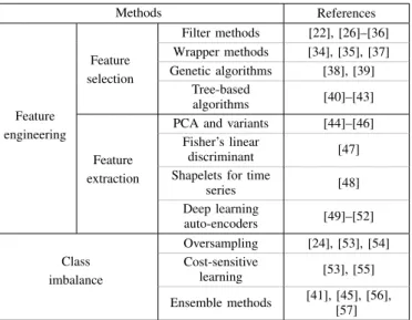
1) Feature engineering: Given the large number of features necessary to fully describe the state of a power system and the need for fast algorithms, feature selection techniques are proposed in many papers. Too many features can lead to exces-sive training time and, if many features are not relevant, could decrease the performance of the learnt model. In the machine learning literature, several techniques have been proposed to reduce the number of features. In power systems applications, the ‘Relief’ method, which is is a filter-based method, has been used alone [22], [26], or combined with a PCA to reduce even more the number of features [27], [28]. Variants of this method such as ‘Relief-F’ have also been used [29]–[33], mostly to improve the predictions of randomised learning algorithms such as extreme learning machines.

Combining both filter and wrapper methods for feature selection, Zhou et al. [34] use the improved ‘Relief-Wrapper’ algorithm to select a subset of features and in [35], the authors propose a hybrid filter-wrapper feature selection algorithm using the ‘Relief-F’ method to find top weighted features and then the Sequential Floating Forward Selection method to select the most relevant set. In [37] a backward feature selection approach is used, on the other hand.

Genetic Algorithms (GAs) can also be used to select fea-tures. In [38], the authors use Particle Swarm Optimization (PSO) based feature selection. Packets of features are drawn randomly with PSO and the selected packet is the one max-imising the mean of the standard deviations of the packet. In [39], the authors first apply a mutual information criterion to remove less significant features from the dataset and then use a multi-objective biogeography-based optimisation program to keep the most relevant ones.

In [36], the authors use the symmetrical uncertainty to reduce the number of features and improve the performance of the algorithm. It consists in computing correlation between pairs of features based on entropy and mutual information, to keep relevant features and remove redundancy.

learning algorithms. These algorithms allow to evaluate the importance of each feature for predicting the target output. Feature importances are by-products of the tree-based algo-rithm and can be used to identify the most important features, such as in [40]–[43]. This can also give insight about the power system dynamic security assessment problem under consideration.

Feature selection algorithms allow to select the most rel-evant features. Another field of feature engineering is the feature extraction field. It consists in transforming the data to represent it in a more meaningful way, facilitating the learning. Generally, it also reduces the dimensionality of data. PCA and its variants are often used as a feature extraction tool [44]– [46], as well as Fisher’s linear discriminant [47] and shapelets for time series [48] but recently, an approach based on deep learning auto-encoders was proposed [49]–[52].

Furthermore, feature selection can help to find the most useful PMUs in a network, e.g. the least number and best locations of PMUs for a given DSA application [37], [42].

2) Class imbalance: In most databases, the proportion of stable observations is much larger than the proportion of unstable ones. This is due to the high reliability of power systems. However, this imbalance between classes can degrade the quality of the learnt models, that could be biased toward the majority class. The problem is particularly important, given that unstable events must be detected to guarantee the relia-bility of the system. To overcome this issue, several solutions have been proposed in the literature, such as oversampling the minority class [24], [53], [54], undersampling the majority class, exploiting a cost-sensitive learning [53], [55] and using ensemble methods [41], [45], [56], [57].

Oversampling is usually preferred to undersampling, to avoid loss of information. The Synthetic Minority Oversam-pling Technique (SMOTE) adds new observations of the minority class by interpolating linearly data points between adjacent observations of the minority class. A variant of the SMOTE technique is used in [53], combined with cost-sensitive learning to compensate for class imbalance. Cost-sensitive learning consists in using different costs for different classes during learning, in order to, for instance, avoid as much as possible misclassifying unstable samples. Using another ap-proach, suitable because of their data representation as images, Hou et al. artificially increase the number of samples of the minority class by using a multi-window sliding recognition method [54]. The database generation method proposed by Venzke et al. in [24] allows to generate balanced dataset between secure and insecure labels.

Ensemble methods can also help for class imbalance prob-lems. For instance, in [56] the authors exploit the diverse extreme learning machine algorithm to determine transient sta-bility. They show that adding diversity can improve accuracy in case of the class imbalance problem. Another example is the use of bagging and, instead of sampling uniformly in the training set, sampling to obtain balanced subsets of training set [45]. Finally, it is possible to use an Adaboost ensemble method, which adapts itself to class imbalance [57], or a ‘Weighted Random Forest’, that gives more weight to the unstable observations when learning [41].

Reference [55] uses an ad hoc loss to avoid instability detection while [53] uses distinct costs for stable and unstable observations while learning, in order to minimise the misclas-sification of unstable samples.

C. Learning a model

Many learning algorithms have been tested to build models for DSA & DSC. Most of the time, training is done of-fline but the model is sometimes updated online. Recently, given the success of deep (neural networks) learning, several papers have proposed to use this technique. However, other learning algorithms such as decision trees and Support Vector Machines (SVMs) are still exploited. Ensemble methods are also proposed in the literature to improve performances. In this section, we present how ML algorithms are exploited for dynamic security by considering first security assessment, then emergency control and finally preventive control.

1) Security assessment : DSA applications are particularly suitable to apply machine learning techniques and many papers exploiting ML to improve DSA were found over the last five years. Table III provides an overview of the main machine learning algorithms used for DSA. The acronyms that appear in the table are defined in the discussion below.

Since many learning algorithms exist, all with their advan-tages and disadvanadvan-tages, comparing several algorithms with your dataset is the best way to know which algorithm is more suitable for your application. In [28], a decision tree model is compared to SVMs and neural networks for transient sta-bility assessment. The same algorithms are compared in [58], but this time considering also the random forest algorithm. Reference [85] compares decision trees, SVMs, core vector machines and naive Bayes models while [91] compares several ensemble methods (XGBoost, Bagging, Random Forest, and AdaBoost) with Naive Bayes, k Nearest Neighbor (kNN) and decision trees, this time for voltage stability assessment. In [59], the authors propose an automated multi-model approach for online security assessment. In [60], several learning algo-rithms such as random forests, Kohonen networks and hybrid neural networks were tested to predict the security status, considering several labels such as normal, alarm, serious alarm and emergency. Note that, depending on the application, the most suitable algorithms may change.

TABLE III

SUPERVISED LEARNING ALGORITHMS USED FORDSAIN THE LAST FIVE YEARS AND CORRESPONDING REFERENCES

Algorithms References Neural Networks FFNN [22], [28], [58]–[69] CNN [49], [54], [55], [70]–[74] ELM [19], [29]–[33], [35], [56], [59], [75]–[80] RNN [37], [81]–[84]

Support Vector Machines (SVM) [15], [28], [39], [50], [51],

[57]–[59], [85]–[90] Tree-based methods Decision trees [28], [36], [42], [44], [48], [58], [59], [85], [91]–[96] Ensemble [27], [40], [41], [43], [58]–[60], [91], [97]–[101] k Nearest Neighbor (kNN) [45], [91]

Recently, due to the success of deep neural networks in other applications, many researchers tackled the dynamic security assessment problem with such an approach. Classical Feed-Forward Neural Networks (FFNNs) are used as classifiers to predict the small-signal stability [61], oscillatory stability [62] or transient stability [63]; or as regressors to predict the CCT or damping ratio [22], the CCT and final value of rotor angle after a fault [64], the load stability margin [65] or a voltage stability index [66]. In [67], a MapReduce algorithm is used to parallelise the learning of several networks and predict both stability status and the transient stability index. In [68], when the prediction is not credible, time-domain simulations are used to improve the efficiency and in [69], in the context of pre-fault assessment, contingencies are first clustered and then a multi-label neural network is learnt per cluster, to predict the stability status after the occurrence of each contingency in the cluster.

Reference [46] proposes to use deep belief neural networks for voltage stability and another ensemble of neural networks with random weights to predict first if there will be a voltage collapse and then, if no voltage collapse is detected, the transient voltage severity index [26]. Another neural network approach is the Extreme Learning Machine (ELM) algorithm. It is fast to train, and thus can be easily updated during operation. In the literature, ensembles of ELMs are used mostly for stability classification [19], [29], [32], [35], [56], [75], [76], or combined with random vector functional links [31], [33], [77]. It was also used for regression, to predict load stability margins [78], the fault-induced voltage recovery [30], [79], and maximum frequency deviation and time [80].

Convolutional Neural Networks (CNNs) have also been used, in particular for transient stability assessment [49], [54], [55], [70]–[73]. Reference [74] proposes to represent the power system state as a (3-channel) image to take advantage of the convolutional neural network algorithm for small-signal stability. In [70], a twin convolutional SVM network is used while in [72] a hierarchical self-adaptive method, with one CNN per type of features, determines the stability of the system. In [73], a cascade of CNNs works with time-domain simulation to improve efficiency for pre-fault assessment. Time domain simulations are performed one cycle at a time and are used as inputs of the CNN. If the prediction of the CNN is credible, time-domain simulations are stopped.

Recently, Recurrent Neural Networks (RNNs) were also proposed, because of their ability to consider temporal cor-relations, either with Long Short-Term Memory (LSTM) units [37], [81], [82] or Gated Recurrent Units (GRU) [83], [84].

More classical algorithms are however still exploited in the literature. For instance, SVM methods are used for transient stability [50], [51], [86]–[88] or voltage stability [39], [89]. SVMs are easier to train than neural network models and they can be used to predict the stability status of the power system (stable or unstable) or a voltage stability margin index [89]. The parameters of the SVM can be optimised with a grid search algorithm or particle swarm optimisation [88], [89]. In order to increase the accuracy of the assessment, in [87], two SVM models are used, an aggressive and a conservative one. This allows to predict a third class, called the grey region,

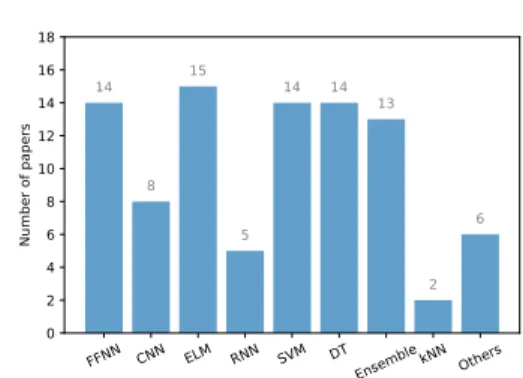
FFNN CNN ELM RNN SVM DT_{EnsemblekNN Others} 0 2 4 6 8 10 12 14 16 18 Number of papers 14 8 15 5 14 14 13 2 6

Fig. 6. Number of papers addressing power system dynamic security

assessment problems per machine learning algorithms

when both models disagree, to indicate when the assessment is uncertain. Ensembles of SVMs [57], [90] or variants of the SVM such as core vector machines [15] have also been proposed to increase the accuracy of the classification.

Tree-based methods are still popular in the power system literature. A huge advantage of them is their interpretability, which is important in reliability management. Single Decision Trees (DTs) are used to predict the stability status of the system [36], [42], [44], [48], [92]–[94]. In [94], the authors ex-plore a trade-off between predictive accuracy and interpretabil-ity. To improve accuracy, ensembles of decision trees such as Adaboost [27], [97], XGboost [43] and Random Forests [40], [41], [98]–[101] are proposed. In [101], uncertain predictions are checked with time-domain simulations. In the European project iTesla, decision trees are used for online security assessment. The platform developed within this project for online static and dynamic security assessment is presented in [95], [96].

The simple kNN algorithm is used in [45] with bagging to predict transient stability. Logistic regression, after a stacked denoising auto-encoder is used in [52] to predict post-fault stability status. Less common approaches have also been proposed, such as unsupervised learning with PCA [102] and semi-supervised learning when few observations are labelled [19]. In the latter, the ‘Tri-training’ algorithm is used, which consists in training three models with a small subset of labelled data and then adding an unlabelled sample to the training set of a classifier only if the two other classifiers agree.

Figure 6 summarises the number of papers per learning algorithm for DSA. One can notice that neural network algorithms have been very popular in the last five years.

2) Emergency control: Instead of predicting the stability state of the system, data-driven models can be used to choose an emergency control decision, or to give insight about the best corrective control actions for the actual situation. Table IV provides an overview of the publications about dynamic security emergency control according to the main machine learning approach used.

Reinforcement learning [16], [103], [104] or adaptive dy-namic programming [105], [106] are used to improve voltage, frequency or transient stability. Supervised learning techniques can also be used. For instance, in [47], the authors train a decision tree classifier to evaluate transient stability and thanks to the Fisher linear discriminant, they evaluate the sensitivity of each generator and load to stability and then

TABLE IV

MLPROTOCOLS ANDSLALGORITHMS USED FOR DYNAMIC SECURITY EMERGENCY CONTROL OVER THE LAST FIVE YEARS

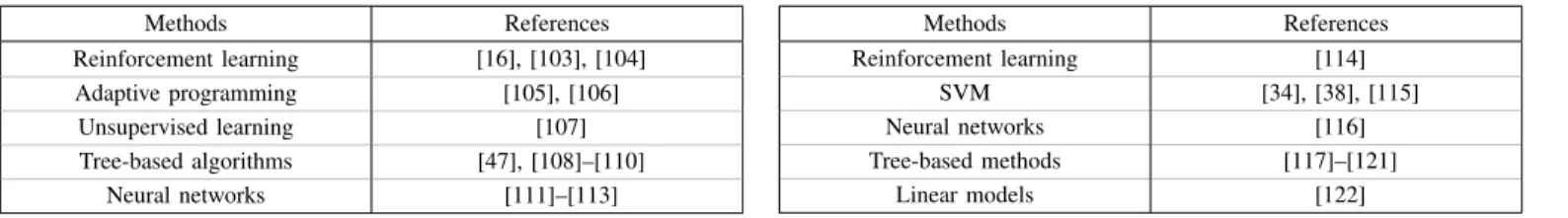
Methods References Reinforcement learning [16], [103], [104] Adaptive programming [105], [106] Unsupervised learning [107] Tree-based algorithms [47], [108]–[110] Neural networks [111]–[113]

define emergency control actions accordingly. In [111], the authors use a neural network to assess the generators that need to be re-dispatched and the loads that need to be shed.

In [107], patterns of unstable dynamic behaviour in the dataset are identified with an unsupervised learning technique and then a classifier is used to determine in which pattern the actual situation falls. This indicates which generators may lose synchronism to help for emergency control decisions.

In [108], an ensemble of decision trees is used to assess and control voltage stability. There is one decision tree per possible combination of control action status (1 or 0, depending if they are used or not), indicating which control combinations lead to a secure system. The control actions combination chosen is the one leading to a secure action with a minimum number of control devices used. This approach is also used in [109], but there is first identification of voltage control areas, to reduce control candidates.

In [112], the authors propose to control a hybrid energy storage system for load-frequency control. They design an adaptive control based on a neural network, the design of which being facilitated by a Hammerstein-type neural network to identify the storage system. In [110], the authors use a proximity driven streaming random forest algorithm with L-index as indices for voltage stability. The algorithm can determine corrective and/or preventive control actions, such as additional reactive power injections, and localise critical nodes, where the system is close to a stability loss.

In the context of transient stability, in [113] a neural network is used to estimate the gain for a static synchronous compensator auxiliary controller, that needs to be adjusted according to the system operation point to obtain the desired CCT. The gain computation is heavy and thus a neural network model is proposed to reduce the computational burden.

3) Preventive control: Several approaches have been pro-posed in the literature for preventive control regarding dynamic security. Table V provides an overview of the publications about dynamic security preventive control according to the main machine learning approach used.

The first approach consists in using machine learning to predict the preventive control scheme. For instance, in [114], the authors propose to use multi-objective reinforcement learn-ing for short-term voltage stability, in order to minimise both voltage deviation and control action cost.

The second approach consists in identifying candidate con-trol actions for preventive concon-trol. In [115], the authors pro-pose a preventive control scheme by rescheduling generating units. First, they assess the transient stability of the system

TABLE V

MLPROTOCOLS ANDSLALGORITHMS USED FOR DYNAMIC SECURITY PREVENTIVE CONTROL OVER THE LAST FIVE YEARS

Methods References Reinforcement learning [114] SVM [34], [38], [115] Neural networks [116] Tree-based methods [117]–[121] Linear models [122]

with a hybrid method based on a SVM model and time-domain simulation. Then, if the system is unstable, they compute from the SVM model the sensitivity of each generator to a transient stability assessment index (derived from the SVM model) to rank the generators and select the ones that are more effective for improving the stability. In [38] the authors exploit SVMs for determining the coherency of generating machines in the context of transient stability. The purpose is to rank generators according to their vulnerability, based on a transient stability index, to facilitate preventive control (rescheduling of gener-ation). Finally, in [32], the authors use the Relief-F feature selection method to identify critical generators modifying the security status of the operating condition. These generators are then considered as candidate control variables for preventive control. A bit different, but still to help preventive control, Mokhayeri et al. propose a method based on decision trees for detecting the apparition of islands [117].

Another main approach, quite recent, consists in building models of dynamic security assessment and then extracting security rules from these models that can be embedded in op-timisation problems, to define control actions considering dy-namic security. Indeed, classifiers built with machine learning contain knowledge about stable and unstable regions. Cremer et al. exploit decision trees to embed the rules determining the output of the classifier in a decision-making problem (i.e. an OPF) [118]. This allows to compute control decisions consid-ering the stability boundary. In their paper, the authors present the challenges of this approach, which are the computational complexity to build the database and the accuracy of the such sample-derived rules. This approach is further developed in [119], where learnt condition-specific safety margins are proposed to be incorporated in a decision-making program. These margins allow, according to the authors, to improve the risk/cost balance. An ensemble of decision trees (Adaboost) is used to perform probabilistic security control.

In [120], the authors propose to build with machine learning line flow constraints to be incorporated in a market clearing program (under the form of a SCOPF) to improve both small-signal stability and steady-state security. They use a decision tree-based classifier to extract knowledge. The decision trees rules consist in conditional line transfer limits, that can be embedded in the SCOPF in order for the operator to take decisions already in line with the small-signal stability margin. An extension of this work to solve an AC-SCOPF instead of a DC-SCOPF is proposed in [121], while still incorporating N-1 security and small-signal stability with decision tree-learnt rules. In [116], the authors are solving an OPF considering

transient stability constraints. An artificial neural network approximating the CCT of a fault is embedded in the OPF formulation. This guarantees that the preventive decisions will be such that the CCT of all considered faults is greater than a defined minimum value. A bit different but still embedding a machine learnt model in an optimisation program, the authors of [34] build a two-stage SVM model to determine the transient stability region that is embedded in a decision-making program to determine preventive control actions. The final transient stability-constrained OPF being non linear and non convex, the authors propose to solve it with particle swarm optimisation. Finally, in [122], the authors propose to automatically learn operating rules for a stability constrained system.

D. Validating and maintaining a machine learnt model In this section, we present first how researchers in relia-bility management proposed to deal with the frequent system changes in a power system and then what can be done when data is missing or erroneous.

1) Dealing with system changes: System changes such as topology changes are common in power systems but they can impact the quality of prediction of the machine learnt models. To overcome this issue, several papers propose to regularly retrain or update the model with new data acqui-sition. Regarding neural network models, in [65], the model is updated with misclassified samples when a certain number of errors occurred. Online sequential ELM models were also proposed, as in [32], [80], because they are fast to train and can be updated regularly. Another approach is to use a recurrent neural network. In [83], an online monitoring system, consisting in a stacked GRU based recurrent neural network, is shown to be able to adapt to topology change. Concerning tree-based methods, Yang et al. update decision trees in real-time using an online boosting method [108], while [97] presents a very fast decision tree system based on Hoeffding trees to quickly update online an Adaboost ensemble of decision trees. Furthermore, Tomin et al. propose the proximity driven streaming random forest algorithm that can independently and adaptively change the model [110].

Another solution proposed in the literature is active learning [71], [123]. For instance, in [123], the authors propose an active learning solution that consists in updating the model with real samples when the model prediction is not consistent with the actual system condition. More specifically, they train and update the model with data for which the prediction contradicts with the actual stability state of the system.

2) Missing or erroneous data: During online assessment or control, when exploiting PMU data, many events can occur such as PMU malfunctioning, time delays, communication loss, noise in the measurements and loss of data packets. Therefore, it is important to develop models able to deal with these missing data or erroneous measures. When erroneous measure are outliers, they can be detected, for example by using the Z-score algorithm [65]. Concerning missing data or detected erroneous measures, it is possible to estimate their values, either by interpolation techniques such as polynomial

curve fitting technique [65] or by using machine learning techniques such as an ensemble of extreme learning machines and random vector functional links [33] or the emerging deep learning technique called Generative Adversarial Networks (GAN) [77]. Instead of replacing missing data with estima-tions, some authors try to build a model robust to incomplete measurements by extending the training database with samples containing incomplete measurements [86].

VI. RECENT WORKS INSSA & SSC

The methodology to exploit machine learning for static security assessment and control is similar to the one used for dynamic security, although the input variables and target outputs vary in function of the application. Therefore, we directly present how ML is applied to solve the different static security assessment and control problems. We organised this section considering the power system tool that is considered to be replaced or enhanced with machine learning techniques. In particular, we consider power flow computation, optimal power flow solving, and unit commitment optimisation. A. Prediction of power flows

Table VI sets out the main target outputs of the ML methods used in the context of static security assessment, to replace or enhance power flow computations, the exploited learning algorithms, as well as their corresponding references.

Some papers studied the possibility to replace the power flow computation by a proxy, for a faster static security assessment. For instance, [124] uses a deep neural network to estimate power flows very quickly. The authors propose to exploit it to help operators in the control room to choose remedial actions such as network topology modification after a contingency. Improving their previous work, they introduced guided dropout to enable the estimation of flows for a range of power system topologies [125]. The guided dropout method uses some neurons that are only activated if the corresponding

TABLE VI

MAINMLAPPROACHES FOR POWER FLOWS PROBLEMS OVER THE LAST FIVE YEARS AND CORRESPONDING REFERENCES

Predicted quantities Algorithms References

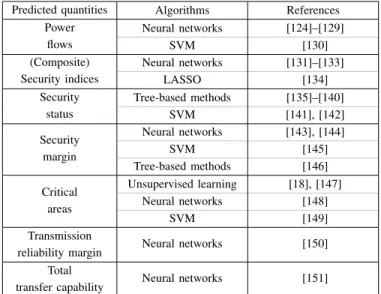
Power flows Neural networks [124]–[129] SVM [130] (Composite) Security indices Neural networks [131]–[133] LASSO [134] Security status Tree-based methods [135]–[140] SVM [141], [142] Security margin Neural networks [143], [144] SVM [145] Tree-based methods [146] Critical areas Unsupervised learning [18], [147] Neural networks [148] SVM [149] Transmission

reliability margin Neural networks [150]

Total