A transient stability tool combining the SIME method with MATLAB and SIMULINK

A transient stability tool combining the SIME

method with MATLAB and SIMULINK

S. Bhat1_{, M. Glavic}2_{, M. Pavella}2_{, T. S. Bhatti}1_{and D. P. Kothari}1

1_{Centre for Energy Studies, Indian Institute of Technology Delhi, New Delhi, India} 2_{Electrical Engineering and Computer Science Department, University of Liège, Liège,} Belgium

E-mail: mglavic@ieee.org

Abstract This paper proposes an efficient educational tool for evaluating the transient stability of multi-machine electric power systems with possible future extensions to control (stabilisation). It uses the Single Machine Equivalent (SIME) transient stability method combined with SIMULINK to model transient stability phenomena, and the GUIDE (Graphical User Interface Design Environment) software of MATLAB. The resulting package validates the data and simulates the results by executing the SIMULINK model in the background in a user-transparent manner. It also provides the user with an extremely flexible tool, which enables him or her to enter, modify, and/or add on complexity to the existing model, thanks to the powerful hierarchical structure of SIMULINK. Considering the popularity and availability of MATLAB at the university level, this package should prove useful for pedagogical and research purposes, while at the same time having the look and feel of commercial packages.

Keywords education; graphical user interface; single machine equivalent; transient stability

Transient stability has always been one of the major concerns of power system engi-neers. Its evaluation is required in both planning and operation. The evaluation of transient stability is always computationally challenging due to its non-linear nature.1 It involves the solution of a set of non-linear differential-algebraic equations of the general form

(1) (2) where x is the state vector, which includes state variables, associated with the gen-erators, excitation systems, turbines, speed governor systems, and other controllers in the power system. u is the vector consisting of generator voltages, field voltage and mechanical power input for each generator of the power system. The generator voltages are determined by the network algebraic equations (2). Each generator can be represented by two to seven equations while the excitation system with power system stabiliser and turbine-generator system may require 12 and 8 state variables, respectively. So each generator can have 27 state variables. Thus, if the power system has 100 machines, up to 2700 first-order differential equations will need to be solved. Also, if the loads are non-linear or static, eqn (2) has to be solved at the end of each time step in the transient stability program as the injected currents due to non-linear loads will change at each time step. The magnitude of these injected currents would depend on the bus voltages at that time. So, if one wants to assess the dynamic

0=g x u

( )

( )

security of the system every half hour, one must complete transient stability evalu-ation for all possible contingencies (or, at least, the credible ones) during this period, giving sufficient margin for taking appropriate control actions, which may them-selves require 10–15 minutes or more. Thus, speed becomes a critical factor for tran-sient stability evaluation. Even in the planning stage, it is advantageous if one can have more stability runs, although speed of computation is not crucial.

Researchers have always tried to address this issue by developing faster methods for assessing transient stability. Methods based on Lyapunov’s (direct) criterion2

pro-vided the first ray of hope since they eliminated the need for post-fault time-domain simulation. However, they also exhibited two types of weakness from the very begin-ning of their development. The first concerns the construction of Lyapunov func-tions for multi-machine power systems. The second difficulty concerns the definition of suitable ‘practical stability domain estimates’, able to avoid unduly conservative transient stability estimates. With respect to the construction of Lyapunov functions, it appeared quite early that the construction of these functions was only possible with over-simplified power system modelling (so-called reduced network model with impedance load assumed, synchronous machines represented by a voltage phasor with constant magnitude behind its transient reactance, etc.).3

Today, although structure-preserving models of power systems (these models overcome some of the shortcomings of the reduced network model by improving synchronous machine and load models by using one-axis machine and static exponential load representations without reduction of the transmission network so the network topology is retained) have eliminated a small part of the modelling problem, and despite some approaches like the ‘controlling unstable equilibrium point’ and the BCU (Boundary Control-ling Unstable) methods,4,5

which attempt to better estimate the boundary surface, the two problems still remain open.

SIME (Single Machine Equivalent) is a hybrid direct–time-domain transient stability method initially designed so as to avoid the above difficulties linked to the multi-machine Lyapunov functions. SIME has rapidly demonstrated its ability to combine the functionalities of the time-domain methods (accuracy and flexibility of modelling), those of direct methods (means of fast stability assessment for contin-gency filtering, and sensitivity analysis) and, further, to provide systematic means of control.3,6

Note that this latter functionality is an achievement of great importance, proper to methods based on machine equivalents. Note also that the one-machine equivalent representation provides powerful additional descriptions of and insight into the physical phenomena of concern, as will be illustrated below. Incidentally, the additional computation required by SIME is a very small fraction of that required by time-domain methods.

While the SIME technique can be applied on the top of any time-domain simu-lation program including commercial programs, the popularity and availability of the MATLAB package7,8

at university level was an important motivation for choos-ing it as a platform for pedagogical and research purposes. Besides, while the SIMULINK tool of MATLAB gives flexibility for building hierarchical models, the authors still felt the need to develop a Graphical User Interface (GUI) for this package. So, the GUIDE (Graphical User Interface Design Environment) tool

avail-able in MATLAB was chosen for this purpose. The resulting package has the func-tionalities of the commercial packages available while at the same time offering the user the possibility to add on complexity to the existing model if she wishes to, thus combining the best of both worlds. Note that although stability evaluation packages are reported earlier,9–11

they are not MATLAB, nor SIME based. Note also that the Simpower toolbox provided in MATLAB is not so well suited for this application, as it requires a three-phase representation.

The organisation of this paper is as follows. A brief description of SIME is given in the next section, while its detailed treatment may be found in Ref. 3. Imple-mentation of GUI using the GUIDE tool is then shown. The SIMULINK model for transient stability evaluation using SIME is described, followed by a section giving the sample results for the nine-bus system described in Ref. 12, followed by conclusions.

SIME technique: a short description

Although it is not the aim of this paper to elaborate on SIME per se, this section revisits material taken from Ref. 3 in order to introduce notation and to make the paper self-sufficient. The SIME technique is based on finding the single-machine equivalent of the multi-machine system. It belongs to a general class of transient stability methods, which rely on a One Machine Infinite Bus (OMIB) equivalent. It relies on the observation that loss of synchronism in a power system occurs due to irrevocable separation of machines into two groups: a critical machines group (C) and a non-critical machines group (N). These two groups are then successively replaced by two machines and then by OMIB. SIME starts driving a time-domain (T-D) program as soon as the system enters the post-fault configuration. In order to identify the two groups of machines along which the system will decompose, SIME forms various decomposition patterns, which can be potential candidates for the system decomposition. Thus at each step of the T-D simulation, for each one of these candidate patterns, SIME transforms the multi-machine system into a candidate OMIB defined by its angle d, speed w, mechanical power Pm, electrical power Pe,

and inertia coefficient M. The stability of each candidate OMIB is evaluated by applying the equal area criterion. The expressions for OMIB parameters are given below.

The centre of angle for the critical machines, C, is

(3) The centre of angle for the non-critical machines, N, is

(4) and the rotor angle d of the OMIB is given by

(5) dOMIB=dC( )t −dN( )t dN d N j j N j t M M t ( )= ( ) ∈

∑

∑

The equivalent OMIB mechanical and electrical power are given by

(6)

(7)

where , , and M= MCMN/(MC+ MN).

The net accelerating power for the OMIB is defined as

(8) The OMIB is unstable if it satisfies the following conditions,3

(9) where Pais the OMIB accelerating power.

In addition to determining stability, SIME also determines

•

•

(10) which is a measure of severity (wuis the equivalent OMIB speed when instability

condition (9) is satisfied). This stability margin definition relies on the concept of the equal area criterion.3_{In short, it states that the stability properties of a} contin-gency scenario may be assessed in terms of the stability margin (10) where Adecis

the decelerating and Aaccthe accelerating area of the OMIB P− d plane. In the above

expression (10), the accelerating area represents the kinetic energy stored essentially during the fault-on period, while the decelerating area represents the maximum potential energy that the system can dissipate in the post-fault configuration.3

The algorithm for determining the stability of the n-machine system, implemented within the toolbox, is as follows. At each time step do the following:

1 Store the values of the n-machine angles in vector Deltas= [d1d2d3d4. . .dn]T

2 Sort this vector in descending order of angles and store in vector Deltasorted 3 Store the difference of these angles in Deltadiff, Deltadiff(i) = Deltasorted(i) −

Deltasorted(i+ 1)

4 Find out the maximum of Deltadiff. Say it occurs at Deltadiff(i).

5 It is most likely that the splitting of the system into two sets of machines will occur where there is maximum angle separation between the two. So the criterion for instability is applied and tested for this set.

6 The system can be catagorised into two groups. Group 1 contains all the hu=Adec−Aacc= − Mwu 1 2 2 , P P P dP dt a m e a = − =0 and >0, P ta( )=P tm( )−P te( ) MN Mj j N = ∈

∑

∑

∑

∑

∑

∑

generators having angles less than Deltasorted(i− 1). Group 2 contains all the generators having angles greater or equal to Deltasorted(i− 1)

7 An equivalent OMIB is found for these groups.

8 It is tested if the OMIB satisfies conditions (9). If yes, then the system is declared unstable. The margin of instability is calculated by (10).

9 If this OMIB does not satisfy these conditions, Deltadiff(i) is set to 0, and the steps 4–8 are repeated until each entry of Deltadiff is made 0 (meaning we have exhausted all candidate separation patterns).

10 In the case that all entries of Deltadiff are zero, it is concluded that none of the candidate OMIBs is unstable and we go to the next time step by T-D simulation.

Creating user interface using GUIDE tool

GUIDE is a MATLAB tool provided for creating a graphical user interface for a MATLAB application. One can easily implement GUI controls like Pushbutton, Text boxes, List Boxes, Pop Up Lists, radio buttons, and check boxes. The user screen can be created by typing ‘GUIDE’ at the command prompt. One can choose the blank screen or some ready-made screens that are provided by MATLAB. Each of these controls can be placed on the screen using drag and drop. Each control has a name associated with a tag property and one can change the appearance and other properties by getting a handle (a sort of pointer) to that control and using ‘get’ and ‘set’ commands.

For example HH = findobj(gcf,‘Tag’,‘busno’); and bus = get(HH,‘String’); the findobj command finds the object whose tag is ‘busno’ on the current figure. The ‘get’ command gets the value of the string property of the object (in this case, the ‘busno’ object) whose handle is HH and stores the value in variable ‘bus’. Once the screen is saved, the GUIDE creates two files. One has an extension ‘fig’ which stores the screen and the other file is a MATLAB (.m) file. In this file, GUIDE auto-matically creates callback functions for each of these controls. The user can insert the code here, which will get executed when the control is clicked on. Also, it has an opening function that can be used to initialise some of the parameters.

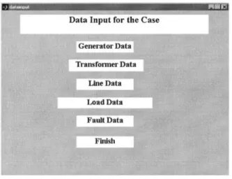
The package is started with typing ‘TransGUI’ at the MATLAB command prompt. The opening screen, with all the options, is shown in Fig. 1. The user can open a new/existing data case, the name of which is displayed in the centre of Fig. 1.

The user can save the case after making modifications. While saving or retriev-ing existretriev-ing data-cases, a dialog box is displayed which lists the files and directo-ries in the current directory from which the user can select. When the user clicks on Simulation followed by Options in Fig. 1, one can specify the various simulation options such as method of simulation, simulation interval, and other parameters, as shown in Fig. 2.

The user can have hypertext help to learn more about SIME and the package by clicking on the help menu of Fig. 1. This opens the help file in the familiar MATLAB help browser with hyperlinks. The user can enter the package by clicking on Simu-lation followed by Run TransGUI. The user will see a screen as shown in Fig. 3. If

the user selects the Input Data option, the user is asked to select which data is to be entered as shown in Fig. 4. If the user has already entered the data, he/she can modify it if required. The screens following Input Data and Modify Data are almost same, except that in case the user wants to modify the data, the existing values are displayed on the screen.

The data entered by the user are validated at every stage and the user receives appropriate messages in the message box. The overall logic behind this program works as discussed below.

Whenever the user inputs the data for Generators, Transformers, Lines, Loads, and the Fault, the data are stored in matrices called Gendata, Trdata, Linedata, Loadata and Faultdata, respectively. They are then saved onto the hard disk in the

Fig. 1 Schematic diagram of the study system.

filename as selected by the user from the save option in Fig. 1. In case the data are to be modified, they are first loaded into the memory clicking the Open existing data case option in Fig. 1. These data are made global to all functions. When the user selects Run Simulation option from Fig. 3, the program first forms Ybusmatrices Ybf,

Ydfand Yaffor prefault, during fault and after fault network conditions. These

matri-ces are made use of in the SIMULINK model file multimachine.mdl. Here, in this model, the Pelect S-function is used to calculate the electrical power output at every time step. Thus the code inside the Pelect S-function compares the simulation time with the fault time and clearing time and calculates the generator currents by using

Fig. 3 Simulation options.

the relationship I = Y·E where the appropriate value of Y is used. Real(E·I*) gives the electrical power. The electrical power thus obtained is subtracted from the gen-erator mechanical power to obtain accelerating power Pa. SIMULINK solves the

dif-ferential equations to obtain values of machine angles. The angles thus obtained at each time step along with inertia constants, electrical power outputs and mechani-cal power inputs are used as input by the S-function ‘SIME’ to obtain the OMIB parameters according to the algorithm mentioned above. Details of the SIMULINK model for calculating the time domain simulation and stability by the SIME tech-nique are given in the next section.

Stability simulation using SIMULINK

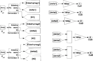
Figure 5 shows the part of the file ‘multimachine.mdl’ which is used to evaluate the stability by both SIME and T-D methods. In Fig. 5, each of the generators is mod-elled as a masked subsystem, which accepts electrical power injected into the gen-erator bus as the input and output values of voltage behind transient reactance (Edashq), M, and the value of delta at each time step.

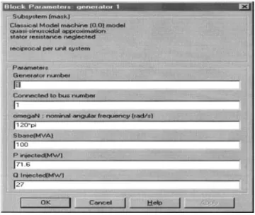
The inside of the masked subsystem is shown in Fig. 6. When the masked gen-erator system is double-clicked, the system prompts the user to enter the gengen-erator parameters as shown in Fig. 7.

The electrical power Peat every time instant is calculated by feeding the current

values of magnitudes and angles of voltages behind the transient reactance Edashqmag and delta respectively to a function Pelectwhich is an S-function written

in MATLAB. This function calculates the bus currents using relationship [I] = [Y]· [V] and then finds the real power by calculating the real part of [V] · [conj(I)] and returns a vector Pe. It is then de-multiplexed as Pe1, Pe2and Pe3and fed back to the

generator as the input. Writing this S-function makes the task much simpler as

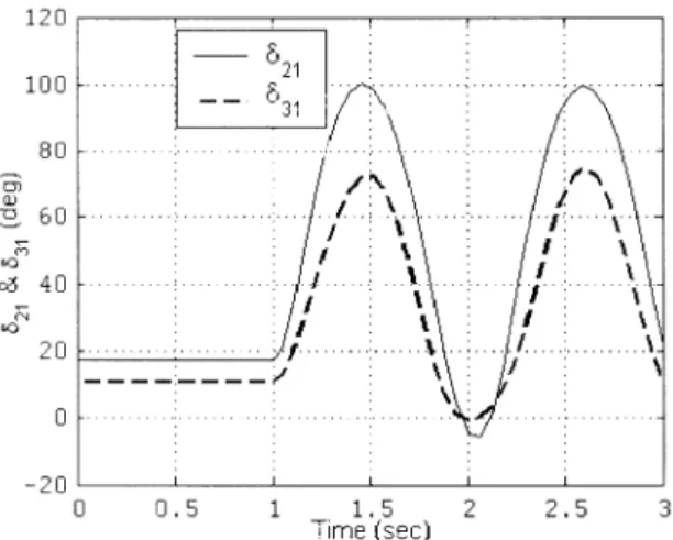
pared to generating in SIMULINK as has been done in Ref. 13. The output ports out1, out2, and out3 are used to store the values of absolute values of d1,d2and d3 in degrees. Out4 and out5 ports store the relative generator angles d21and d31 of generators 2 and 3 with respect to generator 1.

Figure 8 depicts a subsystem which accepts the absolute values of deltas and con-verts them with reference to the centre of angle reference frame. So output ports 6, 7, and 8 store the machine angles with respect to the COA reference frame.

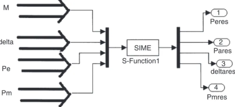
The algorithm for calculating the OMIBs at each step is written as a MATLAB S-function ‘SIME.s’. This function at each stage calculates the OMIBs. The

Fig. 6 Model for evaluating machine angle delta.

schematic for the SIMULINK block for doing this is shown in Fig. 9. M, delta, Pe, and Pm are vector signals having as many rows as the number of generators.

The values are fed at each time step in the SIME function S-block, which calcu-lates the OMIB parameters inside. Although parameters for all the OMIB parame-ters are calculated inside the SIME function only those for one OMIB are brought out here in this figure. Peresand Pmresare OMIB values for electrical and mechanical

power while Paresand deltares are OMIB values for accelerating power and machine

angle d. All the values are stored in vector yout and the simulation time is stored in vector tout during simulation. At the end of the simulation, the plots are obtained using the plot command.

Fig. 8 Initial parameters of a generator.

[delta1] [d1] [d2] Goto10 Goto11 Goto8 [d3] 8 7 6 2 1 180/PI 180/PI 180/PI Out3 Out2 Out1 In3 In2 In1 Subsystem1 [delta3] [delta2]

Gets o/p as COA

Simulation results

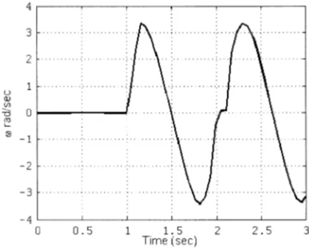
The results for the three-machine, nine-bus system (illustrated in Fig. 10), whose data are taken from Ref. 12, are shown for a fault near bus 7 at a line between bus 5 and 7. The fault occurs at 1 s and is cleared at 1.110 s (the actual clearing time is 0.110 s). The plots for the machine angle are shown in Figs 11, 12, and 13. In Fig. 11, absolute values of angles are plotted while in Fig. 12 the angles of generators 2 and 3 are plotted with reference to the angle of generator 1. In Fig. 13, the angles are plotted with the COA frame of reference. The plot for speed of the machine formed in the OMIB is shown in Fig. 14. The accelerating power (Pa) of the

equiv-alent OMIB is shown in Fig. 15.

It is clear from Fig. 11 that all the absolute angles of the generators are increas-ing and that they swincreas-ing almost together. This is also confirmed from Fig. 12 where the relative angle displacement with respect to generator 1 is shown.

Pmres deltares Pares 4 3 2 1 Peres S-Function1 SIME Pm Pe delta M

Fig. 10 SIMULINK block for calculating OMIB parameters.

However, plotting angle displacement relative to a generator and observing if the relative angles are in synchronism is not a confirmed test of stability. This is because it may so happen that the generator 1 is not in synchronism with respect to genera-tor 2 and 3. However since the generagenera-tors 2 and 3 are almost in synchronism with respect to each other, a plot of their relative angles with respect to generator 1 will also show synchronism. This can be avoided if one refers to a COA frame of refer-ence. This is shown in Fig. 13. So, one can see that all three generators are nearly in synchronism. The plot of speed of the equivalent OMIB is shown in Fig. 14. It can be seen that the speed after increasing is crossing the zero axis. If one observes the plot for accelerating power Paagainst time shown in Fig. 16, it can be seen that

the speed crosses zero earlier than the time at which the accelerating power starts

Fig. 12 Generator angles with respect to generator 1.

becoming greater than zero. This conforms to the theorem that the system is unsta-ble when Pa= 0 and dPa/dt > 0. In this case, although Pais becoming zero at around

t= 1.18s, it is decreasing and hence dPa/dt is negative.

The fact that the OMIB is stable is also clear from Fig. 16 where the electrical power Peafter reaching its peak, does not cross the line corresponding to

mechani-cal power input Pmech.

In fact, if one runs the simulation and sees the plot during runtime with the help of a scope, one can clearly observe the return trace from the point where the curve traces back after it has reached the maximum value of d.

Fig. 14 Speed of the equivalent OMIB.

Conclusions

This paper has proposed a user-friendly package to investigate transient stability. It relies on the SIME transient stability method together with the GUIDE tool of MATLAB and with SIMULINK. Through the use of scopes and plots the package has exhibited quite interesting capabilities: it has allowed clear observation as to how the system loses stability, and the severity and mode of instability; it can also assess the influence of various system parameters, suggest ways of stabilising the system, and provide a good insight into transient stability mechanisms. In short, the package shows to be a powerful didactic and research tool, able to provide impor-tant information about various aspects of transient stability phenomena. Incidentally, the package has also shown the superiority of SIME over the conventional T-D method.

Admittedly, the package developed in this paper can be considered as a startup tool, easily extensible in two main directions. One concerns incorporation of higher-order models of generators, loads, and the network itself. The other direction consists of augmenting the basic SIME software used in this paper with additional, already available software, such as FILTRA (contingency FILtering, Ranking, and Assessment),14_{or those developed for control (stabilisation).}15,16_{In fact, control} tech-niques are among the very unique assets of SIME and most useful tools. Work along these lines is underway.

Acknowledgement

The authors wish to acknowledge Prof. Thierry Van Cutsem and Dr. Damien Ernst, University of Liège, for useful discussions during the package development.

References

1 D. P. Kothari and I. J. Nagrath, Modern Power System Analysis, 3rd edn (Tata McGraw-Hill, New Delhi, 2003).

2 A. H. El-Abiad and K. Nagappan, ‘Transient stability region of multimachine power systems’, IEEE

Trans. PAS, PAS-85 (1966), 169–179.

3 M. Pavella, D. Ernst and D. Ruiz-Vega, Transient Stability of Power Systems – A Unified Approach

to Assessment and Control (Kluwer, Dordrecht, 2000).

4 T. Athey, R. Podmore and S. Virmani, ‘A practical method for direct analysis of transient stability’,

IEEE Trans. PAS, PAS-98 (1979), 573–584.

5 H. D. Chiang, F. F. Wu and P. P. Varaiya, ‘A BCU method for direct analysis of power system transient stability’, IEEE Trans. Power Syst., 9(3) (1994), 1194–1208.

6 Y. Zhang, L. Wehenkel, P. Rousseaux and M. Pavella, ‘SIME: A hybrid approach to fast transient stability assessment and contingency selection’, Intl J. Elec. Power Energy Syst., 19(3) (1997), 195–208.

7 Using SIMULINK ver. 5 (The Mathworks Inc., Natick, 2002).

8 MATLAB®_{– The Language of Technical Computing available online at http://www.mathworks.com} 9 Y. Y. Hsu, C. C. Yang and C. C. Su, ‘A personal computer based interactive software for power

system operation education’, IEEE Trans. Power Syst., 7(4) (1992), 1591–1597.

10 Z. Ao, R. J. Fleming and T. S. Sidhu, ‘A transient stability simulation package (TSSP) for teaching and research purposes’, IEEE Trans. Power Syst., 10(1) (1995), 11–17.

11 A. Z. Khan and F. Shahzad, ‘A PC based software package for the equal area criterion of power system transient stability’, IEEE Trans. Power Syst., 13(1) (1998), 21–26.

12 P. M. Anderson and A. A. Fouad, Power System Control and Stability (IEEE Press, Stevenage, 2003). 13 R. Patel, T. S. Bhatti and D. P. Kothari, ‘MATLAB/SIMULINK based transient stability analysis of

a multimachine power system’, Intl J. Elec. Enging Educ., 39(4) (2002), 320–336.

14 D. Ernst, D. Ruiz-Vega, M. Pavella, P. Hirsch and D. Sobajic, ‘A unified approach to transient sta-bility contingency filtering, ranking and assessment’, IEEE Trans. Power Syst., 16(3) (2001), 435–443.

15 D. Ruiz-Vega, M. Glavic and D. Ernst, ‘Transient stability emergency control combining open-loop and closed-loop techniques’, in Proc. IEEE PES General Meeting, Toronto, Canada, July 2003, pp. 2053–2059.

16 D. Ruiz-Vega and M. Pavella, ‘A comprehensive approach to transient stability control – Part I: Near optimal preventive control, Part II: Open loop emergency control’, IEEE Trans. Power Syst.,