Apprentissage statistique, variétés de formes et applications à la segmentation d'images

(1)

HAL Id: pastel-00004040

https://pastel.archives-ouvertes.fr/pastel-00004040

Submitted on 18 Jul 2008

HAL is a multi-disciplinary open access archive for the deposit and dissemination of sci-entific research documents, whether they are pub-lished or not. The documents may come from teaching and research institutions in France or abroad, or from public or private research centers.

L’archive ouverte pluridisciplinaire HAL, est destinée au dépôt et à la diffusion de documents scientifiques de niveau recherche, publiés ou non, émanant des établissements d’enseignement et de recherche français ou étrangers, des laboratoires publics ou privés.

applications à la segmentation d’images

Patrick Etyngier

To cite this version:

Patrick Etyngier. Apprentissage statistique, variétés de formes et applications à la segmentation d’images. Mathématiques [math]. Ecole des Ponts ParisTech, 2008. Français. �pastel-00004040�

(2)

, _{April 23, 2008 - Get an update.}_{http://certis.enpc.fr/∼etyngier/phd/dissertation}

Thesis

Submitted in partial fulfillment of the requirements for the degree of

Docteur de l’École Nationale des Ponts et Chaussées (ENPC). Spécialité Mathématiques, Informatique ( Doctor of Philosophy in Mathematics, Computer Science at ENPC )

Statistical learning, Shape Manifolds &

Applications to Image Segmentation

by

Patrick E

TYNGIER

Oral defense: January 21, 2008

PhD Committee: Nicholas AYACHE President

Daniel CREMERS Reviewer Rachid DERICHE

Françoise DIBOS Reviewer

Renaud KERIVEN PhD advisor

Bertrand THIRION

within the Odyssée Team

(3)

(4)

,

Thèse

Présentée pour l’obtention du grade de Docteur de l’École Nationale des Ponts et Chaussées

Spécialité: Mathématiques, Informatique

Apprentissage Statistique, Variétés de Formes &

Applications à la segmentation d’images

Par

Patrick E

TYNGIER

Soutenue le Lundi 21 Janvier 2008

Devant le jury composé de:

Nicolas AYACHE Président

Daniel CREMERS Rapporteur

Rachid DERICHE Examinateur

Françoise DIBOS Rapporteur

Renaud KERIVEN Directeur de thèse

Bertrand THIRION Examinateur

au sein de l’Équipe Odyssée

(5)

Abstract

Image segmentation with shape priors has received a lot of attention over the past few years. Most existing work focuses on a linearized shape space with small de-formation modes around a mean shape, which is only relevant when considering similar shapes. In this thesis, we introduce a new framework that can handle more general shape priors.

We model a category of shapes as a finite dimensional manifold, the shape prior manifold, which we analyze from the shape samples using dimensionality reduc-tion techniques such as diffusion maps. An embedding funcreduc-tion is then learned from the manifold. Unfortunately, this model does not provide an explicit projec-tion operator onto the underlying shape manifold, and therefore, our work tackles this problem.

Our solution is threefold.

First, we propose different solutions to the out-of-sample problem and define three attracting forces directed towards the manifold. These forces can be used as pro-jection operators onto the manifold:

• Projection towards the closest point • Projection with the same embedding • Projection at constant embedding

Next, we introduce a shape prior term for the active contours/regions framework through a non-linear energy term designed to attract shapes towards the manifold. Finally, we describe a variational framework for manifold denoising.

Results with real objects such as car silhouettes or anatomical structures show the potential of our method.

(6)

3

Resumé

La segmentation d’image avec a priori de forme a fait l’objet d’une attention par-ticulière ces dernières années. La plupart des travaux existants reposent sur des espaces de formes linéarisés avec de petits modes de déformations autour d’une forme moyenne. Cette approche n’est pertinente que lorsque les formes sont rel-ativement similaires. Dans cette thèse, nous introduisons un nouveau cadre dans lequel il est possible de manipuler des a priori de formes plus généraux.

Nous modélisons une catégorie de formes comme une variété de dimension finie, la variété des formes a priori, que nous analysons à l’aide d’échantillons de formes en utilisant des techniques de réduction de dimension telles que les diffusion maps. Un plongement dans un espace réduit est alors appris à partir des échantillons. Cependant, ce modèle ne fournit pas d’opérateur de projection explicite sur la var-iété sous-jacente et nous nous attaquons à ce problème.

Les contributions de ce travail se divisent en trois parties.

Tout d’abord, nous proposons différentes solutions au problème des "out-of-sample" et nous définissons trois forces attirantes dirigées vers la variété.

• Projection vers le point le plus proche;

• Projection ayant la même valeur de plongement; • Projection à valeur de plongement constant.

Ensuite, nous introduisons un terme d’a-priori de formes pour les coutours/régions actifs/ves. Un terme d’énergie non-linéaire est alors construit pour attirer les formes vers la variété.

Enfin, nous décrivons un cadre variationnel pour le debruitage de variété.

Des résultats sur des objets réels tels que des silhouettes de voitures ou des struc-tures anatomiques montrent les possibilités de notre méthode.

(7)

(8)

Remerciements /

Acknowledgment (French)

À mon directeur de thèse, Renaud Keriven

J’adresse toute ma reconnaissance à mon directeur de thèse, Renaud Keriven. Il a su en toutes circonstances, même celles qui me semblaient les plus désespérées, créer un climat de confiance et de sérénité qui m’a été particulièrement favorable. Je mesure la chance d’avoir été son étudiant et l’importance de l’expérience scien-tifique et humaine qu’il a partagée avec beaucoup de patience.

Aux chercheurs du CERTIS

Je remercie tous les chercheurs du CERTIS pour m’avoir éclairé de leur savoir au long des nombreux échanges et collaborations scientifiques. Je pense en particulier à Florent Ségonne, à Jean-Yves Audibert, à Jean-Philippe Pons, et à Hichem Sahbi. Je remercie également Nikos Paragios pour l’encadrement de qualité dont j’ai bénéficié lorsqu’il était à l’École des Ponts. Je n’oublie pas Yakup Genc avec qui j’ai collaboré à Siemens Corporate Research à Princeton, NJ aux Etats-Unis.

Aux membres du jury

Je suis conscient de l’honneur que m’ont fait les membres du jury par leur présence le jour de ma soutenance de thèse. En particulier, je remercie Daniel Cremers et Françoise Dibos, rapporteurs de ce manuscrit, Nicholas Ayache, président du jury, ainsi que Rachid Deriche et Bertrand Thirion, examinateurs.

(9)

Aux institutions

Je remercie les institutions qui ont organisé la logistique autour de cette thèse et qui ont assuré son bon déroulement. Il s’agit évidemment de l’École des Ponts -ParisTech mais aussi de la région Ile de France pour son soutien financier.

J’en profite pour remercier tous les contribuables qui ont indirectement participé au financement de ces 3 années de recherche.

A tous les membres du certis

Je remercie également tous les membres du CERTIS qui ont tous contribué à une bonne ambiance de travail, propice à la réussite.

(10)

7

A ma famille

Je profite de ces quelques lignes pour exprimer toute ma gratitude à mes parents, Jacques et Myriam, qui m’ont soutenu et encouragé durant toutes mes années d’études quels que soient les choix que j’ai pu faire. Je n’oublie pas mes frères et ma belle soeur, Philippe, Pascal et Jessica, ma grand-mère, Mimi, et mon oncle, Albert qui ont eu la patience d’être à mes côtés même durant mes moments insup-portables.

Aux amis

Je garde aussi un peu d’espace pour mes amis qui m’ont encouragé et écouté pen-dant des heures et des heures et qui m’ont fait l’honneur d’être présent le jour de la soutenance.

(11)

(12)

List of Figures

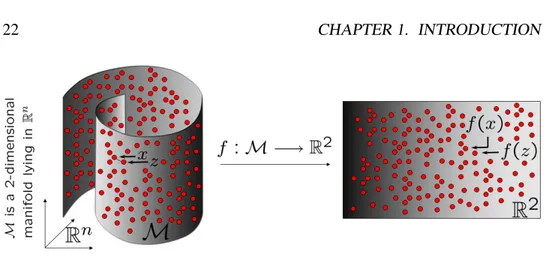
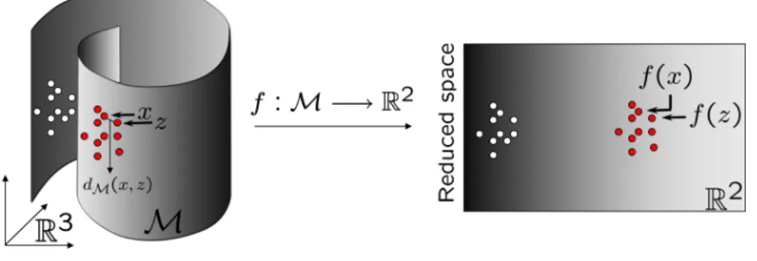
1.1 Non linear manifold learning techniques build an embedding func-tion f that represents the data in a lower dimensional space. Red points sample a non linear manifold. Linear models such as PCA or MDS cannot be applied to such non linear datasets as explained

in chapter 5. . . 22

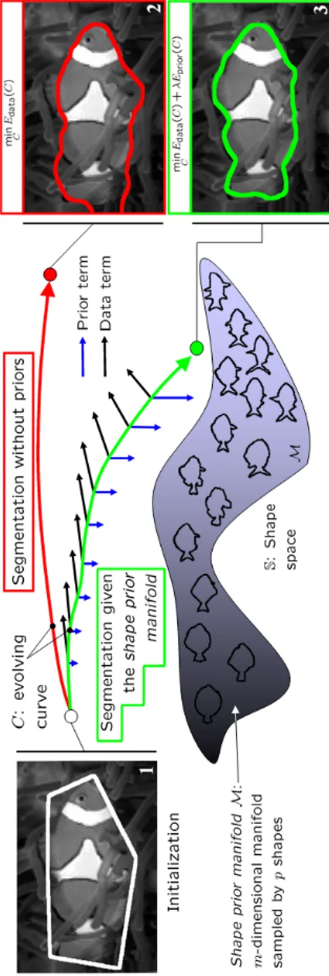
1.2 Overview and goal of this dissertation : a category of shapes — e.g. the fish shapes — is represented as a finite dimensional mani-fold. The shape prior term is a force directed toward the manifold

and combined with a data term force . . . 29

2.1 Les techniques d’apprentissage non linéaire de variété construisent

un plongement f qui représente les données dans un espace de plus petite dimension. Sur la figure ci-dessus, les points rouges échan-tillonnent une variété (non linéaire). Les modèles linéaires tels que ACP ou MDS ne peuvent pas être utilisés pour analyser de manière

fiable les ensembles non linéaires (Cf chapitre 5). . . 34

2.2 Vue d’ensemble de notre approche et but cette thèse: une caté-gorie de formes — e.g. les formes de poissons — est représentée comme une variété différentielle de dimension finie. L’a priori de

forme est une force dirigée vers la variété et est combiné avec une

force d’attache aux données. . . 40

3.1 Example of mesh for a half cylinder surface . . . 47

3.2 Representation of the unit circle as the isolevel of a scalar function 48

3.3 Mean Curvature Motion: Evolution of curves in the Level Set framework following equation (3.23): the shape becomes convex

and then disappears into a “circle point” in a finite time . . . 55

(17)

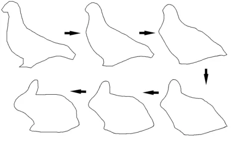
3.4 Interpolation in the shape space between two points (a bird and

a rabbit) using six weighted means.λ = 0, 0.2, 0.4, 0.6, 0.8 and 1 . 57

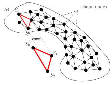
3.5 Local interpolation of the shape manifold M of dimension n:

weighted mean shapes are used to locally interpolate M within

a given n dimensional simplex (in red), that linearly and locally

approximates M . . . 58

4.1 Edge detectors - First Column: filter response Second Column: Thresholded filter response (thresholds automatically estimated) First row: Sobel operator, which estimates the gradient of the image. Single threshold: 11.11 Second row: Laplacian of Gaus-sian operator, detection of zero crossing. Single threshold: 0.43 Third row: Canny operator. Hysteresis thresholding, low thresh-old: 0.018, high threshthresh-old: 0.046 Fourth row: Deriche opera-tor. Hysteresis thresholding, low threshold: 0.012 , high threshold:

0.031 . . . 66

4.2 Perona-Malik diffusion: from left to right, original image, after

50 iterations and after 200 iterations . . . 69

4.3 Active snakes contours: from left to right, initialization of a snake, after convergence (original image), after convergence (norm of

in-tensity gradient image) . . . 71

4.4 Geometric active contours: Evolution in the level set framework following (Eq. 4.16). Bottom right image represents the function

g. Here g(x) = 1/1 + ||x||2 _{. . . .} ₇₃

5.1 Example of PCA in 2 dimensions . . . 84

5.2 PCA fails with “non linear data”: Black points are the data to be analyzed. The color code represents the values of the point projection onto the principal axes. Top: PCA Values on the first (left) and second (right) principal axis. Bottom: KPCA values on

the first (left) and second (right) principal axis . . . 85

5.3 The kernel trick: data mapping (from left to right) following ϕ(a, b) =_¡

a2_,√_{2ab, b}2¢ _{. . . .} ₈₆

5.4 Multi-Dimensional Scaling - On the left: Distance between two points using a distance in the data space. Applying MDS with such a distance would produce unexpected results. On the right:

(18)

LIST OF FIGURES 15

5.5 Dimensionality reduction - the embedding f preserves the local

information of the manifold M. . . 93

5.6 Diffusion maps - The diffusion distance D2

t(x, y) is approximated

by the Euclidean distance in the reduced space . . . 100

6.1 Top: the distribution of two classes corresponding to two indi-viduals. It is clear that the intra class variance is larger than the inter class one. Bottom: the distribution of the same classes in-side the manifold trained using graph Laplacian. It is clear that the converse is now true and the classification task is easier in the

embedding space. . . 110

6.2 Top: samples taken from the Swiss roll. On the left: A short cut makes the random walk Laplacian embedding very noise sensitive, clearly the variation of the color map does not follow the intrinsic dimension of the actual manifold. In the middle: when using the diffusion map, noisy paths affect the estimation of the conditional probabilities. On the right: when using the ro-bust diffusion map, the color map varies following the intrinsic

dimension. . . 115

6.3 Robustness of the embedding with respect to uniform noise through-out the curvilinear abscissa of the Swiss roll. From top to bottom,

the noise is 0%, 15% and 40%. . . 117

6.4 Means of interpolation error using the Nyström extension. In

green: errors on P0_{. In blue: errors on P \ P}0_. _{. . . 119}

6.5 On the top: These figures show the recall for Orl, Swedish and

Corel databases for different graph Laplacians. On the Bottom: Comparison of Graph Laplacian with respect to SVM, Parzen

and Graph-cuts. . . 120

7.1 The Snail algorithm: steps are indexed 1, 2, . . . , if . . . 131

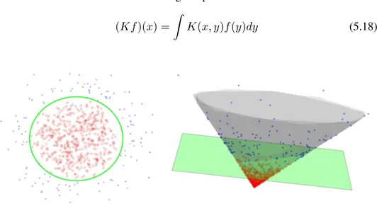
7.2 Projection onto the manifold: attracting forces # 2 & # 3 - a) Set of point samples lying on the surface given by the equation

f (x, y) = x2_{+ y}2_{. b) The reduced space and the Delaunay}

trian-gulation. c) Steepest descent evolution toward the weighted mean

Π2

M(x) (in blue) and at constant embedding (in red). The

Delau-nay triangulation is represented in the original space. d) Values of

(19)

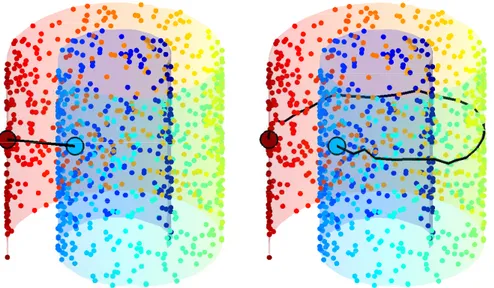
7.3 Being attracted toward the manifold (here, black dots) at con-stant embedding The color code represents the embedding value (also visualized along the z-axis on the right). The force #3 en-forces the point to be evolved toward the manifold by preserving

the embedding value. . . 137

7.4 Evolution toward the manifold at constant embedding value On the left: Sampled manifold (black dots) and visualization of the embedding value (color code). On the right: schematic detail. The blue line represents the set of point having the same embedding value as x. The force #2 modifies the embedding value during the evolution. The force #3 (red arrow in the tangent direction of the blue line) enforces the point x to evolve at constant embedding

value. . . 137

7.5 Three forces to attract points toward the manifold M . . . 138

8.1 Manifold Denoising - a) The set of point sample with the iso-level set of the one dimensional embedding. b) After 5 iterations of denoising. Smaller points correspond to original data, bigger to denoised data. The black lines are the paths of some randomly

points during the evolution c) Final result. . . 141

8.2 Projection onto the rectangle manifold using the snail algorithm

(attracting force #1 - direct projection): {S0, S1, S2} is the

neigh-borhood system . . . 144

8.3 Projection onto the fish manifold using the snail algorithm

(at-tracting force #1 - closest projection): {S0, S1, S2, S3} is the

neigh-borhood system . . . 145

8.4 Projection onto the cross manifold using the same embedding force (attracting force #2): On the top: Reduced space. The black points is the embedding of the altered shape. On the bottom:

Cor-rupted shape, its neighborhood system {S0, S1, S2}, and its

pro-jection. . . 150

8.5 The ventricle manifold: Comparison of the evolution toward the

Karcher mean shape Π2

M(· ) (in blue) and the evolution at constant

embedding(in red). The plane is represents the embedding

(20)

LIST OF FIGURES 17

8.6 The fish embedding: 2-dimensional representation of 150 fishes

[SQUID database]. . . 152

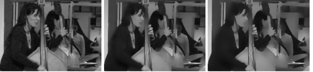
8.7 Fish segmentation - attracting force # 2 1: initial contour 2: active contour without shape prior 3: active contour with shape

prior 4: reprojection of the final result on the shape manifold . . . 153

8.8 Training set of the car manifold is made of 192 car shapes. It is comprised of 17 different cars (1 row ↔ 1 car ) : Audi A3, Audi TT, BMW Z4, Citroën C3, Chrysler Sebring, Honda Civic, Renault Clio, Delorean DMC-12, Ford Mustang Coupe, Lincoln MKZ, Mercedes S-Class, Lada Oka, Fiat Palio, Nissan 200sx , Nis-san Primera , Hyundai Santa Fe and Subaru Forester. For each car, 12 views are taken while turning around (1 column ↔ 1 view). Al-though we do complete a full turn, the manifold does not result in

a spherical topology. . . 154

8.9 Reduced space of the car data set and its Delaunay

triangula-tion. . . 155

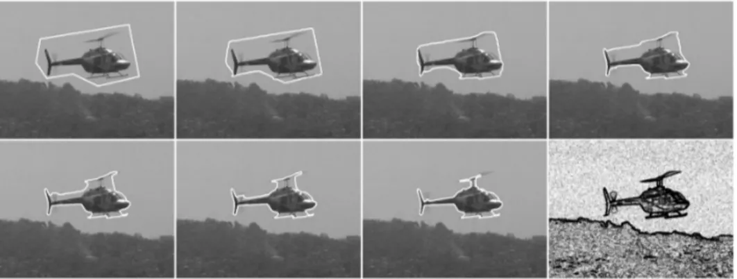
8.10 Segmentation with shape priors (car manifold), attracting force # 3 - Segmentation of a Peugeot 206 (left) and a Suzuki Swift (right). First row: Segmentation with data term only. Second row: segmentation with our shape prior. The embedding of the final shape is denoted by a blue cross and a green cross respectively for

the Peugeot 206 and the Suzuki Swift in Figure 8.9 . . . 156

8.11 Segmentation with shape priors (ventricle manifold), attract-ing force # 3, 1/2 - a) Eigenspectrum profile and degree of sep-arability: on this restricted data set with 39 shapes only, m = 2 appears to be the optimal dimension. b) The two-dimensional em-bedding partitioned by a Delaunay triangulation. c) A manually altered shape and its two closest neighbors in S and in the reduced

space: visually, the ones in the reduced space appear more similar. 157

8.12 Segmentation with shape priors (ventricle manifold), attract-ing force # 3, 2/2 - a) Coronal, horizontal, and sagital slices of the MRI volume with the final segmentations without (top) and with (bottom) the shape prior. b) Some snapshots of the shape evolution - the shape prior term was not used during the first steps. c) The

(21)

A.1 Parametrization of the Hough space . . . 170

A.2 Example of Hough Transform . . . 171

A.3 Discretization defects using standard Hough transform between

the two red lines. . . 172

A.4 Line signature in the Radon space for a given number of

consec-utive images. . . 173

A.5 Tracking lines in the Radon space and their projections in the corresponding image space. Results are presented in raster-scan

format.. . . 176

A.6 Overview of the proposed pose estimation approach where both

learning and estimation steps are delineated. . . 177

A.7 3D reconstruction of an indoor scene. . . 179

A.8 "Real" AdaBoost using stumps . . . 182

A.9 Error rates during 30 iterations of real AdaBoost - Top row: learning set. Bottom row: test set. Red: mean error - Blue: error rate of Class I, class of the line learnt - Green: error rate of Class

II, class of the other lines . . . 184

A.10 Example of learning results on synthetic data. Red lines:

match-ing of 3 lines usmatch-ing geometrical constraint . . . 186

A.11 Final calibration: the image to be calibrated is overlaid by the

(22)

Chapter 1

Introduction

Contents

1.1 Context . . . 19

1.1.1 On the image side. . . 19

1.1.2 On the statistical learning side . . . 20

1.2 Image segmentation and statistical learning . . . 22

1.3 Goal and organization of this dissertation . . . 23

1.1 Context

1.1.1 On the image side

Image analysis has enjoyed an increasing demand from the medical imaging field for a few years, since computer aided diagnostics rely mainly on image processing and computer vision techniques. Furthermore, images have now a predominant place in our daily life since camera devices appear everywhere. Cell phones all have one or two cameras embedded and the smallness constraint implies lower quality of optics and sensors, which is offset by an extensive use of image pro-cessing (image enhancements such as noise removal, automatic contrast balance etc.). Regular digital cameras have even real time face detectors to optimize the auto focus mode. Surveillance cameras in buildings, cities and highways have been considerably growing in number for the last two decades. In view of the huge

(23)

amount of video sequences produced, computer vision techniques can make the surveillance operations [semi-]automatic instead of costly numerous surveillance operators.

Image processing and computer vision are the sciences that analyze and ex-tract useful information from digital images and videos. An image is basically a n-dimensional array (in general, n = 2 or possibly n = 3. n is the dimension of the image domain) of which the values are quantified within a given range. Such values may be of dimension 1 (black and white images), 3 (color images) or even higher. Image processing is related to low-level vision tasks such as edge and con-tour extraction, noise removal, deblurring etc; while computer vision is related to higher level tasks such as object tracking in video, event detection in video, 3D reconstruction from 2D images, shape recognition etc. The latter relies of course on the former.

Researchers and manufacturers have been developing these techniques since the emergence of computers in the seventies. At that time, the techniques proposed were mainly low level based. Nevertheless, the core idea of image analysis has remained the same since its beginnings. Algorithms mostly attempt to partition images into components or areas of interest in order to do some kind of high level “intelligent process”. For example, edge detection algorithms partition an image into edge pixels and non edge pixels, shape recognition extracts an area of the image domain within a given range of shapes, object tracking does the same in video sequences etc. All these processes can be called image segmentation in the broad sense of the word. In this thesis, we will be focusing on application on active contour segmentation — i.e. extraction of objects in images by detecting their closed contour — and unless specified, we will implicitly refer to that kind of segmentation.

1.1.2 On the statistical learning side

As the number of computers over the planet and their storage capacity have con-siderably increased, they produce more and more data, which enable the devel-opment of huge database. Management, organization and understanding of such amounts of data cause many challenging problems to tackle. Statistical approaches are commonly used when dealing with such databases, particularly in the fields of

(24)

1.1. CONTEXT 21 classification and dimensionality reduction.

Classification is the science that classifies data into two or more clusters. First, it extracts features from data with some invariant characteristics. A classification function is then learned from a set of training samples and its capacity to generalize to new samples is assessed using a test set ( of course with distinct samples from the training set). An efficient learning algorithm for classification should minimize two different errors called learning error and generalization error. The former is the error made on the training set while the latter is the error made on the test set. The more complex the function is, the less the learning error is, but the more the generalization error might be. A trade-off between the two errors should then be determined.

Dimensionality reduction techniques deal with high dimensional data and aim to represent them in a lower dimensional space to have a better understanding of their intrinsic characteristics, ideally to recover their intrinsic parametrization. They typically build a mapping from the original space into the lower dimensional space. The premises date back to the beginning of the twentieth century when Kenneth Pearson introduced the Principal Component Analysis technique (PCA) [151] in 1901. PCA assumes that data lie on a linear subspace under a Gaus-sian distribution. Multi-Dimensional Scaling (MDS) is another linear technique related to PCA, based on pair-wise distance in the dataset [216,201,51]. For the last decade, dimensionality reduction has received interest because many problems cannot be modeled using linear models. A non linear version of PCA was proposed in [180] by using kernel methods. In addition, a series of recent techniques relies explicitly on the assumption that data lie on a (non linear) smooth manifold. These approaches, which are particularly successful because of their well-posedness, are also known as manifold learning techniques. Among the most popular techniques are Locally Linear Embedding (LLE) [166], Laplacian Eigenmaps [99] and Dif-fusion maps [117]. These methods are able to output a low dimensional global representation of high dimensional data lying on a non linear manifold by preserv-ing the local neighborhood information, and can be possibly extended to new data.

In both cases, the learning function should be estimated from a training set of limited size and should have good generalization capacities.

(25)

Figure 1.1: Non linear manifold learning techniques build an embedding function f that represents the data in a lower dimensional space. Red points sample a non linear manifold. Linear models such as PCA or MDS cannot be applied to such non linear datasets as explained in chapter5.

1.2 Image segmentation and statistical learning

The goal of image segmentation is basically to partition the image domain into N disjoint regions that usually correspond to part or complete objects in the scene. In earlier approaches, image segmentation methods delineated objects by using only their edges, which are identified by higher gradient values in the target im-age. Regions of the image domain can also, for instance, be guessed according to given pixel grouping constraints (uniformity, statistical properties etc., within the regions).

In this work, we are limited to two regions separated by a boundary contour. With-out loss of generality, many approaches define a curve denoted S which minimizes a given energy functional. For example, graph cuts find the curve that has the global minimum of the energy. In this thesis, we focus on gradient descent ap-proaches in order to minimize the target energy functional: the curve S evolves on the image domain according to the minimization of a variational energy E. An en-ergy Edatais usually designed to attract the curve S toward the edges of the object

to segment. Edatacan also, for example, be designed regarding the statistical

prop-erties inside and outside the curve S. See section (4.3.3) for region-based active contour segmentation.

(26)

1.3. GOAL AND ORGANIZATION OF THIS DISSERTATION 23 Edges may be badly defined due to blur, noise, or occlusion and a smoothness constraint E_smooth along the curve S must be added to equation (2.1) to overcome such difficulties. Nevertheless, it is not sufficient and an a-priori knowledge on the possible shapes must also be introduced. Statistical learning is extensively used in computer vision in order to introduce an a-priori knowledge, particularly in image segmentation processes. In this work, we focus on shape priors learned from a given training set. Segmentation with shape priors is expressed using a model similar to equation (2.1), but new energies Ea-prioriand Esmoothare added. Ea-priori,

built from the training set, constrains the curve within a given range of shapes, while Esmoothconstrains the curve to be smooth.

E₂(S) = E_data(S) + αE_smooth(S) + βE_a-priori(S) (1.2) where α and β are parameters set to quantify the influence of the a-priori knowl-edge and the smoothness of the curve in the final result. To our best knowlknowl-edge, the work by Daniel Cremers, Cristoph Schnörr, Joachim Weickert and Christian Schellewald on Diffusion Snakes [58,57] was the first to combine a generic seg-mentation method with an added energy.

1.3 Goal and organization of this dissertation

There are many attempts in literature to embed a-priori knowledge in segmenta-tion tasks notably by using dimensionality reducsegmenta-tion techniques, as in the work of Michael Leventon, Eric Grimson and Olivier Faugeras in [122] but also in [165,42,203,40] to cite a few. These approaches assume that data lie on a linear subspace under a Gaussian distribution.

In this work, we want to depart from such assumptions in order to handle more general non linear shape priors. We model a category of shape — e.g. the category of fish shapes — as a smooth non linear finite dimensional manifold that we call the shape prior manifold. In this context, our view is that the shape priors is a force directed toward the shape prior manifolds. An important related work was proposed by Daniel Cremers, Timo Kohlberger and Christoph Schnörr in [53]. The authors introduce non linear shape priors by using a probabilistic version of Kernel PCA (KPCA). Note that we aim to handle more general cases.

(27)

Although we are driven by applications for image segmentation with shape pri-ors in this work, we will endeavor to present our contribution in a generic form. The purpose of this dissertation is to extend cutting edge manifold learning techniques such as diffusion maps to design a force that attracts data toward the manifold. The force should be designed to be usable in the context of image segmentation. An overview of the concept is presented in figure (2.2).

This thesis is organized as follow.

Chapter3: Shapes

This chapter provides the reader with all the necessary background about shapes. In particular, we define the concept of shape and detail some of their possible representations. We also introduce the notion of distance between shapes. Finally, we explain how to interpolate between shapes by using for instance Karcher means [107] and how to model a shape manifold from a finite shape set.

Chapter4: Image segmentation

In this chapter, we briefly review the techniques of image segmentation in the broad sense of the word. Since we are driven by applications in image segmentation, we give the context to show how our approach crosses over a new step in the state of the art.

Chapter5: Dimensionality reduction and non linear manifold learning

In our work, we aim to learn shape priors from a category of shapes lying on a non-linear smooth manifold. Chapter5focuses on the statistical learning side and on dimensionality reduction techniques, which define an embedding into the reduced space. This chapter is organized to emphasize the needs and the importance of non linear models. We present and illustrate the most popular methods from basic linear models such as PCA [151] or MDS [201,202,51] to cutting edge non linear manifold learning techniques such as Laplacian eigenmaps [15] and diffusion maps [117].

(28)

1.3. GOAL AND ORGANIZATION OF THIS DISSERTATION 25

Chapter6- Application I: Interactive image retrieval

Since our work relies mainly on manifold learning techniques, we focus on an application of graph Laplacian/diffusion maps to interactive image retrieval based on relevance feedback techniques. In these approaches, the system attempts to build a metric and/or a decision rule that reflects the user’s intention based on not only the data he labeled but also the others (usually the user does a binary labeling). Indeed, data are supposed to lie on a smooth manifold and diffusion maps are used to learn this manifold and diffuse the labels (this process is known as transductive learning). An interaction between the system and the users is then created in order to refine the response by proposing new unlabeled data to the user. Finally, the system outputs a class of images supposed to reply to a query defined by the user’s mind.

Publications related to this chapter

Hichem Sahbi, Patrick Etyngier, and Jean-Yves Audibert and Renaud Keriven. Graph Laplacian for Interactive Image Retrieval. ICASSP’ 08: In proceedings of the International Conference on Acoustics, Speech, and Signal Processing, Las Ve-gas, April 2008.

Hichem Sahbi, Patrick Etyngier, and Jean-Yves Audibert and Renaud Keriven. Manifold Learning using Robust Graph Laplacian for Interactive Image Retrieval. CVPR’ 08: In proceedings of the IEEE International Conference on Computer Vi-sion and Pattern Recognition, Anchorage, Alaska, June 2008.

Chapter7: Extensions and attracting forces

This chapter contains the main contributions of this dissertation. Our approach relies on a manifold learning techniques called diffusion maps, that builds an em-bedding function into a low dimensional representation of data. This mapping is defined only on the training samples. Chapter7starts by pointing out extensions of the embedding to any new point — i.e. outside the training set — that comes into the process. Such extensions avoid recalculating embedding values from scratch.

(29)

mani-fold. A natural idea is to design a projection operator onto the manifold in order to obtain an attracting force.

We propose three different attracting forces in this chapter. The first one is based on a projection minimizing the distance to the manifold. Next, the second force relies on a projection having the same embedding value. We finally define a third attracting force toward the manifold, which preserves the embedding con-stant. This latter approach, which relies on diffusion maps [117] and the Nyström extension [145], is well posed and natural.

Again, since the tools developed in this work can be applied to any kind of data lying in a space equipped with a differentiable distance, we endeavor to present this chapter in a generic form.

Patrick Etyngier, Renaud Keriven, and Jean-Philippe Pons. Towards segmentation based on a shape prior manifold SSVM’ 07: In proceedings of the 1st International Conference on Scale Space and Variational Methods in Computer Vision Ishia, Italy, May 2007.

Patrick Etyngier, Renaud Keriven and Florent Ségonne. Projection Onto a Shape Manifold for Image Segmentation with Prior. ICIP’ 07: In proceedings of the 14th IEEE International Conference on Image Processing, San Antonio, Texas, USA, September 2007.

Patrick Etyngier, Renaud Keriven and Florent Ségonne. Shape priors using Man-ifold Learning Techniques. ICCV’ 07: In proceedings of the 11th IEEE Interna-tional Conference on Computer Vision, Rio de Janeiro, Brazil, October, 2007. Patrick Etyngier, Renaud Keriven and Florent Ségonne. Active-Contour-Based Image Segmentation using Machine Learning Techniques. MICCAI’ 07: In pro-ceedings of the 10th International Conference on Medical Image Computing and Computer Assisted Intervention, Brisbane, Australia, October, 2007

(30)

Chapter8- Application II: Manifold denoising and image segmentation with general non linear shape priors

The tools developed in chapters5and7of this dissertation are successfully applied to manifold denoising and image segmentation with non linear shape priors. In particular, chapter 8illustrates results obtained on various 2D and 3D examples corresponding to different shape manifolds: fishes, cars and anatomical structures.

Patrick Etyngier, Renaud Keriven, and Jean-Philippe Pons. Towards segmentation based on a shape prior manifold SSVM’ 07: In proceedings of the 1st International Conference on Scale Space and Variational Methods in Computer Vision Ishia, Italy, May 2007.

Patrick Etyngier, Renaud Keriven and Florent Ségonne. Projection Onto a Shape Manifold for Image Segmentation with Prior. ICIP’ 07: In proceedings of the 14th IEEE International Conference on Image Processing, San Antonio, Texas, USA, September 2007

Patrick Etyngier, Renaud Keriven and Florent Ségonne. Shape priors using Man-ifold Learning Techniques. ICCV’ 07: In proceedings of the 11th IEEE Interna-tional Conference on Computer Vision, Rio de Janeiro, Brazil, October, 2007 Patrick Etyngier, Renaud Keriven and Florent Ségonne. Active-Contour-Based Image Segmentation using Machine Learning Techniques. MICCAI’ 07: In pro-ceedings of the 10th International Conference on Medical Image Computing and Computer Assisted Intervention, Brisbane, Australia, October, 2007.

AppendixA: Radon/Hough space for pose estimation

In this appendix, we present a learning based approach to one shot camera cali-bration. First, features based on the Radon/Hough transform are learned while 3D reconstruction of a given indoor scene is achieved. An inference step then deter-mines the position of a one-shot image from its features and the 3D reconstruction.

(31)

Publication related to this chapter

Patrick Etyngier, Nikos Paragios, Renaud Keriven, Yakup Genc and Jean-Yves Au-dibert. Radon space and Adaboost for Pose Estimation. ICPR’ 06: In proceedings of the 18th International Conference on Pattern Recognition Hong-Kong, August 2006.

(32)

Figure 1.2: Overview and goal of this dissertation: a category of shapes — e.g. the fish shapes — is represented as a finite dimensional manifold. The shape prior term is a force directed toward the manifold and combined with a data term force

(33)

(34)

Chapitre 2

Introduction (Version française)

Contents

2.1 Contexte . . . 31

2.1.1 L’image comme point de départ . . . 31

2.1.2 L’apprentissage statistique comme point de départ . . 33

2.2 Segmentation d’image et apprentissage statistique . . . 34

2.3 But et organisation de ce manuscrit . . . 36

2.1 Contexte

2.1.1 L’image comme point de départ

Depuis quelques années, l’analyse d’image est de plus en plus sollicitée par les applications d’imagerie médicale, puisque les diagnostics médicaux assistés par ordinateur reposent principalement sur les techniques de traitement d’image et de vision par ordinateur.

Par ailleurs, les images numériques ont pris une place prédominante dans notre vie quotidienne où les caméras vidéo et appareils photos deviennent omniprésents. Les téléphones portables intègrent tous une voire deux capteurs. La contrainte de taille entraîne une qualité amoindrie des optiques et des capteurs, compensée par l’utilisation intensive de traitement d’image (amélioration de l’image tel que la réduction du bruit, réglage automatique du contraste etc. ). Désormais, même les

(35)

appareils photos non professionnels ont des détecteurs de visage en temps réel pour optimiser l’autofocus.

Aussi, le nombre de caméras de surveillance a explosé depuis les vingt der-nières années dans les bâtiments publics et privés, dans les villes, sur les auto-routes etc. . . Face à la quantité de séquences vidéo produite quotidiennement, les techniques de vision par ordinateurs peuvent rendre les opérations de surveillance beaucoup moins coûteuses, en réduisant par exemple le nombre d’opérateurs né-cessaires grâce à l’automatisation des processus.

Le traitement d’image et la vision par ordinateur sont les sciences qui ana-lysent et extraient des informations utiles des images et vidéo numériques. Une image est un tableau de dimension n (en général, n = 2 ou parfois n = 3. n est la dimension du domaine de l’image), dont les valeurs sont quantifiées dans un inter-valle borné. Ces valeurs peuvent être de dimension 1 (images en “noir et blanc”), 3 (image en “couleur”) ou parfois de dimension supérieure.

Le traitement d’image est un ensemble de techniques qui réalisent des tâches de vision bas niveau tels que l’extraction de bords et de contours, la réduction de bruit, le défloutage etc, tandis que la vision par ordinateur est un ensemble de techniques qui réalisent des tâches de vision de niveau plus élevé, telles que le suivi d’objet et la détection d’événements dans les vidéo, la reconstruction 3D à partir d’images 2D, la reconnaissance de formes etc. . . . La vision par ordinateur repose naturellement sur les techniques de traitement d’images.

Les chercheurs et industriels ont développé ces techniques depuis l’émergence des ordinateurs dans les années 70. A cette époque, les techniques étaient princi-palement de bas niveau. Cependant, l’idée de base de l’analyse d’image est restée inchangée depuis ses débuts. Les algorithmes tentent, pour la plupart, de morceler le domaine de l’image en composantes ou régions d’intérêt, afin de réaliser des “processus intelligents” de haut niveau. Par exemple, les algorithmes de détection des bords séparent les pixels appartenant aux bords et les autres, les algorithmes de reconnaissance de forme extraient une région de l’image contrainte dans un en-semble donné de formes, le suivi d’objet a les mêmes objectifs dans les séquences vidéo etc. Tous ces processus sont appelés segmentation d’image au sens large du terme. Dans cette thèse, nous nous concentrerons sur la segmentation par contours actifs — i.e. l’extraction d’objets dans les images en utilisant leur contour — et sauf mention contraire, nous ferons implicitement référence à ce type de

(36)

segmen-2.1. CONTEXTE 33 tation.

2.1.2 L’apprentissage statistique comme point de départ

Alors que le nombre d’ordinateurs sur la planète et leur capacité de stockage ont considérablement augmenté, de plus en plus de données nourrissent des bases de données énormes. La gestion, l’organisation et la compréhension de telles quan-tités de données suscitent des nouveaux défis à relever, particulièrement dans les domaines de la classification et de la réduction de dimension.

La classification est la science qui classe les données en deux (ou plus) en-sembles. D’abord, des caractéristiques invariantes sont extraites des données. Une fonction de classification est alors apprise à partir d’un ensemble d’apprentissage et sa capacité à généraliser à de nouveaux échantillons est évaluée au moyen d’un ensemble test (dont les échantillons sont évidemment distincts de ceux contenus dans l’ensemble d’apprentissage). Un algorithme d’apprentissage efficace pour la classification doit minimiser deux erreurs appelées erreur d’apprentissage et erreur de généralisation. L’erreur d’apprentissage est l’erreur faite sur l’ensemble d’ap-prentissage tandis que l’erreur de généralisation est l’erreur faite sur l’ensemble de test. Plus la fonction de classification est complexe, plus l’erreur d’apprentissage est petite, mais plus l’erreur de généralisation est importante. Un compromis entre les deux erreurs doit donc être trouvé.

Les techniques de réduction de dimension ont pour objectif de représenter des données de grande dimension dans un espace de plus petite dimension, afin de d’en extraire des caractéristiques intrinsèques, idéalement pour retrouver leur pa-ramétrisation intrinsèque. Pour cela, il faut construire une application de l’espace original des données vers un espace de plus petite dimension. Les prémisses re-montent au début du vingtième siècle avec l’analyse en composante principales (ACP) introduite par Kenneth Pearson en 1901 [151]. L’utilisation de l’ACP sup-pose que les données analysées sont sur un sous-espace linéaire selon une distri-bution gaussienne. Il existe également une autre approche linéaire, sous le nom de Multi-Dimensional Scaling (MDS), proche de l’analyse en composante principale mais qui construit une application dans un espace de plus petite dimension à par-tir des distances entre les points uniquement [216, 201,51]. Depuis une dizaine d’années, la réduction de dimension a connu un regain d’intêret car beaucoup de

(37)

problèmes ne peuvent être résolus à l’aide des méthodes linéaires. Une version non linéaire de l’analyse en composante principale a été proposée en utilisant les mé-thodes à noyaux : l’analyse en composante principale à noyau [180]. Par ailleurs, une série de techniques récentes reposent explicitement sur l’hypothèse que les données échantillonnent une variété différentiable (non linéaire). Parmi ces mé-thodes, on trouve : Linear Embedding (LLE) [166], Laplacian Eigenmaps [99] et Diffusion maps [117]. Ces méthodes sont capables de représenter globalement des données de grande dimension échantillonnant une variété différentielle, en pré-servant uniquement l’information locale de voisinage. L’extension aux nouveaux points est possible.

Dans les deux cas, la fonction d’apprentissage doit être estimée à partir d’un ensemble de points (ensemble d’apprentissage) de taille limitée et doit avoir de bonnes capacités de généralisation.

FIG. 2.1 – Les techniques d’apprentissage non linéaire de variété construisent

un plongement f qui représente les données dans un espace de plus petite dimen-sion. Sur la figure ci-dessus, les points rouges échantillonnent une variété (non linéaire). Les modèles linéaires tels que ACP ou MDS ne peuvent pas être utilisés pour analyser de manière fiable les ensembles non linéaires (Cf chapitre5).

2.2 Segmentation d’image et apprentissage statistique

Le but de la segmentation est de diviser le domaine d’une image en N régions disjointes qui correspondent, en général, à des objets partiels ou complets.

(38)

2.2. SEGMENTATION D’IMAGE ET APPRENTISSAGE STATISTIQUE 35 Historiquement, la segmentation d’image délimitait les objets en utilisant uni-quement leurs bords, où les valeurs du gradient de l’image sont maximales. Les régions du domaines de l’image peuvent aussi, par exemple, être détectées selon des contraintes de regroupements de pixels (uniformité, propriétés statistiques etc . . . à l’intérieur de la région).

Dans ce travail, nous nous limitons à deux régions séparées par un contour. Beau-coup d’approches définissent une courbe, notée S, qui minimise une énergie. Par exemple, les graph cuts trouvent la courbe qui a le minimum global de l’énergie. Dans cette thèse, nous nous utiliserons principalement des approches variation-nelles par descente de gradient afin de minimiser une fonctionnelle d’énergie : on fait évoluer la courbe S sur le domaine de l’image de manière à minimiser une énergie variationelle E. En général, on écrit une énergie Edataqui attire la courbe

S vers les bords de l’objet à segmenter. Les propriétés statistiques à l’intérieur ou à l’extérieur de la courbe peuvent également être utilisées pour décrire l’énergie Edata. Voir la section (4.3.3) pour la segmentation par contour actifs basée sur les

régions.

E1(S) = Edata(S) (2.1)

Les bords dans images sont parfois mal définis car flous, bruités ou recouverts par d’autres objets. Une contrainte de lissage Esmooth s’impose alors le long de

la courbe. Cependant, une telle contrainte n’est en général pas suffisante et un a priori sur les formes possible doit être introduit. L’apprentissage statistique est utilisé de manière intensive en vision par ordinateur pour introduire des a priori, particulièrement dans les processus de segmentation d’image.

Dans ce travail, nous nous concentrons sur l’apprentissage d’a priori de formes à partir d’un ensemble de formes. La segmentation avec a priori de formes s’écrit mathématiquement à l’aide d’un modèle similaire, mais avec l’ajout d’une nou-velle énergie Ea priori. Ea priori, construite à partir d’un ensemble d’apprentissage,

contraint la courbe dans un ensemble de formes possibles.

E₂(C) = E_data(C) + λE_{a priori}(C) (2.2) où λ est un paramètre qui quantifie l’influence ou la contribution de l’a priori dans le résultat final de segmentation. A notre connaissance, les travaux de Da-niel Cremers, Cristoph Schnörr, Joachim Weickert et Christian Schellewald sur les Diffusion Snakes [58,57] sont les premiers à combiner une segmentation avec un

(39)

terme d’énergie supplémentaire.

2.3 But et organisation de ce manuscrit

De nombreux articles en segmentation d’image utilisent des a priori de forme à l’aide de techniques de réduction de dimensions. On trouve par exemple les tra-vaux de Michael Leventon, Eric Grimson et Olivier Faugeras in [122], mais aussi [165,42,203,40]. Cependant, ces approches supposent que les données sont sur un sous-espace linéaire selon une distribution gaussienne.

Dans ce travail, nous voulons sortir de l’hypothèse gaussienne afin d’obtenir des a priori de formes plus généraux, non linéaires. En particulier, nous modélisons une catégorie de formes — e.g. la catégorie des formes de poissons — comme une variété différentielle de dimension finie, non linéaire, que nous appelons la variété des formes a priori. Dans ce contexte, nous considérons que l’a priori de formes est une force dirigée vers la variété des formes a priori.

Bien que nous souhaitions manipuler des cas plus généraux, nous attirons l’at-tention du lecteur sur des travaux connexes proposés par Daniel Cremers, Timo Kohlberger et Christoph Schnörr [53]. Les auteurs introduisent des a priori de forme non linéaires en utilisant une version probabilistique de l’ACP à noyaux (KPCA).

L’objectif de cette thèse est d’étendre les techniques d’apprentissage de variété tels que les diffusion maps, et de créer une force qui attire des points vers la variété. Cette force doit être conçue pour être utilisable dans le contexte de la segmentation d’image. La contribution de cette thèse sera présentée dans une forme générique alors que les applications gardent une place importante. Notre approche est illus-trée sous la forme d’un schéma, en figure2.2.

Dans la suite, nous décrivons l’organisation de cette thèse.

Chapitre3

Ce chapitre donne au lecteur les connaissances de base pour travailler avec des formes. En particulier, nous définissons le concept de forme et nous détaillons

(40)

2.3. BUT ET ORGANISATION DE CE MANUSCRIT 37 quelques représentations possibles. Nous introduisons également la notion de dis-tance entre formes. Enfin, nous expliquons comment interpoler entre les formes en utilisant des moyennes pondérées de forme.

Chapitre4

Dans ce chapitre, nous passons en revue les techniques de segmentation d’image, au sens large du terme. Puisque les contributions de cette thèse ont été guidées par des applications en segmentation d’image, nous présentons le contexte et nous montrons comment notre approche franchit une nouvelle étape dans l’état de l’art.

Chapitre5

Dans ce travail, l’objectif est d’apprendre des a priori de forme non linéaires à partir d’une catégorie de formes situées sur une variété différentielle. Le cha-pitre5se concentre sur l’apprentissage statistique, en particulier les méthodes de réduction de dimensions. L’organisation de chapitre est conçue pour souligner les besoins et l’importance de modèles non linéaires. Nous présentons et illustrons les méthodes les plus populaires depuis l’analyse en composante principales [151] ou le Multi-dimensional Scaling [201,202,51] jusqu’aux dernières techniques d’ap-prentissage non-linéaire de variétés, telle que les Laplacian maps [15] et diffusion maps [117].

Chapter6- Application I : Extraction intéractif d’image

Cette thèse repose principalement sur les techniques d’apprentissage de va-riété. Nous proposons donc une application des Laplaciens de graphe / diffusion maps, l’extraction intéractive d’images dans le cadre des techniques de relevance feedback. Dans ces approches, le système construit une métrique / règle de déci-sion qui reflète les intentions de l’utilisateur, à partir de données étiquetées ou non (en général, l’utilisateur étiquette quelques données de manière binaire). En effet, nous supposons que les données échantillonnent une variété différentielle et les diffusion maps sont utilisés pour apprendre cette variété et diffuser les étiquettes (ce processus porte le nom d’apprentissage transductif). Une intéraction entre le système et l’utilisateur est alors créée afin de raffiner la réponse en proposant de nouveaux points non étiquetées à l’utilisateur. Finalement, le système renvoie une classe d’image censée répondre à la requête formulée dans l’esprit de l’utilisateur.

(41)

Publications liées à ce chapitre

Hichem Sahbi, Patrick Etyngier, and Jean-Yves Audibert and Renaud Keriven. Graph Laplacian for Interactive Image Retrieval. ICASSP’ 08 : In proceedings of the International Conference on Acoustics, Speech, and Signal Processing, Las Ve-gas, April 2008.

Hichem Sahbi, Patrick Etyngier, and Jean-Yves Audibert and Renaud Keriven. Ma-nifold Learning using Robust Graph Laplacian for Interactive Image Retrieval. CV-PR’ 08 : In proceedings of the IEEE International Conference on Computer Vision and Pattern Recognition, Anchorage, Alaska, June 2008.

Chapitre7:

Ce chapitre contient nos principales contributions. Notre approche repose sur une technique d’apprentissage de variété, les diffusion maps, qui construisent un plongement (i.e. une application) vers une représentation des données dans un es-pace de plus petite dimension. Le plongement, est défini seulement sur les échan-tillons de l’ensemble d’apprentissage. Le chapitre 5 présente d’abord les possibili-tés d’extension du plongement aux nouveaux points —i.e. en dehors de l’ensemble d’apprentissage. Ces extensions évitent de recalculer toute l’application plonge-ment.

Notre but est de construire une force appliquée aux données, dirigée vers la variété apprise. L’idée naturelle est de construire un opérateur de projection pour obtenir une cible.

Nous proposons trois forces attractives dans ce chapitre. La première repose sur une projection minimisant la distance à la variété. Ensuite, la deuxième force repose sur une projection ayant la même valeur de plongement. Nous définissons enfin une troisième force attractive dirigée vers la variété qui préserve le plonge-ment constant. Cette dernière approche, qui repose sur les diffusion maps [117] et l’extention de Nyström [145], est bien posée et naturelle.

Puisque les outils développés dans ce travail peuvent être appliqués à toute sorte de données équipées d’une distance différentiable, nous nous efforcerons de présenter ce chapitre dans une forme générique.

(42)

2.3. BUT ET ORGANISATION DE CE MANUSCRIT 39 Publications liées à ce chapitre

Patrick Etyngier, Renaud Keriven, and Jean-Philippe Pons. Towards segmentation based on a shape prior manifold SSVM’ 07 : In proceedings of the 1st Internatio-nal Conference on Scale Space and VariatioInternatio-nal Methods in Computer Vision Ishia, Italy, May 2007.

Patrick Etyngier, Renaud Keriven and Florent Ségonne. Projection Onto a Shape Manifold for Image Segmentation with Prior. ICIP’ 07 : In proceedings of the 14th IEEE International Conference on Image Processing, San Antonio, Texas, USA, September 2007.

Patrick Etyngier, Renaud Keriven and Florent Ségonne. Shape priors using Mani-fold Learning Techniques. ICCV’ 07 : In proceedings of the 11th IEEE Internatio-nal Conference on Computer Vision, Rio de Janeiro, Brazil, October, 2007.

Patrick Etyngier, Renaud Keriven and Florent Ségonne. Active-Contour-Based Image Segmentation using Machine Learning Techniques. MICCAI’ 07 : In proceedings of the 10th International Conference on Medical Image Computing and Computer Assisted Intervention, Brisbane, Australia, October, 2007

Chapitre8

Les outils développés dans cette thèse sont appliqués avec succès à la segmen-tation d’image avec a priori de formes non linéaires, ainsi qu’au débruitage de va-riétés. En particulier, le chapitre8illustre les résultats obtenus sur des exemples 2D et 3D de variétés de formes a priori dans différents contextes : poissons, voitures et même dans le domaine de l’imagerie médicale avec des ventricules.

(43)

FIG. 2.2 – Vue d’ensemble de notre approche et but cette thèse : une catégorie

de formes — e.g. les formes de poissons — est représentée comme une variété différentielle de dimension finie. L’a priori de forme est une force dirigée vers la variété et est combiné avec une force d’attache aux données

(44)

Chapter 3

Shapes

Abstract

In this chapter, we give the reader the very basic knowledge about shapes. We be-gin defining shapes and the shape space S following definitions given in Guillaume Charpiat’s work [39] and in a book written by Michel Delfour and Jean-Paul Zolesio [62].

Then, we discuss shape representations in practice and outline some of them, which are commonly used in computer vision literature. We also tackle the question of comparing shapes and specifying a topology in the shape space.

Finally, we provide the reader with the notion of shape gradient and Karcher mean shapes, which we use to interpolate the shape space between shape samples.

(45)

Contents

3.1 Basic definitions for shapes . . . 43

3.2 Shape representations in practice . . . 44

3.2.2 Explicit form . . . 45

3.2.3 Implicit functions and distance functions . . . 48

3.3 Shape space, topology and distances . . . 49

3.3.1 Distances between shapes . . . 49

3.4 Deformation, shape manifolds & interpolation . . . 51

3.4.2 Shape gradient & Gâteaux derivatives . . . 51

3.4.3 Shape manifold interpolation. . . 55

Key points & Original contributions

We provide the reader with the necessary background about shapes.

We propose weighted Karcher means of shapes as a way to interpolate locally shape manifolds.

Related publications: SSVM’07 [75], ICIP’07 [76], ICCV’07 [81], MIC-CAI’07 [80].

(46)

3.1. BASIC DEFINITIONS FOR SHAPES 43

3.1 Basic definitions for shapes

In this first section, we define the basics, in particular we introduce shape spaces by using definitions taken from [62].

Definition 1 (Shape) Let D ⊂ Rn_{be a domain of interest, also named the image}

domain. A shape S is a bounded closed subset of D and we denote S the space of such shapes.

The set of shape S is too large for our purpose and we need to restrict it. We construct a new shape space following Guillaume Charpiat’s work [39] based on two subsets of the shape space S; the first being limited to shapes of which the boundary is smooth, the second to shapes that have limited S-curving along the boundary, below a given scale. We need some more definitions to specify properly these subsets.

Definition 2 (Distance function and oriented distance function) The distance func-tion dS(x) to a shape is denoted dS(x)

dS(x) = inf

y∈Sd(x, y) = infy∈S|x − y|

We also denote {S the complementary of shape S in D and define the oriented

distance function to a shape S (considered as a bounded region, subset of Rn₎

b_S(x) = d_S(x) − d_{_S(x) (3.1) Definition 3 (Projection) Given S ⊂ D, S 6= ∅, the set of projection of x ∈ D on S is given by:

Definition 4 (h-tubular neighborhood) Given S ⊂ D, S 6= ∅, and a real number h > 0, the h-tubular neighborhood of S is defined as

Uh(S)def= {y ∈ D : dS(y) < h}

(47)

Definition 5 (Set of smooth shapes) The set C0 (resp C1, C2) of smooth shapes is

the set of subset of D whose boundary is non-empty and can be locally represented as the graph of a C0(resp. C1, C2) function.

Definition 6 (Set F of shapes of positive reach - h0-Federer’s sets) A non empty

subset S of D is said to have positive reach if there exists h > 0 such that Π_S(x) and Π_{_S(x) are a singleton for every x ∈ Uh(S). The maximum h for which the

property holds is called the reach of S and is denoted reach(S)

The h₀-Federer’s set [86] F_h₀ is the subset of F such that reach(S) > h₀for all S ∈ Fh0.

Definition 7 (Set of shapes S) The set, denoted S, of shapes of interest is the sub-set of C2whose elements are also in h0-Federer’s set for a given and fixed h0 > 0.

Sdef= C₂∩ F_h₀

Note that the notation S should indicate the dimension of the domain D, but we skip it in the text for the sake of clarity since it can be easily deduced from the context.

Shape spaces such as S are of particular interest due to their inherent properties and complexities. They are indeed neither vector spaces since 2 shapes cannot be added, nor finite dimensional spaces since infinite degrees of freedom in such shape spaces exist. Nevertheless, they can be assumed to be differentiable manifolds equipped with a Riemannian metric [138].

3.2 Shape representations in practice

3.2.1 Introduction

In practice, there are many ways to tackle the problem of representing shapes. A first approach is to consider a shape as a simple (i.e. non-intersecting) closed curve, surface or hypersurface lying in a larger dimensional space, in other words by the contour of the object of interest. We denote such representations as bound-ary shapes. Alternatively, a second aspect is to comprehend a shape as a closed bounded region of the domain space; the shape is the region itself and full shape stands for such representations. Full shapes are found for instance in Marcin

(48)

3.2. SHAPE REPRESENTATIONS IN PRACTICE 45 Iwanowski’s [105] or Jan Erik Solem’s works [191,190]. Note that the links be-tween both representations is beyond the scope of this thesis and we will equally switch from one representation to the other.

Geometrical representations of shapes by their boundaries have received a lot of attention in the computer vision and graphics literatures, and many models of deformable surfaces have emerged. For a complete review, the reader is referred to [141]. Among the continuous models, we can roughly divide these representations into two classes, and we outline a very limited number of them. On the one hand, the first strategy consists in coding explicitly the boundary shape by means of con-trol points and splines, parameterized hypersurfaces or meshes. On the other hand, the second representation codes the boundary implicitly as the isolevel of a scalar function of higher dimension.

In variational approaches, the curve S deforms and evolves by applying defor-mation fields, which lie on the tangent bundle of the shape space S. In addition, an objective functional E is minimized and a gradient descent is used. Without loss of generality, the gradient of energy E(S), denoted ∇SE, is a deformation field and

the scheme is given as follow (See section (3.4.2) and Guillaume Charpiat’s PhD dissertation for the definition of ∇_SE(S) [39]).

   S(t) = S0 ∂S ∂t = −∇SE (3.2)

where S0is a given initial curve and t is the time variable. This will be detailed in

the sequel.

3.2.2 Explicit form

Parametrized representations

Most explicit methods require a parametrization of the hypersurface (B-splines [174] , Fourrier harmonics [193], parametric equations such as superquadrics in [197] to cite a few).

We now focus on planar curves. Let S(q) : [0, 1] −→ R2_{be a parameterized}