How to estimate the productivity of public capital ?

(1)

EURIsCO, Université Paris Dauphine

cahier n° 2001-01

How to estimate the productivity

of public capital?

par Christophe Hurlin

EURIsCO, Université Paris Dauphine

(2)

How to Estimate the Productivity of Public Capital?

Christophe HURLIN

¤y

February 2001

Abstract

This paper proposes an evaluation of the main empirical approaches used in the literature to estimate the productive contribution of public capital stock to private factors productivity and growth. Our analysis is based on the replication of these approaches on pseudo samples generated using a stochastic general equilibrium model with endogenous public capital, built so as to reproduce the main long run relations observed on US postwar historical data.

The results suggest that the production function approach may not be reliable to determine the macroeconomic returns of public infrastructures. Two sources of biases are identi…ed. The …rst one stems from the presence of a common stochastic trend shared by all non stationary inputs. In this case, we show that there is a spurious asymptotic constraint which leads to the equality between the public capital and the labor elasticities. Consequently, the production function approach largely over-estimates the productive contribution of infrastructures. The standard correction proposed in the literature, based on a speci…cation in …rst di¤erences of the production function, induces a fallacious inference on the public capital productivity.

² Keywords : Infrastructures, Implicit Rates of Return, Cointegrated Regres-sors.

² J.E.L Classi…cation : H54, C15, C32.

¤_{EURISCO, University of Paris IX Dauphine and CEPREMAP. Address : Place Maréchal de Lattre}

de Tassigny, 75016 Paris. email : christophe.hurlin@dauphine.fr

y_{I am grateful for comments and advices from Pierre-Yves Hénin, Fabrice Collard, Patrick Fève and}

(3)

1 Introduction

The evaluation of the productive contribution of public capital has become an issue of increasing interest for economists and political leaders in the 90’s. In the United States as well as in Europe, this debate was widely renewed by the consideration of new types of infrastructures, particularly in telecommunication and information sectors. The ex-amples of political speeches on this subject are numerous, from the speech of Clinton at Philadelphia PA, (April 16, 1992) on the National Information Infrastructure project to the ”Livre Blanc sur la Croissance” (1994) of the European Commission published during the presidency of Jacques Delors. In the same time, an important economic literature has been devoted to the e¤ects of government spending on private sector output and productivity growth. On the theoretical side, the relation between growth and public infrastructures was …rst exposed in endogenous growth model (Barro 1990, Futagami et alii. 1993) or in optimal …scal policy models (Jones, Manuelli and Rossi 1993, Cassou and Lansing 1998). The basic idea was that public investments in in-frastructures may enhance the productivity of private factors, and, thereby, stimulate private investment expenditure and production. In these models, the productive con-tribution of public capital allows to break down the traditional departure between the optimal …scal policy and the allocation of public expenditures (Turnovsky 1996). How-ever, if this idea seems to be broadly admitted among economists and politicians, the conclusions are not so clear-cut when one comes to measure these productivity e¤ects. Three main methodological approaches have been used to measure the aggregate productive contribution of infrastructures. The …rst one consists in estimating an ex-panded production function including the public capital stock as an input. Applied to aggregate time series (Aschauer 1989, Munnell 1990a), this method generally leads to particularly high estimates of the output elasticity of the stock of public capital, and consequently to implicit rates of return largely higher than those observed on private capital. The second approach consists in estimating the production function using a speci…cation in …rst di¤erences. Several empirical studies (see e:g: Aaron 1990, Tatom 1991, Sturm and Haan 1995, Crowder and Himarios 1997), have indeed highlighted the absence of a cointegrating relation between output and public and private inputs. Thus, the production function can not be identi…ed with a long term relation. However, esti-mated elasticities are in this case generally not signi…cantly di¤erent from zero. Such results not only challenge the validity of Aschauers’ results, but also cast doubts on the existence of a macroeconomic productive contribution of public infrastructures (Tatom 1991). The third approach, directly derived from the two …rst, is based on international (Evans et Karras 1994) or regional panel data (Munnell 1990, Holtz-Eakin 1994). Panel estimates are generally signi…cant and the implicit rates of return on public capital are

(4)

largely lower than those obtained by Aschauer (1989). Then, if everyone agrees that public capital could enhance the private sector productivity, the conclusions are not so clear as far as the magnitudes of these e¤ects are concerned.

This large range observed in empirical results leads us to propose a sensitivity analysis of these alternative approaches. The aim of this paper is to precisely identify the sources of biases which could a¤ect the estimates and to assess the magnitude of these biases. Our analysis is based on the replication of these approaches on pseudo samples issued from a stochastic general equilibrium model with endogenous public capital. Starting from these results, it is possible to evaluate the ability of alternative empirical approaches to correct these biases and to propose more precise estimates of public capital elasticities.

The theoretical model, used as a data generating process, is a standard stochastic growth model with productive public capital (Barro 1990). We adopt functional forms which allow an analytical resolution of the equilibrium path decisions rules. This model is designed to reproduce the main long run relations observed on US postwar historical data. Particularly, we assume that the production can not be identi…ed to a cointegrat-ing relation, but in the same time we assume that there exists at least one stochastic common trend between private and public inputs. This con…guration is directly derived from the historical observations realized by Crowder and Himarios (1997).

Thus, we replicate the standard econometric approaches, used in the empirical literature, to the data issued from this model. First, given the dynamic equilibrium path of the model, we derive the asymptotic distributions of the main estimators of the public capital elasticity. Second, we compute the …nite distance distributions for some speci…cations by using Monte Carlo pseudo samples of data generated from the theoretical model.

It …rst appears that the standard approach, relying on the direct estimate of the production function speci…ed in levels, leads to overestimate largely the productive contribution of public infrastructures. Under some assumptions, given the long run properties of the theoretical model, the asymptotic bias is due to the presence of a stochastic common trend between the private and public capital stocks. In this case, we show that there is a fallacious asymptotic constraint which imposes the equality between the public capital elasticity and the labor one. The second source of bias is the traditional endogeneity bias due to the contemporaneous determination of the public capital stock and the private total factor productivity. Besides, Monte Carlo experiments show that …rst di¤erencing the data could destroy all the long run relations of the variables and induce default in power of the tests of signi…cativity. Consequently,

(5)

in our model, this stationarization method leads to a spurious inference on the estimated public capital elasticity.

These conclusions imply that cointegration relations may contain no direct informa-tion about structural parameters of the producinforma-tion funcinforma-tion, but that such informainforma-tion may be deduced from short-run or high frequencies ‡uctuations. Thus, the de…nition and the identi…cation of the short-run components is essential to well estimate the pub-lic capital productive contribution. In our model, …rst di¤erencing the data does not constitute the suitable method. We then recommend to use alternative methods based on a theoretical model (structural inference), or on the estimate of the common trends of the production function variables, in order to well identify the short run components. The paper is organized as follows. In the following section, we survey the empirical puzzle on the infrastructures productivity e¤ects. In section 3, the benchmark theoret-ical model is presented. In section 4 and 5 we characterize the asymptotic properties of the main estimators used in the empirical literature. Section 6 is devoted to …nite sample properties. A last section concludes.

2 The empirical puzzle

During the end of 80’s and the 90’s, a huge empirical literature has been devoted to the estimation of the public capital rate of return (see Gramlich 1994). If we only consider studies based on times series, two methodological approaches have been used. The di-rect estimate of a production function expanded to the stock of public capital, is a …rst empirical way to measure these e¤ects, which has the advantage of a great simplicity. Applied to aggregate data, with a speci…cation in level of the production function, this method generally tends to establish the existence of an important productive contribu-tion of public infrastructures. Indeed, since the seminal article of Aschauer (1989), a lot of empirical studies, based on this methodology, have yielded very high estimated elasticities of output with respect to public capital (see table 1), as well on American as OECD data sets.

However, it should be noticed that in these estimates the productive contributions of private factors are generally lower than the share of their respective remuneration in the added value. Besides, in Aschauer (1989), Ram and Ramsey (1989), Eisner (1994), Balmaseda (1997), Vijverberg (1997) or Sturm and De Haan (1995) the elasticity of private capital is lower or equal to the public capital one. The elasticity of labor is even negative or not signi…cant under some speci…cations in Munnell (1990a) or Sturm and De Haan (1995). Further, if one admits for relevant such estimates, the implied

(6)

annual marginal yields of public capital are then extremely high. Tatom (1991) or Gramlich (1994) thus calculated, starting from the elasticities estimated by Aschauer (1989), that the annual marginal productivity of the public infrastructures would lie between 75% in 1970 and more than 100% in 1991. Thus, these results ”mean that one unit of government capital pays for itself in terms of higher output in a year or less, which does strike one as implausible”(Gramlich 1994, page 1186).

Table 1: Main Empirical Results: Speci…cations in Level

Study Data Meth. Model eg ek en

United-States

Ratner (1983) USA (49-73) AR(1) CD / OCRS 0.06 0.22 0.72 Aschauer (1989) USA (49-85) OLS CD / OCRS 0.39 0.26 0.35 Ram and Ramsey (1989) USA (49-85) OLS CD / OCRS 0.24 0.25 0.51 Munnell (1990a) USA (49-87) OLS CD / NC 0.31 0.64 -0.02 Eisner (1994) USA (61-91) AR(1) CD / NC 0.27 0.19 0.97 Sturm and De Haan (1995) USA (49-85) OLS CD / OCRS 0.41 0.12 0.47 Balmaseda (1997) USA (49-83) OLS CD / OCRS 0.35 0.27 0.28 Vijverberg and alii (1997) USA (58-89) 2LS CD / OCRS 0.48 -0.92 1.23

OECD

Bajo-Rubio and alii (1993) SPA (64-88) OLS CD / NC 0.19

Berndt and Hansson (1992) SWE (60-88) OLS CD / NC 0.68 0.37 0.40 Otto and Voss (1994) AUS (66-90) OLS CD / PFCRS 0.38 0.47 0.53 Wylie (1996) CAN (46-91) AR(1) CD / NC 0.51 0.30 0.19

M o d el: C D : C o bb -D o ug la s, O C R S : O vera ll C on sta nt R eturn s to S ca le, P FC R S : P riva te Facto rs C o nstant R etu rns. N C : N o C on straint. M eth o de : A R (1): C o ch ran e-O rc ut, 2 L S : T wo Sta ge L east S qu are, O L S: O rd in ary L east S qu are.

Then, several authors, like Tatom (1991) or Gramlich (1994), thus highlighted sev-eral sources of biases which could partly explain the results obtained starting from a speci…cation in level of the production function. First, there is the potential presence of an endogeneity bias coming from the simultaneous determination of the level of the factors of production and the total productivity of these same factors (Balmaseda 1996). The second source of mispeci…cation could come from the absence of cointegrat-ing relation. Indeed, it seems largely admitted that the aggregate production function, expanded to public capital, can not be represented as a cointegrating relation. Three empirical studies conclude, on American data, to the rejection of the cointegration hy-pothesis (Tatom 1991, Sturm and De Haan 1995, Crowder and Himarios 1997) while only Lau and Sin (1997) highlight the existence of such a relation of long term. This con…guration can consequently lead to a fallacious inference on the estimated para-meters of the production function when this one is estimated in level, but also could involve the presence of second order biases if the innovations are correlated to the non

(7)

stationary processes (Hansen and Phillips 1990).

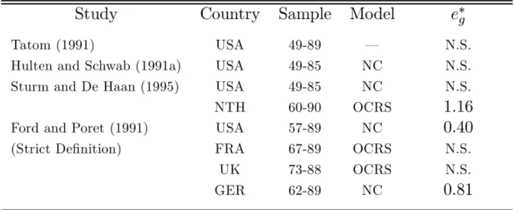
In the same time, we observe that the use of di¤erentiated data (see table 2), justi…ed in the case of non-stationary and not cointegrated series, generally leads to reject the hypothesis of positive e¤ects of the public infrastructures on the productivity of private factors (Tatom 1991, Sturm and De Haan 1995). Thus, the use of this speci…cation seems to clearly indicate that there are important biases in Aschauer’s estimates. This result is not surprising in itself, however the correction proposed in these studies do not allow to con…rm the presence of any productive e¤ects of infrastructures, and this conclusion is more surprising. As Munnell (1992) suggested it, …rst di¤erencing does not constitute in this case the suitable method of stationarization, since it destroys all long term relations which can exist between the variables of interest.

Table 2: Main Emprirical Results: Speci…cations in First Di¤erences Study Country Sample Model e¤g

Tatom (1991) USA 49-89 — N.S.

Hulten and Schwab (1991a) USA 49-85 NC N.S. Sturm and De Haan (1995) USA 49-85 NC N.S.

NTH 60-90 OCRS 1:16

Ford and Poret (1991) USA 57-89 NC 0:40

(Strict De…nition) FRA 67-89 OCRS N.S.

UK 73-88 OCRS N.S.

GER 62-89 NC 0:81

¤_{M o de l: N C : N o C o nstraint, O C R S: O verall C o n stant R etu rn s to Sc ale, N S: N o n S ig ni… ca nt a t 5 %}

These observations lead us to call the speci…cation of the production function in question. If the production function is a cointegrating relation, thus the total factors productivity (TFP) is, by de…nition, covariance stationary. However, nothing makes it possible to a¢rm a priori, that the component of Solow residual orthogonal to public infrastructures, can be represented as a stationary process, contrary to most of macro-economic series. On the contrary, the canonical models of stochastic growth derived from King, Plosser and Rebelo (1988), typically attribute the non stationarity of the economy to the exogenous process of the Solow’s residual. In these models, the cointe-gration between inputs and outputs results from the property of balanced growth and does not coincide with the production function. Besides, from the empirical point of view, the function of production may be represented as a cointegrating relation only if it well speci…ed and it explicitly integrates all the potential explanatory variables of the total productivity, like human capital or education, research and development, measurements of organizational capital, etc.. Then, the omission of one or more of these factors can consequently lead to a fallacious measurement of the Solow’s residual

(8)

and thus harm the identi…cation of a cointegrating relation in the production function. Consequently, some authors, like Crowder and Himarios (1997), are convinced that the production function can not be represented as a long term relation which relates low frequency components of the variables of interest. For them, it is, on the con-trary, a technological constraint which, date by date, relates the high and intermediate frequencies components of these variables.

However, the rejection of the stationarity hypothesis of the total factors productiv-ity does not necessarily imply the absence of any cointegrating relations between the variables of the production function. Particularly, Crowder and Himarios show that American postwar data satisfy the main long run implications of the stochastic bal-anced growth models. In their study, the tests of cointegration hypothesis show1 _that

the output, the stocks of private and public capital, share the same common stochastic trend on the period. The existence of these long term relations, present in particular between the regressors of the equations estimated by Aschauer (1989), can thus lead to an over-estimate of the public infrastructures elasticity. Conversely, the speci…cation in …rst di¤erences can constitute a too ”radical” method (Munnell 1992) which too frequently leads to accept at wrong the null hypothesis eg = 0; since it does not take

into account the long term relations of the system.

Then, in order to analyze more precisely these issues, we now propose a replication of these estimating methods on pseudo samples generated from a theoretical model. This model, used as a data generating process in our exercise, is built so fas to reproduce the main long run relationships observed on postwar American data between the variables of the production function.

3 The data generating process

In order to assess the magnitude of bias in reported estimates of the implicit rate of return on public capital, we consider a stochastic growth model with public capital and a growing total productivity of private factors.

3.1 The model

Let us consider a single good economy, composed by an in…nitely lived representative agent who maximizes the following lifetime expected utility under his budget constraint

max fCt;Ntg1t=0 U = E0 "₁ X t=0 ¯tlog³Ct¡ BAtNt¸ ´# (1)

(9)

where Ct and Nt respectively denote consumption and labor at time t; and ¯ 2 ]0; 1[

is a discount factor. The parameter ¸, with ¸ > 1; controls for the wage elasticity of the labor supply. The parameter B is a scale parameter which determines the marginal disutility of labor (B > 0)2_{. The budget constraint is the following, 8t ¸ 0 :}

Ct+ It· (1 ¡ ¿) wtNt+ (1¡ ¿) rtKt+ (1¡ ¿) ¼t

where wt; rt and ¼t respectively denote real wage, real interest rate and pro…ts.

The production Yt is determined by the levels of private inputs, capital Kt and

labor Nt. The stock of public capital Kg;t is taken as given by the …rm and is assumed

to exert a positive externality on the private factors productivity (Barro 1990). The production function is de…ned by:

Yt= A1t¡ek¡egNtenKtekK eg

g;t (2)

with 8 (ek; eg)2 ]0; 1[2; ek+ eg < 1 and en = 1¡ ek. We assume that the total factor

productivity, denoted At;follows a Random Walk process.

log (At) = log (At¡1) + ²a;t 8t ¸ 1

where A0 > 0 is given and where the innovations ²a;tare i:i:d: (0; ¾2²a): So, in this model,

all growing variables are non stationary. The exogenous factor of growth is determined by the component of Solow’s residual which is orthogonal to the public services. Implicit in this speci…cation is that the aggregate production function, extended to the public capital, can not be speci…ed as a long run relationship. This hypothesis corresponds to the empirical …ndings generally obtained on US postwar data. Finally, we consider log-linear3 _{laws of accumulation for both kinds of capital (Hercowitz and Sampson}

1991).

Kt+1= AkKt1¡±kIt±k Ak > 0 ±k2 ]0; 1[ (3)

Given the aim of our exercise, the only constraint on the theoretical model concerns its stochastic dimension. Indeed, as we will see later, it is necessary to introduce at least as much exogenous shocks in the theoretical model as stochastic regressors used in the empirical models, in order avoid multicolinearity. Given that the estimation of

2_{This speci…cation of preferences implies that the choices of consumption and leisure are not}

in-dependent. Consequently, in order to obtain a balanced growth path, the marginal disutility of labor must grow at the same rate as the marginal utility of consumption. Such a condition is satis…ed when the disutility of labor is augmented by a term At; which is proportional to the factor of growth, as we

will see later.

3_{This hypothesis allows us to obtain analytical rules of decisions at the equilibrium with a strictly}

(10)

a production function with public capital requires to consider at least two stochastic regressors, the data generating process of our pseudo samples must contain at least two stochastic components. Consequently, we assume that public investments are a¤ected by a speci…c shock of productivity4_{, speci…ed as in Greenwood, Hercowitz and Hu¤man}

(1988). As for the private capital, we consider a log-linear speci…cation of the law of accumulation of public capital:

Kg;t+1= AgKg;t1¡±g(Ig;tVg;t)±g (4)

with Ag > 0, ±g 2 ]0; 1[ and where Vg;tdenotes the speci…c shock on public investments.

This shock is assumed to follow a stationary AR (1) process: log (Vg;t) = ½glog (Vg;t¡1) +¡1¡ ½g ¢ log¡Vg ¢ + ²g;t 8t ¸ 1 with Vg;0> 0, ¯

¯½_g¯¯ < 1 and where Vgdenotes the unconditional mean of the process. We

assume here that Vg = 1: The innovations ²g;t are i:i:d:(0; ¾2g); and may be correlated

to the innovations ²a;t: As in Barro (1990), Futagami and alii. (1993), Glomm and

Ravikumar (1997), we assume that public investments are completely …nanced by a proportional and constant tax on revenues, Ig;t= ¿ Yt with ¿ 2 ]0; 1[ :

3.2 Dynamics of the production function variables

In this section, we characterize the dynamics of the production function variables which will be used later to derive the asymptotic distributions of the standard estimators of the public capital elasticity. Given the functional forms of the model, this characterization can be done analytically (see appendix A.1). If we note in upper cases the logarithm, we get 8t > 0: yt= by + ¸ek ¸¡ 1 + ek kt+ ¸eg ¸¡ 1 + ek kg;t+ ¸ (1¡ ek¡ eg)¡ (1 ¡ ek) ¸¡ 1 + ek at (5) kt = bk+ · 1 + ±k¸ (ek¡ 1) + 1 ¡ ek ¸¡ 1 + ek ¸ kt¡1+_¸_{¡ 1 + e}±k¸eg k kg;t¡1 +±k · ¸ (1¡ ek¡ eg)¡ (1 ¡ ek) ¸¡ 1 + ek ¸ at¡1 (6) kg;t = bg+ ±g¸ek ¸¡ 1 + ekkt¡1+ · 1 + ±g¸ (eg¡ 1) + 1 ¡ ek ¸¡ 1 + ek ¸ kg;t¡1 +±g · ¸ (1¡ ek¡ eg)¡ (1 ¡ ek) ¸¡ 1 + ek ¸ at¡1+ ±gvg;t¡1 (7)

4_{This hypothesis can be justi…ed by the uncertainty on the rate of return of the great public}

(11)

nt= bn+ ek ¸¡ 1 + ek kt+ eg ¸¡ 1 + ek kg;t¡ [ek+ eg] ¸¡ 1 + ek at (8)

where by; bk; bg and bn are constants and where the exogenous processes at and vtare

respectively de…ned by at= at¡1+ ²a;t and vg;t= bv+ ½gvg;t¡1+ ²g;t:

4 Stationarity, cointegrating relations and Wold’s

repre-sentations

If we consider this theoretical model as a data generating process, it is now necessary to study the stationary properties of our variables and to identify the cointegrating relations. We show that all factors, except employment, are integrated processes and there exists a fundamental cointegrating relation between private and public capital stocks. All the remainder cointegrated vectors can be deduced from this relationship.

4.1 Stationarity and cointegrating relations

Let us consider the following V ARIMA representation of the vectorial process xt =

(ktkg;t)0:

A (L) (1¡ L) xt= B (L) "t (9)

where ²t= (²a;t²g;t)0 and L denotes the lag operator. Given equations (6) and (7), we

can express the polynomials matrix A (L) and B (L) as following:

A (L) = 0 B @ 1¡ (1 + µk) L ¡_eeg_k (µk+ ±k) L ¡ek eg (µg+ ±g) L 1¡ (1 + µg) L 1 C A (10) B (L) = 0 B B @ ¡hµk ³ eg ek + 1 ´ + ±ke_eg_k i L 0 ¡hµg ³ ek eg + 1 ´ + ±ge_ek_g i L ±gL (1¡ L) ¡ 1¡ ½gL ¢_¡1 1 C C A (11) where µk and µg are two negative constants5, 8¸ > 1:

µk= ±k · ¸ (ek¡ 1) + 1 ¡ ek ¸¡ 1 + ek ¸ (12) µg = ±g · ¸ (eg¡ 1) + 1 ¡ ek ¸¡ 1 + ek ¸ (13)

5_{Given the de…nition of µ}

k and µg; we verify that, if ¸ > 1; µk < 0 and µg < 0 if ¸ >

(1¡ ek) = (1¡ eg) : So, under the hypothesis ek > eg; the constraint ¸ > 1 assure that polynomials

(12)

4.1.1 Stationarity

In this model, the integrated component is induced by the non stationarity hypothesis made on the total factor productivity at:Given the balanced growth property, the non

stationarity of at leads to the presence of an unit root in the dynamics of both stocks

of capital. Then, in the V ARIMA representation (9), we must identify the conditions on structural parameters which ensure the stability of the polynomial A (:) ; since this autoregressive component controls for the dynamics of the growth rates of the capital stocks.

Proposition 1 Denoting (¸1; ¸2) 2 C2 the roots of the polynomial det A (L). The

process associated with the growth rates of private and public stocks of capital is covari-ance stationary (j¸ij > 1; 8i = 1; 2) if and only if the inverse of the wage elasticity of

labor supply satis…es the following condition: ¸ > 1¡ ek

1¡ ek¡ eg (14)

The proof of this proposition is reported in appendix A.2. Under the condition of the proposition 1, the application of the Wold’s (1954) theorem to the process (1 ¡ L) xt

yields the following V MA (1) representation: (1¡ L) xt= " A¤(L) B (L) ¡ 1¡ ¸¡11 L ¢ ¡ 1¡ ¸¡12 L ¢ # "t= H (L) ²t (15) with A¤_{(L) A (L) = det A (L) =}¡₁_{¡ ¸}¡1 1 L ¢ ¡ 1¡ ¸¡12 L ¢

and where the roots of det A (L), denoted ¸i;satisfy j¸ij > 1; 8i = 1; 2: The corresponding polynomial matrix H (L) =

[Hk(L) Hg(L)]0 is: Hk(L) = L det A (L) 0 B @ eg ekªg(µk+ ±k) L + ªk[1¡ (1 + µg) L] eg ek±g(µk+ ±k) L (1¡L) (1¡½gL) 1 C A 0 (16) Hg(L) = L det A (L) 0 B @ ek egªk(µg+ ±g) L + ªg[1¡ (1 + µk) L] ±g[1¡ (1 + µk) L]₍₁(1_¡½¡L) gL) 1 C A 0 (17) where ªkand ªg denote two negative constants6, corresponding to linear combinations

of the parameters µk and µg.

ªk=¡µk µ eg ek + 1 ¶ ¡ ±keg ek ªg =¡µg µ ek eg + 1 ¶ ¡ ±gek eg

6_{Given the de…nition of µ}

k and µg; we show that ªk < 0 and ªg < 0; as soon as ¸ >

(13)

4.1.2 Cointegrating relations

Under the conditions of proposition 1, public and private capital stocks are cointegrated if H (1) is a singular matrix. Given the de…nition of Hg(L) and Hk(L), we get:

Hk(1) = Hg(1) =¡ 1 0 ¢ (18)

Then, the normalized cointegrated vector is given by a basis of the kernel of the linear application H (1) and corresponds to (1; ¡1) : All the remainder cointegrating relations of our model can be deduced from this relation. Particularly, we show that private and public capital stocks are both cointegrated with the total factor productivity at:This property is related to the balanced growth hypothesis of the theoretical model.

In the same way, we can demonstrate that the employment level nt is a stationary

variable, since it can be expressed as a linear function of the stationary processes fkt¡ atg and fkg;t¡ atg (cf. equation 8). Therefore, we get the following long run

properties:

Proposition 2 For this data generating process, the processes fntg and fvg;tg are

covariance stationary, whereas the processes fytg ; fktg ; fkg;tg and fatg are integrated

of order 1 and share the same common trend determined by at:

Then, the main long term properties of this simple balanced growth model are con-sistent with the American historical observations previously mentioned. Most of the empirical studies, devoted to public infrastructures, have concluded to the rejection of the cointegration hypothesis between output and inputs (Aaron 1990, Tatom 1991, Munnell 1992, Sturm and De Haan 1995, Otto and Voss 1997, Sturm 1998). These re-sults imply that the component of the Solow’s residual, which is orthogonal to the public infrastructures productivity e¤ects, is a non stationary process. Besides, Crowder and Himarios (1997) showed that, on postwar US data, private capital, public capital and output share the same common trend and are cointegrated with vector (1; ¡1).

In this context, it is particularly interesting to note that the cointegrated vectors of the model do not reveal any information on the rates of returns of public or private factors. More generally, the estimated cointegrating relations may contain no direct information about structural parameters, and particularly about the technology of pro-duction. It implies that such information may be deduced only from short run or high frequencies ‡uctuations. These preliminary conclusions are similar to those obtained in an other context by Soderlind and Vredin (1996), from a monetary business cy-cle model, where the authors studied the cointegrating relationships between money, output, prices and interest rates.

(14)

4.2 Wold’s decompositions

In order to derive the asymptotic distributions of the empirical moments of the pro-duction function variables, we now establish the Wold decompositions associated to the process f¢ytg ; fntg ; f¢ktg and fkg;tg. The two last are given by equation (16)

and (17). As far as the output is concerned, we …rst notice from equation (5) that the output growth rate dynamics can be expressed as a function of the past shocks.

¢yt= ¸ ¸¡ 1 + ek £ ek eg ¤H (L) ²t+¸ (1¡ ek¡ eg)¡ (1 ¡ ek) ¸¡ 1 + ek ²a;t 1¡ L

From this equation we can derive the V MA (1) representation of the process f¢ytg,

given by ¢yt= Hy(L) ²t with

Hy(L) = µ ¸ ¸¡ 1 + ek ¶ · L det A (L) ¸ £ (19) 0 B B B @ egªg[1¡ (1 ¡ ±k) L] + ekªk[1¡ (1 ¡ ±g) L] + [¸ (1¡ ek¡ eg)¡ (1 ¡ ek)] det A (L) (¸ L)¡1 eg±g[1¡ (1 ¡ ±k) L]₍₁(1_¡½¡L) gL) 1 C C C A 0

As previously mentioned, the employment dynamics only depends on the stationary processes fkt¡ atg and fkg;t¡ atg (cf. equation 8). Since the common trend of both

capital stocks is determined by at, the V MA (1) representation of the process fntg

depends on the stationary component, denoted eH (L) ; issued from the Beveridge and Nelson’s (1981) decomposition of the polynomial matrix H (L) : Let us denote eH (L) = h e Hk(L) ; eHg(L) i0 : nt= bn+ ek ¸¡ 1 + ek e Hk(L) ²t+ eg ¸¡ 1 + ek e Hg(L) ²t (20) with e H (L) = H (L)¡ H (1) (1¡ L) (21)

Given the de…nition of eH (L) ; we can derive the V M A (1) representation of fntg

as function of the structural parameters of the model as follows:

nt= bn+ Hn(L) ²t (22) with Hn(L) = µ ¸ ¸¡ 1 + ek ¶ · 1 det A (L) ¸ £ (23) 0 @ ¡ (ek + eg) + [ekªk+ egªg¡ (1 ¡ ¸1¡ ¸2) (eg+ ek)] L eg±g(1¡ ±k) L2¡1¡ ½gL ¢¡1 1 A 0

(15)

We can observe from these Wold representations, that all the growing endogenous variables ( yt; ktand kg;t) satis…es an ARIMA (3; 1; 3) process, whereas the employment

veri…es an ARMA (3; 2) :

5 Asymptotic distributions of the estimators of the public

capital elasticity

It arises from the examination of the empirical literature, that the evaluations of the rate of return of public infrastructures, carried out through the direct estimate of a production function on aggregate data, lead to very di¤erent results which are all the more implausible. In particular, empirical results are extremely sensitive to the speci…cation, in level or in …rst di¤erences, of the production function. In order to well understand this empirical puzzle, we now determine the results which one would obtain by the application of these various estimating methods to data resulting from the theoretical model presented in the last sections. Since this model has been designed to reproduce as well as possible the long term relations highlighted on American data, this study would allow us to clarify the main stakes evoked in the empirical literature. Besides, given the analytical characterization of the dynamics of the theoretical model, it is possible to establish in this context the exact asymptotic distributions of the various estimators considered.

We limit our analysis to the OLS applied to speci…cations in level or in …rst dif-ferences of the production function, as it is the most commonly used method in the literature. We reduce the study to the two following speci…cations in which the endoge-nous variable is de…ned by the productivity of the stock of private capital yt¡ kt:

yt¡ kt= en(nt¡ kt) + egkg;t+ ¹1;t (24)

yt¡ kt= en(nt¡ kt) + eg(kg;t¡ kt) + ¹2;t (25)

This normalization, used by Aschauer (1989), makes it possible to consider various assumptions on the nature of the scales of returns. The …rst equation (24) corresponds to the assumption of private factors constant returns to scale (P F CRS). This as-sumption is identical to that used in the theoretical model. The second equation (25) corresponds to the assumption of overall constant returns to scale (OCRS). This spec-i…cation corresponds to one of the Aschauers’ specspec-i…cations in which he has obtained a public capital elasticity of 39%, i.e. higher than the estimated private capital elasticity (26%). We now derive the asymptotic distributions of the estimators of the parameters en and eg obtained from the speci…cations (24) and (25).

(16)

5.1 The private factors constant returns to scale (P F CRS)

speci…ca-tion

In the …rst speci…cation (24), the endogenous variable is stationary, and the two sto-chastic regressors follow integrated processes which are cointegrated.

yt¡ kt= en(nt¡ kt) + egkg;t+ ¹1;t (26)

Under the hypothesis bn= 0; we have (cf. appendix A.3):

(nt¡ kt) + kg;t= ©1H (L) ²e t

where the polynomial matrix eH (L) correspond to the stationary component of the Beveridge and Nelson’s decomposition of the process (¢kt ¢kg;t)0 (equation 21) and

where the vector ©1 is de…ned by:

©1= µ 1 ¸¡ 1 + ek ¶_£ (1¡ ¸) ek+ eg¡ 1 + ¸ ¤ (27)

In this case, the two stochastic regressors follow an integrated processes and are cointegrated. According to proposition 2, we know that all the growing variables of the model share the same stochastic common trend. This property implies that empirical moments of all the non-stationary variables converge respectively toward the same asymptotic distribution. Proposition 2 then implies the singularity of the asymptotic variance covariance matrix of the empirical second order moments. Consequently, the derivation of the asymptotic distributions of OLS estimators beg and ben can not be

done directly starting from the speci…cation (26). It is necessary to transform the model before determining these asymptotic distributions.

5.1.1 Triangular representation

We …rst show that it is impossible to derive the asymptotic distributions of OLS esti-mators beg and ben directly starting from the speci…cation (26).

Proposition 3 In the speci…cation (26), the matrix of the empirical second order mo-ments of the vectorial process st= [(nt¡ kt) kg;t]0 converges toward a distribution with

a singular variance covariance matrix.

This proposition is a direct consequence of the proposition 2. Indeed, since the process fnt¡ktg and fkg;tg share the same common stochastic trend, the associated

empirical second order moments converge toward the same distribution (cf. appendix A.3). Consequently, the empirical second order moments of the regressors involved in the construction of the OLS estimator of beg and ben, converges toward a distribution

(17)

characterized by a singular variance covariance matrix. Expressed in other words, this result means that the existence of a common trend, shared by the two stochastic regressors of the speci…cation (26), leads to a degenerated asymptotic distribution of estimators begand ben, since the denominator of these estimators converges7toward zero.

A solution to this problem consists in using a transformation of the speci…cation (26) revealing the residual of the cointegrating relation of the regressors and a non stationary combination of these variables (Park and Phillips 1989).

Proposition 4 The model (26) can be transformed as a triangular representation as following:

yt¡ kt= A0z0;t+ A1z1;t+e¹1;t (28)

with 8i = 0; 1

zi;t= Si0st Ai = ASi (29)

where A = (en eg)0; st= [(nt¡ kt) kg;t]0 and where z0;t and z1;t are two combinations

of the elements of xt which are respectively stationary and integrated of order 1 and

where S = (S0; S1) is an orthogonal matrix.

From this transformed model, it is then possible to determine the asymptotic dis-tribution of estimators ben and beg:The intuition is as follows. If one considers a

trans-formed model including the residual of the cointegrating relation between (nt¡ kt) and

kg;t, the corresponding matrix of variance covariance is non singular. So, the

asymp-totic distributions of the estimators of the parameters of the transformed model can be de…ned. It is then enough to express the parameters of the basic model in the form of combinations of the transformed model parameters. While controlling them by the corresponding speeds of convergence, one …nally obtains the asymptotic distributions of the estimators of the initial model.

The triangular representation of proposition 4 requires to impose some restrictions on S0 and S1. These restrictions correspond to technical assumptions T1.

Assumptions (T1) We assume that the vectors S0 and S1 satisfy the two following

conditions (i) S0S00 + S1S10 = I2 (ii) the vector S0 corresponds to a normalized

basis of the cointegrating space of the process fstg :

7_{In this case, the denominator of these estimators is de…ned by a process which converges towards}

a null punctual mass, in the sense of convergence in probability (p) or in distribution (L). 1 T2 " _T X t=1 (nt¡ kt)2 T X t=1 k2gt¡ T X t=1 (nt¡ kt) kg;t # p =L ¡! T!10

(18)

The …rst condition (i) is necessary to insure the equivalence8 _{between the}

trans-formed model (28) and the initial speci…cation (26). The second condition (ii) imposes that the linear combination z0;t = S00st corresponds, except for a scalar, to the

resid-ual of the cointegrating relation between (nt¡ kt) and kg;t; and is thus stationary by

de…nition. The choice of a normalized basis of the cointegrated space is however not essential, since any monotonous transformation of the cointegrated vector would have allowed us to get representation (28), but it simpli…es calculations. In this model, we immediately get S0 = S1 = 2¡1=2(1 1)0. Under the assumptions (T1), the transformed

model is thus written in the form: yt¡ kt= pA0 2(nt¡ kt+ kg;t) + A1 p 2(nt¡ kt¡ kg;t) + e¹1;t (30) where9 _e¹ 1;t= (en¡ eg) at; z0;t= 2¡1=2(nt¡ kt+ kg;t) ; z1;t= 2¡1=2(nt¡ kt¡ kg;t) and

parameters A0 and A1 are then de…ned by:

A0 = µ en+ eg p 2 ¶ A1= µ en¡ eg p 2 ¶ (31) Given the properties of the speci…cation (30), we can show that the asymptotic distribution of the estimator bA0(which is associated to the residual of the cointegration

relation between the regressors of the initial speci…cation 26) is su¢cient to establish the asymptotic distributions of the estimators bA = (ben beg)0 of the initial parameters.

The intuition is as follows. The bA estimator can be rewritten as: b A = bA0S00 + bA1S10 = bA0S00 + 1 T ³ T bA1S10 ´ = bA0S00 + 1 TOp ¡ T¡1¢ (32) Let us assume that bA0 ¡!L

T!1 eh0 and T bA1 L

¡!

T!1 eh1 where eh0 and eh1 are two non

degenerated distributions with …nite variance, then: b A = µ ben beg ¶ L ¡! T!1eh0S 0 0 (33)

Immediately, given the de…nition of S0, we observe that the estimators ben and

beg converge toward the same asymptotic limit. This result indicates the presence of

a fallacious constraint induced by the cointegrating relation of the regressors. We now characterize eh1;and especially eh0;which enter in the de…nition of the asymptotic

distributions of the transformed estimators bA0 and bA1.

8_{Since, we have:} yt¡ kt= A0z0;t+ A1z1;t+ ¹1;t= A ¡ S0S00 + S1S10 ¢ st+ ¹1;t= Ast+ ¹1;t 9_{The residual e¹}

1;tis a non stationary, but is cointegrated with the I (1) explicative variable; since:

A1 p 2(nt¡ kt¡ kg;t) +e¹1;t= ³ en¡ eg 2 ´ [nt¡ (kt¡ at)¡ (kg;t¡ at)]

(19)

5.1.2 Asymptotic distributions of the estimators beg and ben

From the triangular representation (30), we now derive the asymptotic distributions of the estimators of A0 and A1: We prove in appendix (A.4) that the estimator bA0

converges in distribution toward a punctual mass which corresponds to the correlation between z0;t= 2¡1=2(nt¡ kt+ kg;t) and (yt¡ kt) : The estimator bA1 converges (at the

speed T ) toward a distribution of …nite variance: Then, we get the following results: b A0 p ¡! T!1 E [z0;t(yt¡ kt)] E³z2 0;t ´ (34) T bA1 ¡!L T!1 E [z0;t(yt¡ kt)] eª1¡ E ¡ z0;t2 ¢ eª0 p 2E³z2 0;t ´ ¾2 a 1 R 0 W2 1 (r) dr (35)

where the stochastic variables eª0 and eª1 are de…ned by:

e ª0= Hg(1) P 8 < : 1 Z 0 f W (r)hW (r)f i0dr 9 = ;P0H (1)e 0©00+ 1 X v=0 E [¢kg;t(yt¡v¡ kt¡v)] e ª1 = Hg(1) P 8 < : 1 Z 0 f W (r)hfW (r)i0dr 9 = ;P0H (1)e 0©01+ 1 X v=0 E (¢kg;tz0;t¡v)

where fW (:) = [W1(:) W2(:)]0 denotes a standard Brownian vectorial motion with

E ("t"0t) = - = P P0: The vector ©1 has been previously de…ned (equation 27) and

©0 is: ©0 = µ 1 ¸¡ 1 + ek ¶_£ (1¡ ek) (1¡ ¸) ¸eg ¤ (36)

Given the distributions obtained from the transformed model, we can derive the distributions of the estimators benand beg corresponding to the initial speci…cation (26).

As it was previously mentioned, under assumptions (T1), it is possible to rewrite the estimators ben and beg as linear combinations of bA0 and bA1 (equation 32). Then, we get:

µ ben beg ¶ p ¡! T!1 E [z0;t(yt¡ kt)] E³z2 0;t ´ S₀0 = E [z0;t(yt¡ kt)] E³z2 0;t ´ Ã ₁ p 2 1 p 2 !

Given the de…nition of the transformed variable z0;t; we immediately get the

(20)

Proposition 5 The asymptotic distribution of the OLS estimator of the public capital elasticity eg obtained from the speci…cation (26) is identical to those obtained under the

constraint eg= en: beg p ¡! T!1 E [(yt¡ kt) (nt+ kg;t¡ kt)] E [nt+ kg;t¡ kt]2 (37) Correspondingly: ben ¡!p T!1 E [(yt¡ kt) (nt+ kg;t¡ kt)] E [nt+ kg;t¡ kt]2 (38)

Thus, the application of the OLS on the speci…cation in level (26) leads to impose a fallacious constraint on the parameters of the model. This constraint implies that the elasticities of public capital and employment are asymptotically identical. This result comes from the presence of a cointegrating relation between the non-stationary regres-sors fnt¡ ktg and fkg;tg : Intuitively, in the speci…cation (26), the minimization of the

variance of the residuals imposes that the right member of the equation is homogenous in degree 0 in the I (1) terms. This condition is satis…ed only if en= eg:

Besides, this constraint makes impossible the identi…cation of the elasticity of the public capital. Thus in this exercise, the asymptotic limit of the estimator beg cannot

be expressed in an additive form as a simple function of the true value of the elasticity of the public capital and a term of covariance of the innovations, as in the case of a standard endogeneity bias. Indeed, if we consider the de…nition of processes fktg ;

fkg;tg and fyt¡ ktg, we show that:

E [(yt¡ kt) (nt+ kg;t¡ kt)] E [nt+ kg;t¡ kt]2 = µ en+ eg 2 ¶ + ® (en; eg) µ en¡ eg 2 ¶ (39) with ® (en; eg) = Ef(nt+ kg;t¡ kt) [nt¡ (kt¡ at)¡ (kg;t¡ at)]g E [nt+ kg;t¡ kt]2

Then, if en6= eg (or ek+ eg 6= 1), the asymptotic limit of the estimator beg is a non

linear combination of the parameters en and eg;and thus does not make it possible to

identify the true parameter eg.

From the Wold’s decompositions of the processes fyt¡ ktg and fnt+ kg;t¡ ktg, it is

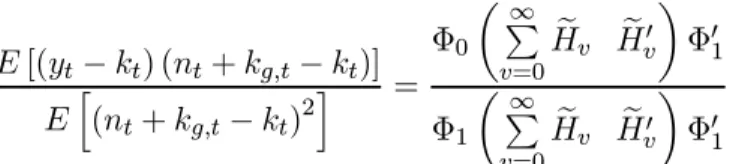
possible to evaluate the correlation (37). For that, we consider the Wold decompositions of these two variables (cf. appendix A.4 ) which are linear functions of the polynomial matrix eH (L). Let us denote eHv the matrix de…ned by eH (L) =P1v=0HevLv. Then, the

(21)

from the following expression: E [(yt¡ kt) (nt+ kg;t¡ kt)] Eh(nt+ kg;t¡ kt)2 i = ©0 µ₁ P v=0 e Hv- eHv0 ¶ ©01 ©1 µ₁ P v=0 e Hv- eHv0 ¶ ©0 1

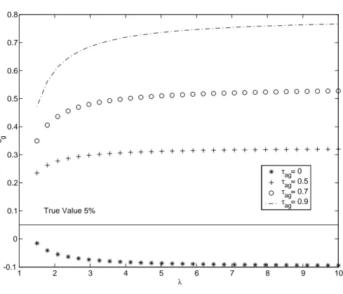
Since this expression is a particularly complicated function of the structural para-meters, we propose on …gure 1 a numerical evaluation of this correlation for various values of the correlation of the shocks ¿ag and of the inverse of the elasticity of labor

supply ¸ (these values satisfy the conditions of proposition 1). In order to compare our results to those of Aschauer (1989), the other structural parameters of the model are calibrated on American data. In particular, the value of the elasticity of the production compared to the stock of public capital is …xed at 5% (represented by a horizontal line on the graph). This value corresponds to the empirical mean of public investment ratio obtained on postwar data (Baxter and King 1993).

Figure 1: Asymptotic Distribution of beg (P F CRS Hypothesis)

1 2 3 4 5 6 7 8 9 10 -0.4 -0.2 0 0.2 0.4 0.6 0.8 1 eg λ Vraie Valeur 5% τ_ag= 0 τ_ag= 0.5 τ_ag= 0.7 τ_ag= 0.9

When the correlation between the two shocks is null or negative, the OLS estimator of begconverges toward a negative quantity. But when this correlation is su¢ciently high,

this quantity becomes positive. One can observe that for values of ¸ higher than the calibrated value of 3:65, the estimator beg tends to largely over-estimate the elasticity

(22)

of public capital. Besides, there are several values of the couple (¸; ¿ag) for which the

OLS estimator converges toward values higher than 40%, identical to those estimated by Aschauer (1989) on US data, whereas the calibrated value of elasticity is only 5% in the theoretical model.

More generally, we may consider that if an asymptotic constraint of type en = eg

exists, then OLS lead to over-estimate the rates of returns of these infrastructures. This fallacious constraint could appear as soon as the two explicative variables share the same common stochastic trend. Such a con…guration is not particular to our problem and could occur in many economic issues (estimates rate of returns on human capital, commercial opening etc..). Besides, it implies that long run relations may be not su¢cient to get information about the structural parameters of the economy (Soderlind and Vredin 1996).

5.2 The overall constant returns to scale (OCRS) speci…cation

The second speci…cation of the production function (40), used notably by Aschauer (1989), corresponds to the hypothesis of overall constant returns to scale (OCRS):

yt¡ kt= en(nt¡ kt) + eg(kg;t¡ kt) + ¹2;t (40)

In this speci…cation, one of the two explicative variables, kg;t¡ kt, is stationary

whereas the second one, nt¡ kt; follows an I (1) process. The residual ¹2;t is non

stationary and is de…ned by ¹_2;t= (en¡ eg) at+ egkt:Then, since ¹2;t is cointegrated

with the regressor nt¡ kt according to a cointegrated vector (1; en) ; the residual

popu-lation can be expressed as the sum of two components respectively stationary and non stationary:

¹_2;t=e¹2;t¡ en(nt¡ kt) (41)

where the stationary process e¹2;t is de…ned by:

e¹2;t= ennt+ (eg¡ en) (kt¡ at) = ©2H (L) "e t (42) with ©2 = h ³ enek ¸¡en ´ + eg¡ en ³_e neg ¸¡en ´ i (43) In the expression (41), the non stationary component of ¹_2;t is proportional to the regressor nt¡ kt: The stationary component e¹2;t corresponds to the residual of the

cointegrating relation between nt¡ kt and ¹2;t. This process is a linear combination

of the elements of polynomial matrix eH (L) issued from the Beveridge and Nelson’s decomposition of (¢kt; ¢kg;t) : Given this decomposition of the residual population, we

will show that the OLS estimator leads to a biased measure of the public capital stock elasticity.

(23)

5.2.1 Asymptotic distributions of beg and ben

Given the cointegrating relation between the residual ¹_2;t and the regressor nt¡ kt;we

can transform the speci…cation (40) as a standard regression where all the explanatory variables are stationary and where the coe¢cient en is not identi…ed.

yt¡ kt= eg(kg;t¡ kt) +e¹2;t

This expression indicates that (i) the estimator begin the speci…cation (40) converges

toward the correlation between the private capital productivity and the ratio kg;t¡ kt

and (ii) the employment elasticity can not be identi…ed, since under H0the term nt¡kt

disappears.

Proposition 6 In the speci…cation (40) of the production function, the OLS estimators of the parameters en and eg are not convergent since:

(i) The OLS estimate of public capital elasticity beg is a¤ected by a standard endogeneity

bias due to the correlation between kg;t¡ kt and the stationary component e¹2;t of the

population residual. beg¡ eg ¡!p T!1 E£(kg;t¡ kt)e¹2;t ¤ Eh(kg;t¡ kt)2 i (44)

(ii) The OLS estimate of labor elasticity ben converges toward 0 since:

Tben ¡!L T!1 Eh(kg;t¡ kt)2 i e ª2¡ E£(kg;t¡ kt)e¹2;t¤ eª3 Eh(kg;t¡ kt)2 i ¾2 a 1 R 0 W2 1 (r) dr (45)

where the stochastic variables eª2 and eª3 are respectively de…ned by

e ª2 =¡Hg(1) P 8 < : 1 Z 0 f W (r)hfW (r)i0dr 9 = ;P0H (1)e 0_©0 2+ 1 X v=0 E£¢ (nt¡ kt)e¹_2;t¡v¤ e ª3=¡Hg(1) P 8 < : 1 Z 0 f W (r)hW (r)f i0dr 9 = ;P0H (1)e 0_©0 3+ 1 X v=0 E [¢ (nt¡ kt) (kg;t¡v¡ kt¡v)] with ©3 =£ ¡1 1 ¤0 and ©2 = h ³ enek ¸¡en ´ + eg¡ en ³_e neg ¸¡en ´ i0 :

The proof of the proposition 6 is provided in appendix A.5. These results clearly in-dicate that the application of OLS on a speci…cation in level of the production function under the OCRS hypothesis leads to a biased estimates of the public capital elastic-ity and to an undervaluation of the labor elasticelastic-ity (since the corresponding estimator converges toward 0).

(24)

It is important to remind that it is precisely this methodology that has been used in many empirical studies devoted to the measure of the public capital rates of returns and notably in Aschauer (1989). From an identical speci…cation to (40), Aschauer put in obviousness a very high and signi…cant estimated elasticity of the public capital (39%), while the estimated labor elasticity (35%) was largely inferior to those generally estimated in two factors production functions (where one generally …nds a contribution of labor around 2=3). These observations are compatible with the conclusions of the proposition 6.

Of course, we can not generalize these observations, since all our asymptotic re-sults are conditional to the speci…cations of our theoretical DGP . However, we can a¢rm here, that if historical American data are generated by a process similar to the V ARIMAprocess exposed below and satisfy the long run implications of a balanced growth model, the use of OLS on the speci…cation (40) leads to a biased measure of the public capital implicit rate of returns. Since, these conditions are not very restrictive, there is a great probability that the corresponding empirical results may be biased and not well founded. We now propose a numerical evaluations of these asymptotic biases for reasonable values of the structural parameters.

5.2.2 Evaluation of the bias on beg

As in the P F CRS case, we now derive the asymptotic limit of the estimator beg as a

linear function of the stationary components of the Beveridge and Nelson’s decompo-sition of (¢kt¢kg;t)0: By developing the expression of the stationary component e¹2;t;

we can rewrite the bias on beg as following:

beg¡ eg p ¡! T!1(1¡ ek¡ eg) E [(kg;t¡ kt) (at¡ kt)] Eh(kg;t¡ kt)2 i + (1¡ ek)E [(kg;t¡ kt) nt] Eh(kg;t¡ kt)2 i where the variables (kg;t¡ kt) = ©3H (L) ²e t and e¹2;t = ©2H (L) ²e t are linear

com-binations of the stationary components eH (L) ²t. From these two relations and the

covariance matrix of Zt = eH (L) ²t; it is possible to calculate numerically the value of

the asymptotic bias:

As in the case of the speci…cation (24), the values of this correlation are plotted for di¤erent values of ¸ and ¿ag on the …gure 2. The other structural parameters are

(25)

Figure 2: Asymptotic Distribution of beg (OCRS Hypothesis) 1 2 3 4 5 6 7 8 9 10 -0.1 0 0.1 0.2 0.3 0.4 0.5 0.6 0.7 0.8 eg λ τ_ag= 0 τ_ag= 0.5 τ_ag= 0.7 τ_ag= 0.9 True Value 5%

For a positive correlation between the two shocks, we can observe that the endo-geneity bias leads to largely over-estimate the value of the public capital elasticity. For values of ¸ superior to the calibrated value of 3:65, the estimated elasticity is thus be-tween 28% and 80%, whereas the true value is only 5%. However, when the two shocks are independent, the utility speci…cation (particularly the absence of wealth e¤ects in the labor supply) leads to a negative correlation between the ratio kg;t¡ kt and the

stationary component of the population residual e¹2;t:Then, the OLS estimator

under-evaluate the true value of the elasticity (5%). This result can be explained by the fact that in this case, the employment level, which enters in the de…nition of the residual e¹2;t, is negatively correlated to the ratio kg;t¡ kt. An increase in the public capital

stock implies an improvement of the private inputs productivity that incites the agent to substitute future labor to present labor.

6 Finite samples properties

As it was mentioned previously, the use of di¤erentiated data (justi…ed in the case of non-stationary and not cointegrated series) generally leads to reject the hypothesis of positive e¤ects of the public infrastructures on the productivity of private factors. We

(26)

propose here to replicate this speci…cation on …nite pseudo samples issued from our theoretical model. We consider 10 000 Monte Carlo pseudo samples, of size T = 50; which is roughly the average size of annual samples used in the empirical literature (cf. table 1). The structural parameters are calibrated as in section 4. In particular, the public capital elasticity eg is set to 5%. The parameter ¸ is …xed to 3:65, which implied

an elasticity of labor of 37% (Hercowitz 1986).

Let us consider the two following models under P F CRS and OCRC hypothesis 8s = 1; :; S: ¢yes_t(µ)¡ ¢ekst(µ) =besn h ¢enst(µ)¡ ¢ekst(µ) i +besg¢eksg;t(µ) +b¹s1;t (47) ¢eyst(µ)¡ ¢ekst(µ) =besn h ¢enst(µ)¡ ¢ekst(µ) i +besg h ¢ekg;ts (µ)¡ ¢ekts(µ) i +b¹s1;t (48) where ezs

t(µ) ; z =fk; kg; yg ; denotes a sample of the endogenous variables issued from

a simulation s, with s 2 [1; S], realized conditionally to a value µ of the set of structural parameters and conditionally to a particular realization of structural shocks.

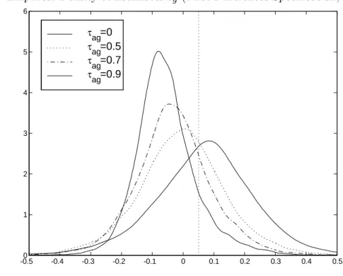
Figure 3: Empirical Density of Estimates beg (First Di¤erences Speci…cation, P F CRS)

-0.50 -0.4 -0.3 -0.2 -0.1 0 0.1 0.2 0.3 0.4 0.5 1 2 3 4 5 6 τ_ag=0 τ_ag=0.5 τ_ag=0.7 τ_ag=0.9

The …gure (3) reproduces the empirical distribution of the estimates bes

g get from

the equation (47), for di¤erent values of the correlation ¿a;g of shocks. We can observe

(27)

of the public capital elasticity. However, the range of the bias is largely inferior to the bias observed on level speci…cations. Given the hypothesis on ¿a;g, the empirical mean

of estimates lies between ¡0:3% and ¡5%:

The use of …rst di¤erentiated data has also implications on the results of inference tests. Indeed, as we can observe on table 3, …rst di¤erencing leads too frequently to accept at wrong the null hypothesis bes

g = 0: In this table, the empirical frequencies

(from 10 000 pseudo samples) of the rejection of the null hypothesis bes

g = 0; at the

traditional level of 5% are reproduced.

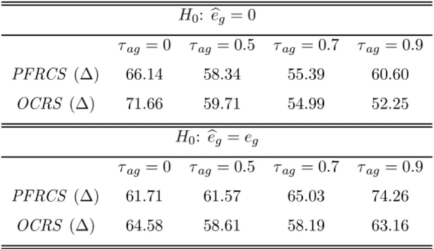
Table 3: Empirical Frequencies of Rejection of beg = ®

H0: beg= 0 ¿ag = 0 ¿ag = 0:5 ¿ag= 0:7 ¿ag = 0:9 PFRCS (¢) 66.14 58.34 55.39 60.60 OCRS (¢) 71.66 59.71 54.99 52.25 H0: beg = eg ¿ag = 0 ¿ag = 0:5 ¿ag= 0:7 ¿ag = 0:9 PFRCS (¢) 61.71 61.57 65.03 74.26 OCRS (¢) 64.58 58.61 58.19 63.16

The empirical probability to accept at wrong the hypothesis of nullity of public capital elasticity lies between 34% and 45%, given the value of ¿a;g: Indeed, in one

pseudo sample on three, the Student statistic leads to reject at 5% the hypothesis of a productive contribution of public capital, whereas in our model the public capital is one of the inputs of the production function. Besides, the null hypothesis bes

g = eg = 5%

is rejected at wrong in more than 60% of our pseudo samples.

It clearly indicates that …rst di¤erencing the data is not the suitable method of stationarization in our context. These results are not surprising, since we have assumed a common stochastic trend for all variables. The suitable method consists here in applying the Beveridge and Nelson’s decomposition to all growing variables and to consider only deviations from the common stochastic trend. Moreover, …rst di¤erencing the covariance stationary input ntimplies an autocorrelation of residuals and then non

standard asymptotic distributions for the Student statistics. As it was suggested by Munnell (1992), …rst di¤erencing may be too ”radical” since it destroys all the long term relations of the variables of the production function.

(28)

7 Conclusion

This exercise shows that the production function approach (applied to times series at least), commonly used in econometric studies, does not provide a reliable inference strategy and may not be the best way to determine the genuine rate of return of public infrastructures. Indeed, given a data generating process built so as to match the main long term properties of production function variables, we prove here that two main sources of bias could a¤ect the estimates of the public capital elasticity. First, there may be a standard endogeneity bias due to the simultaneous determination of private and public inputs. The second source of bias is more original and comes from the presence of a common stochastic trend shared by all non stationary inputs. In this case, we show that there is a fallacious asymptotic constraint which imposes the equality between the public capital elasticity and the labor one. In both cases, the production function approach, applied on speci…cations in level could largely over-estimate the macroeconomic returns of infrastructures. Besides, given the long term properties of the model, the traditional correction based on a speci…cation in …rst di¤erences could lead to a fallacious inference. In particular, it induces a too frequently rejection at wrong of the null hypothesis of a positive productive contribution of infrastructures.

These conclusions imply that cointegration relations may contain no direct informa-tion about structural parameters of the producinforma-tion funcinforma-tion, but that such informainforma-tion may be deduced from short-run or high frequencies ‡uctuations. Consequently, it is necessary to precisely identify the common stochastic trends of the production function variables, in order to obtain short run ‡uctuations of these variables. In other words, it is necessary to give up the partial equilibrium approach, generally used in the empirical literature, and to adopt a more structural or theoretical approach. Several technical solutions could be adopted. The …rst, consists in estimating the common trends and to evaluating the productive contribution of infrastructures only with the deviations of data from these trends. The second kind of solutions is to directly estimate the structural model with indirect inference methods for instance. The conclusions of this exercise may be transposed to several other bodies of applied researches. The study of the macroeconomic productive contribution of human capital is one of them.

(29)

A Appendix

A.1 Dynamics of the production function variables

In this model, we consider the public decisions path fKg;t; Ig;tg1_t=0 as given and we

determine the equilibrium conditionally to this path. The program is: max fCt;Nt;Kt+1g1t=0 E0 1 X t=0 ¯tlog³Ct¡ BAtNt¸ ´ (49) under (1 ¡ ¿) A1¡ek¡eg

t Nt1¡ekKtekK eg g;t= Ct+ A ¡1 ±k k K 1 ±k t+1K ±k¡1 ±k t

Ex-post, the public capital stock path is determined by the relation Kg;t+1 =

AgKg;t1¡±g(¿ YtVg;t)±g:The solution of the program (49) veri…es the Bellman’s equation

for an optimal path of private capital: V (Kt; Kg;t; At; Vg;t) = max fCt;Nt;Kt+1gfU (C t; Nt) + ¯EtV (Kt+1; Kg;t+1; At+1; Vg;t+1)g with Kt+1 = AkKt1¡±k h (1¡ ¿) A1¡ek¡eg t Nt1¡ekKtekK eg g;t¡ Ct i±k

and with transversality condition: lim t!1¯ t_E 0 ½ @V (St+1) @Kt+1 Kt ¾ = 0

This program is resolved by the method of undetermined coe¢cients. Given the log-linear speci…cation of the model, we guess a log-linear form to the value function V (:) given by:

V (:) = V0+ V1log (Kt) + V2log (Kg;t) + V3log (At) + V4log (Vg;t)

By substitution of the derivative @V (:) =@K in the …rst order conditions of the representative agent’s program, we obtain the private investment ratio and the saving rate, denoted s: The saving rate is constant and implies a unity correlation between production and investment. This restriction is due to the log-linear speci…cation of the model. It= A ¡1 ±k k K 1 ±k t+1K ±k¡1 ±k t = s (1¡ ¿) Yt Ct= (1¡ ¿) (1 ¡ s) Yt

with s = (¯ek±k) = [1¡ ¯ (1 ¡ ±k)] > 0; since ¯ < 1: By substituting these expressions in

the …rst order conditions of the program, we get (8), (5), (6) and (7). The corresponding constant terms are :

bn= 1

¸¡ 1 + ek

[log (1¡ ¿) + log (1 ¡ ek)¡ log (B) ¡ log (¸)]

by = (1¡ ek) bn

bk= log (Ak) + ±k[log (s) + by+ log (1¡ ¿)]

(30)

A.2 Stability conditions of A (L)

We consider the polynomial of order two det [A (L)] = 1 + aL + bL2 _{where a =}

¡ (2 + µk+ µg) and b = (1 + µk) (1 + µg)¡ (µk+ ±k) (µg+ ±g) : The roots of the A (L)

are noted ¸i 2 C, 8i = 1; 2: Three constraints on the parameters a and b insure that

the roots of A (L) are outside the unit circle in modulus:

b < 1 1 + a + b > 0 1¡ a + b > 0

Given the de…nition of µkand µg(equations 12 and 13), under the hypothesis ¸ > 1;

we can rewrite these conditions as combinations of structural parameters as following: ¸ > Ã1= (1¡ ek) (±k+ ±g¡ ±k±g) (1¡ ek) ±k(1¡ ±g) + (1¡ eg) ±g(1¡ ±k) + ±k±g (50) ¸ > Ã₂ = 1¡ ek 1¡ ek¡ eg (51) ¸ > Ã₃ = (1¡ ek) [2 (2¡ ±k¡ ±g) + ±k±g] ek±k(1¡ ±g) + eg±g(1¡ ±k) + 2 (2¡ ±k¡ ±g) + ±k±g (52)

Under the hypothesis ¸ > 1; the third condition (52) is always satisfy as soon as the depreciation rates are inferior to one (±k < 1 and ±g < 1). The …rst condition (50)

is always satis…ed if ek > eg(1¡ ±k) ; since then Ã1 < 1: In other cases, we have to

compare the thresholds Ã₁ and Ã₂:We show that: Ã1¡ Ã2 =¡

(1¡ ek) (eg±g+ ek±k)

(1¡ ek¡ eg) [(1¡ ek) ±k(1¡ ±g) + (1¡ eg) ±g(1¡ ±k) + ±k±g]

This expression is strictly negative as soon as depreciation rates are inferior to one and e_k + eg < 1: Then, there is only one constraint on the parameter ¸ which insures

that the dynamics of capital growth rates are covariance stationary, that is to say j¸ij > 1; 8i = 1; 2. This constraint corresponds to the thresholds Ã2 and is given in the

proposition (1).

A.3 Asymptotic distributions of empirical second order moments

Let us consider the following de…nition of the polynomial matrix eH (L) : e H (L) "t= [H (L)¡ H (1)] (1¡ L) "t= µ kt¡ at kg;t¡ at ¶

Now, consider the vector st= [(nt¡ kt) kg;t]0:Given, the de…nitions (equations 8,

6 and 7) of the processes fntg ; fktg and fkg;tg we show that:

(31)

h

i₀ : The asymptotic distributions of the corresponding empirical moments are then de…ned by: 1 T2 T X t=1 sts0t ¡!L T!1© (1) P 8 < : 1 Z 0 f W (r)hW (r)f i0dr 9 = ;P0© (1) 0₊ 1 T2Op (T ) (53)

where fW (:) = [W1(:) W2(:)]0 is a standard vectorial Brownian motion. Using the

de…nitions of the polynomial vectors Hk(:) and Hg(:) (equations 16 and 17) we can

verify the singularity of the asymptotic variance covariance matrix of the system: 1 T2 T X t=1 sts0t ¡!L T!1¾ 2 a µ 1 ¡1 ¡1 1 ¶_Z1 0 W1(r)2dr

A.4 Asymptotic distributions under the P F CRS hypothesis

In the transformed model (30), the OLS estimators bA0 and bA1 are the following:

b A0 = T¡2 T P t=1 ¡ z21;t ¢ T¡1 T P t=1 [z0;t(yt¡ kt)]¡¡T¡1¢ T¡1 T P t=1 (z1;tz0;t) T¡1 T P t=1 [z1;t(yt¡ kt)] T¡1 PT t=1 ³ z_0;t2 ´T¡2 PT t=1 ³ z_1;t2 ´¡ · T¡1 PT t=1 (z1;tz0;t) ¸2 (T¡1₎ (54) T bA1= T¡1 T P t=1 ¡ z0;t2 ¢ T¡1 T P t=1[z1;t(yt¡ kt)]¡ T ¡1 PT t=1(z1;tz0;t) T ¡1 PT t=1[z0;t(yt¡ kt)] T¡1 PT t=1 ³ z_0;t2 ´T¡2 PT t=1 ³ z2_1;t´¡ (T¡1₎ · T¡1 PT t=1(z1;tz0;t) ¸2 (55) Given the dynamic properties of the theoretical model, the Wold’s decompositions associated to the processes z0;t; z1;t and to the endogenous variable yt ¡ kt of the

transformed model (30) are de…ned by:

yt¡ kt= ©0H (L) ²e t (56) p 2z0;t = nt¡ kt+ kg;t= ©1H (L) ²e t (57) p 2¢z1;t = ¢ [nt¡ kt¡ kg;t] = z0;t¡ 2kg;t (58) = h(1¡ L) ©1H (L)e ¡ 2Hg(L) i "t

(32)

where ¢kg;t = Hg(L) "t (equation 17) and where the polynomial vector eH (L)

corre-sponds to the stationary component of the Beveridge and Nelson’s decomposition of the process (¢kt¢kg;t)0 (equation 21). The vectors ©0 and ©1 have respectively de…ned

in equations (36) and (27). Then, we can derive the asymptotic distributions of the corresponding empirical moments:

1 T2 T X t=1 z2_1;t = 1 T2 T X t=1 ³ z0;t¡ p 2kg;t ´2 = 2 T2 T X t=1 kg;t2 + 1 TOp (T ) L ¡! T!12¾ 2 a 1 Z 0 W1(r)2dr 1 T T X t=1 [z0;t(yt¡ kt)] ¡!p T!1E [z0;t(yt¡ kt)] 1 T T X t=1 z20;t p ¡! T!1E ¡ z0;t2 ¢ In the same way, we show that:

1 T T X t=1 z0;tz1;t= 1 T T X t=1 z20;t¡ p 21 T T X t=1 z0;tkg;t L ¡! T!1E ¡ z20;t ¢ ¡p2Hg(1) P 8 < : 1 Z 0 f W (r)hW (r)f i0dr 9 = ;P0H (1)e 0_© 1¡ p 2¤1

where fW (:) = [W1(:) W2(:)]0 denotes a standard vectorial Brownian motion and where

E ("t"0t) = - = P P0: The parameter ¤1 is de…ned by ¤1 = P1v=0E (¢kg;tz0;t¡v) :

Finally, we have: 1 T T X t=1 z1;t(yt¡ kt) = 1 T T X t=1 z0;t(yt¡ kt)¡ p 21 T T X t=1 kg;t(yt¡ kt) L ¡! T!1E [z0;t(yt¡ kt)]¡ p 2Hg(1) P 8 < : 1 Z 0 f W (r)hW (r)f i0dr 9 = ;P0H (1)e 0_© 0¡ p 2¤0

where the parameter ¤0 is de…ned by ¤0 = P1v=0E [¢kg;t(yt¡v¡ kt¡v)] : Then, the

asymptotic distribution of bA0 can be immediately derived since:

b A0= T¡2 PT t=1 ¡ z2 1;t ¢ T¡1 PT t=1 [z0;t(yt¡ kt)]¡ T¡3Op ¡ T2¢ T¡1 PT t=1 ³ z2 0;t ´ T¡2 PT t=1 ³ z2 1;t ´ ¡ T¡3_{Op (T}2₎ L ¡! T!1 E [z0;t(yt¡ kt)] E³z_0;t2 ´ (59)

(33)

The estimator bA0 converges in distribution toward a null punctual mass, and this

result ensures the convergence in probability. Given the distributions of the empirical moment, and the de…nition of bA1;(equation 55), we get:

T bA1 ¡!L T!1 E [z0;t(yt¡ kt)] eª1¡ E ¡ z_0;t2 ¢ eª0 p 2E³z2 0;t ´ ¾2 a 1 R 0 W2 1 (r) dr (60)

where the stochastic variables eªj; j = (1; 2) are de…ned by:

A.5 Asymptotic distributions under the OCRS hypothesis

From the expressions of the dynamics of the production function variables, we can derive the Wold’s decomposition associated to the processes fkg;t¡ ktg ; fnt¡ ktg and

fyt¡ ktg. After simple calculations, we obtain the following results.

where the polynomial vector Hg(L) corresponds to the Wold’s decomposition of the

functional central limit and the continuous mapping theorems, we immediately get: 1 T2 T X t=1 (nt¡ kt)2 = 1 T2 T X t=1 k2t + 1 TOp (T ) L ¡! T!14¾ 2 a 1 Z 0 W1(r)2dr (64) 1 T T X t=1 £ (kg;t¡ kt)¹e2;t ¤ p ¡! T!1E £ (kg;t¡ kt)e¹2;t ¤ (65) 1 T T X t=1 (kg;t¡ kt)2 p ¡! T!1E h (kg;t¡ kt)2 i (66) where W1(:) is standard scalar Brownian motion. In the same way, we get:

(34)

1 T T X t=1 (nt¡ kt) (kg;t¡ kt) ¡!L T!1¡Hg(1) P 8 < : 1 Z 0 f W (r)hW (r)f i0dr 9 = ;P0H (1)e 0_©0 3+ ¤3 (68) where E ("t"0t) = - = P P0 and where fW (:) = [W1(:) W2(:)]0 denotes a standard

vectorial Brownian motion, with ¤2 = 1 X v=0 E£¢ (nt¡ kt)e¹2;t¡v ¤ ¤3= 1 X v=0 E [¢ (nt¡ kt) (kg;t¡v¡ kt¡v)]

Then, we transform the expression of the estimator beg in order to control for the

di¤erent speeds of convergence:

beg¡ eg = T P t=1 h (nt¡kt)2 T2 i _PT t=1 h_(k g;t¡kt)e¹2;t T i ¡¡T1 ¢ _PT t=1 h_(n t¡kt)(kg;t¡kt) T i _PT t=1 h_(n t¡kt)e¹2;t T i T P t=1 h (nt¡kt)2 T2 i _PT t=1 h (kgt¡kt)2 T i ¡¡T1 ¢·_PT t=1 (nt¡kt)(kg;t¡kt) T ¸2

Given distributions (64) to (68), we get:

beg¡eg= T P t=1 h (nt¡kt)2 T2 i _PT t=1 h_(k g;t¡kt)e¹2;t T i ¡¡1 T ¢ Op¡T2¢ T P t=1 h (nt¡kt)2 T2 i _PT t=1 h (kgt¡kt)2 T i ¡¡T1 ¢ Op (T2₎ L ¡! T!1 E£(kg;t¡ kt)e¹2;t ¤ Eh(kgt¡ kt)2 i (69) The centered estimator beg ¡ eg converges in distribution toward a punctual mass

corresponding to the correlation between kg;t¡ ktand e¹2;t.

In the same way, it is possible to derive the asymptotic distribution of ben: We

consider the following de…nition:

Tben= T P t=1 h (kg;t¡kt)2 T i _PT t=1 h_(n g;t¡kt)e¹2;t T i ¡ PT t=1 h (nt¡kt)(kg;t¡kt) T i _PT t=1 h_(k g;t¡kt)e¹2;t T i T P t=1 h (nt¡kt)2 T2 i _PT t=1 h (kgt¡kt)2 T i ¡¡_T1¢ ·_T P t=1 (nt¡kt)(kg;t¡kt) T ¸2 We get: Tben ¡!L T!1 Eh(kg;t¡ kt)2 i e ª2¡ E £ (kg;t¡ kt)e¹2;t¤ eª3 Eh(kg;t¡ kt)2 i ¾2 a 1 R 0 W2 1 (r) dr (70)

where the stochastic variables eª2 and eª3 are de…ned by: