Are Public Investment E¢ cient in Creating
Capital Stocks in Developing Countries?
Florence Aresto¤
yand Christophe Hurlin
zSeptember, 2010
Abstract
In many poor countries, the problem is not that governments do not invest, but that these investments do not create productive capital. So, the cost of public investments does not correspond to the value of the capital stocks. In this paper, we propose an original non parametric approach to evaluate the e¢ ciency function that links variations (net of depreciation) of stocks to public investments. We consider four sectors (electricity, telecom-munications, roads and railways) of two Latin American countries (Mexico and Colombia). We show that there is a large discrepancy between the amount of investments and the value of increases in stocks.
Key Words: Public Capital, Capital Stocks, Developing Countries. J.E.L Classi…cation Numbers: C82, E22, E62
1
Introduction
Since the seminal works of Aschauer (1989), the measure of the productivity and the e¢ ciency of infrastructure and public capital has been the subject of many empirical studies, for OECD countries (see the surveys of Gramlich, 1994 or Sturm, 1998) but also for developing countries (World Development Report for 1994, Canning, 1999, or Easterly and Serven, 2004). The traditional method used
This paper has been produced as part of a World Bank research project “The productivity E¤ects of Public Capital in Developing Countries” sponsored by the Powerty Reduction and Economic Management Network (PRM). We thank Santiago Herrera for his support and his comments on a previous version of this work (World Bank Policy Research Working Paper 3858, March 2006).
y1) Université Paris Dauphine, LEDa, 75016 Paris, France 2) IRD, UMR 225-DIAL,
F-75010, Paris, France. E-mail address: ‡orence.aresto¤@dauphine.fr
zLEO, Université d’Orléans. Rue de Blois. BP 6739. 45067 Orléans Cedex 2. France.
to estimate capital stocks for OECD countries is the Perpetual Inventory Method (PIM, thereafter). This well known method consists in cumulating historical series of past investments and in deducting assets which were retired. The PIM has been used to estimate public capital stocks among others by Sturm and De Haan (1995) for the Netherlands,Berndt and Hansson (1992) for Sweden, Ford and Poret (1991) for France and Japan and more recently by Kamps (2004) for as sample of 22 OECD countries. But Pritchett (1996) showed that in many poor countries the problem is not that governments do not invest, but that these investments do not create productive capital. The cost of public investments does not correspond to the value of the capital stocks. Pritchett estimates that only slightly more than half of the money invested in investment projects will have a positive impact on public capital stocks in developing countries.
Consequently, we propose to evaluate the relationship between the increase in monetary value of stocks and the current monetary value of public investments in two developing countries, Colombia and Mexico. This relation, called e¢ ciency function, indicates the value of the public capital produced by one dollar’s worth of government investment spending. If the PIM is valid, we should verify that one invested dollar increases the stock value with one dollar. On the contrary, if it is observed that the stocks value is increased with less than one dollar, it implies that the PIM overvalues the public stocks. Using infrastructure physical measures proposed by Canning (1998), we adopt a non-parametric approach to give an estimate of the portion of public investments that are e¢ cient in creating capital.
The rest of the paper is organized as follows. Section 2 is devoted to the measure of public investment e¢ ciency. Section 3 presents tthe results and section 4 concludes.
2
Public Investment E¢ ciency : Data and
Method-ology
Pritchett (1996) and Canning (1998) state that the same investment ‡ows in di¤erent countries may have very di¤erent e¤ectiveness in actually producing capital, due to the di¤erences in public sector e¢ ciency and di¤erences in the price of capital. If the investment project is carried out by public sector, actual and economic costs (de…ned as the minimum of possible costs given available technology) may deviate. So, the use of monetary investment may introduce systematic errors in the amount of public capital actually produced.
Let us consider the following capital accumulation relationship:
Kt+1= (1 ) Kt+ f (It) (1)
where Kt denotes the public capital stock at time t and I denotes the
represents the e¢ ciency of public investments to generate new capital. If we assume that only a certain part of investments is used to create capital, the func-tion f (:) may di¤er from identity funcfunc-tion. We only know that it satis…es the following constraints:
0 f (It) It (2)
f (0) = 0 (3)
The fact that f (It)can be strictly inferior to It re‡ects the ine¢ ciency of
public investments in creating capital. Since no natural speci…cation of the ef-…ciency function f (:) can be justi…ed a priori, a solution consists in estimating this function by a non parametric method for a typical developing country or for a sub-group of developing countries. For this purpose, three inputs are re-quired: (1) a series of public investments (2) the depreciation rates (or its time pro…le) and (3) a series of public capital stocks e¤ectively available in the refer-ence countries. The …rst and the second element are available in the literature (World Bank, Bureau of Economic Analysis) for many countries. But the last element does not exist. Consequently, in this study, we propose to estimate the e¢ ciency function by using physical measure of infrastructure as a proxy of pub-lic capital stock e¤ectively available in developing countries. To the best of our knowledge, only the Calderon, Easterly and Serven’s database (2004) about nine countries of the Latin America1 give an enough detailed decomposition of the
public investments for a long period of time (1980-1998) that allows us to es-tablish a correspondence with the physical measures proposed in the Canning’s database (1998) from 1950 to 1995. That is why we choose two reference Latin American countries, Colombia and Mexico. For these two countries we compare past investments ‡ows given by Calderon et al. (2004) to physical measure of infrastructure stocks given by Canning (1998) over the period 1981-1995 in four sectors: Electricity, Telecommunication, Roads, and Railways.
The …rst problem of this approach is that it considers sectors for which pri-vate investments may be important. As in most of Latin America countries, the proportion of private versus public investments in infrastructure deeply changed during the period 1980-1995 in these two reference countries. So, we consider only a period for which the part of private investments in total investments is not important. More precisely, for each sector, the sample used for estimation starts in 1981. The ending dates2 have been chosen such that during the considered
period of time, the amount of the private investments in the total investments of the speci…ed sectors never exceeds 15%. Generally, these dates correspond to the reform dates pointed out by Calderon, Easterly and Serven (2004).
1Argentina, Bolivia, Brazil, Chile, Colombia, Ecuador, Mexico, Peru and Venezuela. 2For the case of Columbia, the ending dates are: 1993 for the electricity sector, 1994 for
telecom and roads sectors. Data concerning public investments for the railways sector are not available. For the Mexico, the dates are: 1998 for the electricity sector, 1990 for the roads and 1989 for the railway sector. The data concerning the road infrastructures before the reform (1989) are not available.
The second problem is the correspondence between investments categories and the infrastructure physical measures proposed by Canning (1998). To measure infrastructure in the electricity sector we consider electricity-generating capacity expressed in million of kilowatts. For the telecommunication sector, we use the number of telephone main lines. Two measures are possible for the roads sector: the number of road kilometers or the number of paved road kilometers. We decide to use the measure that o¤ers the maximum of available observations. Thus, for Mexico we use the number of road kilometers while for Colombia we use the number of paved road kilometers. Finally, to measure investments in the railways sector, the length of the railway system (in kilometers) is used.
Given these sectoral data, how to estimate the functional form of the public investment e¢ ciency function? This function relates on the one hand monetary ‡ows of investments expressed in million US dollars and on the other hand public capital stocks measured in the same monetary unit. However, we have only physical measures of these stocks. Our methodology is then the following. Let us assume that, for a sector j = 1; ::; 4, the capital stocks (expressed in monetary units) can be de…ned as follows:
Kjt = vjtXjt (4)
where Xjt denotes the physical measure of the capital in the sector j and vjt
represents the monetary value of one physical unit of capital.
We assume that the e¢ ciency function of public investments is speci…c to each sector: fj(:)denotes the e¢ ciency function associated to the jth sector: Our
objective is to estimate the function fj(:)de…ned as:
Kj;t+1 (1 j) Kjt = fj jtIjt (5)
where Ijt denotes public investments in the sector j and jt; with 0 jt 1;
denotes the part of these sectorial investments which actually correspond to the assets considered in the Canning’s database. For instance, if we consider the electricity sector, we can state that a part of public investments in this sector is allocated for something else than the increase of electricity generating capac-ity (securcapac-ity investments, investments made to preserve the natural environment for instance). This part of public investments does not correspond to unproduc-tive investments. The parameters j only measures the inadequacy between our
sectorial decomposition of investments and the physical asset considered in the Canning database.
For the four reference sectors, we calculate the depreciation rate j using the
BEA (Bureau of Economic Analysis, 2003) depreciations rates. For each type of investment two depreciation rates are proposed by the BEA: one for equipment and one for structures. The only exceptions are the investments in roads for which only structure assets are reported. Taking into account these information, we compute a weighted average of the rates on structures and equipment for
the four components of public investments used. The weights are de…ned by the average part of equipment assets (respectively structure assets) in the total gov-ernment net stocks of the United States over the period 1950-1996. The weights used are then equal to 83:17% for structures and to 16:83% for equipment. The corresponding depreciation rates for the four components of public investments are reported in Table 1.
If the function fj(:)is homogenous of degree ; equation (5) can be expressed
as relationship between the physical measures of infrastructure Xjt and the
mon-etary investments Ijt as:
evj;t+1Xj;t+1 (1 j)evj;tXj;t = fj(Ijt) (6)
with evj;t = vj;t= jt: In this expression, except the function fj(:), only the
valu-ations vj;t and the proportions j are unknown. In order to evaluate them, we
propose to compute a sequence of values ofevj;t in order to get a situation as close
as possible to the full e¢ ciency situation, that is to the PIM for which one in-vested dollar increases the capital of exactly one dollar. More precisely, we know that, if PIM is valid, the sequence evj;t is de…ned by the recurence equation:
evj;t+1Xj;t+1 (1 j)evj;tXj;t = Ijt (7)
Let us assume that evj;t has a geometric evolution:
evj;t = v (1 + )t (8)
This assumption allows us to take into account the in‡ation of the costs asso-ciated to the construction of one physical infrastructure unit. The problem only consist in determining parameters (v; ), which (conditionally to Xjtand Ijt)give
us the valuation dynamics evj;t compatible with the PIM. For that, we solve the
following program: (bv; b) = ArgMin fv; g2R+2 1 T T X t=1 v (1 + )t+1Xj;t+1 (1 j) v (1 + )tXj;t Ijt 2 (9) under the constraints:
v (1 + )t[ (1 + ) Xj;t+1 (1 j) Xj;t] Ijt 8t = 1; ::; T (10)
These T constraints impose that, for all the considered dates, the monetary increases of stocks, taking into account the depreciation, cannot be more im-portant than the investments. We exclude the case when one invested dollar produces a capital of more than one dollar. Given the estimated parameters bv and b; we can compute a sequence of increases (net of depreciation) in available stocks according to the formula:
b
Kj;t+1 = Kbj;t+1 (1 j) bKjt
Finally, we can estimate the e¢ ciency function by a non parametric method. More precisely, we use a LOESS regression3 (Cleveland and Devlin, 1988) to
estimate the link function between Kbj;t+1 and Ijt, as:
b
Kj;t+1 = bfj(Ijt) (12)
For a given level of investments Ijt; the more the value of bfj(Ijt) is far from
Ijt; the less appropriate is the estimation of capital stocks by the PIM.
3
Results
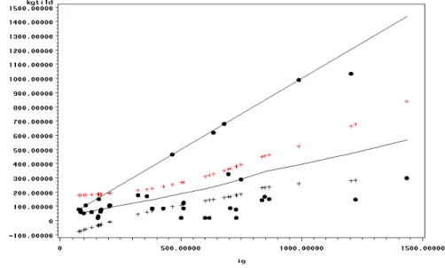
In order to assess the quality of our methodology, we propose to estimate the e¢ ciency function of public investments in road and highways for the United States over the period 1951-1992. We use the series of public investments (Federal, State and Local) in road and highways, valued at historical costs expressed in millions of US dollars (source BEA). For the corresponding physical measures, we consider the total road kilometers (Canning, 1998). Figure 1 displays the estimated e¢ ciency function and the corresponding 95% con…dence interval. We can observe that the estimated function is relatively close to the straight line of 45 slope. For a low level of investments, the estimated e¢ ciency function is statistically not di¤erent from the identity function. Consequently, for the United States, our approach does not show an important discrepancy between investments and the (net) variation of capital stocks. So, the PIM provides a good proxy of the public capital stocks e¤ectively available.
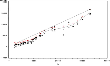
When the same methodology is applied for the case of our two reference de-veloping countries, the results are very di¤erent. Figure 2 displays the estimated e¢ ciency functions for electricity, road and telecoms sectors in Colombia over the period 1980-1994. It appears that the sector where public investments are the more e¢ cient is the telecommunication sector. However, these comparative results must be very carefully used. Given data availability, our sectorial samples are very reduced. It implies that the estimates of the sectorial e¢ ciency functions are relatively imprecise. So, in order to obtain more precise estimates, we pro-pose an estimate of the global e¢ ciency function based on the three sectors. More precisely, we report all the couples Kej;t+1; Ijt obtained for the sectors j = 1; 2
and 3 with eKj;t+1, the net variation in capital stock. Given these observations,
we estimate the global e¢ ciency function f (:) ; assumed to be homogeneous over
3The principle of this regression is that a local polynomial is estimated for every reference
point, using the points situated in the neighborhood of this reference point. The dimension of these neighborhoods is determined by a smoothing parameter which is de…ned by the rapport between the number of points included in the neighborhood and the total number of observa-tions. The smoothing parameter was chosen according to a modi…ed AIC criterion.
the three sectors, by a LOESS regression. e
Kj;t+1 = f (Ijt) j = 1; 2; 3 (13)
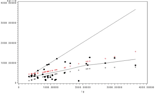
Figure 3 displays the estimated e¢ ciency function for Colombia and Figure 4 displays the same function for Mexico. Both estimated functions are strikingly similar. They show that the ”productive” component of public investments is largely overvalued when the PIM is used. Two results are particularly interesting here. Firstly, the estimated function is near a straight line. This conclusion is ro-bust to the choice of another information criterion as the general cross validation (GCV) function. It implies that the estimated function can be approximated by a simple linear functional form f (It) = Itwhere , with 0 < < 1;denotes an
e¢ ciency parameter according to the expression proposed by Pritchett (1996). In other words, the relative e¢ ciency, de…ned as the ratio of the ”productive”invest-ments to the total amount of invest”productive”invest-ments, is constant. Secondly, the coe¢ cient of the linear regression of eKj;t+1 to Ijt is equal to 0.38 in the case of Colombia
and 0.40 in the case of Mexico. According to this evaluation, one peso of public investments creates around 0.40 pesos of public capital in our reference sectors. So, our conclusions based on these non parametric estimates are similar to that of Pritchett (1996).
4
Conclusion
It is recognized that in a typical developing country, an important part of public investments may be ine¢ cient in creating capital. Consequently, the perpetual inventory method, based on monetary investment ‡ows, may overvalue the public stocks. So, we propose an original non parametric approach to evaluate the e¢ ciency function that links variations (net of depreciation) of stocks to public investments. We consider four sectors (electricity, telecommunications, roads and railways) of two Latin American countries (Mexico and Colombia). We show that there is a large discrepancy between the amount of investments and the value of increases in stocks. Moreover, the estimated e¢ ciency function is almost linear: the ratio of "productive" investments to the total investments is constant and equal to 0.38 in the case of Columbia and 0.40 in the case of Mexico.
A
References
Aschauer, D.A. (1989) ”Is Public Expenditure Productive?”Journal of Monetary Economics 23, 177-200.
Berndt E.R. and Hansson B. (1992) ”Measuring the Contribution of Public In-frastructure Capital in Sweden”Scandinavian Journal of Economics 94, 151-168. Bureau of Economic Analysis (2003) ”Fixed Assets and Consumer Durable Goods in the United Sates, 1925-1997”, Washington, U.S. Department of Commerce. Calderon, C., Easterly, W. and Serven, L. (2004) ”Latin America’s Infrastructure in the Era of Macroeconomic Crises”in The Limits of Stabilization by W. Easterly and L. Serven, Eds., The World Bank.
Canning D. (1998) ”A Database of World Infrastructure Stocks, 1950-1995”The World Bank Economic Review 12, 529-547.
Canning D. (1999) ”Infrastructure’s Contribution to Aggregate Output” World Bank Policy Research Working Paper, 2246, Washington D.C.
Cleveland, W. and Devlin S. (1988) ”Locally Weighted Regression: An Approach to Regression Analysis by Local Fitting” Journal of American Statistical Associ-ation 83, 596-610.
Easterly W. and Serven L. (2004) The Limits of Stabilization, The World Bank. Ford R. and Poret P. (1991) ”Infrastructure and Private-Sector Productivity” OECD Economic Studies 17, 63-89.
Gramlich E.M. (1994) ”Infrastructure Investment: a Review Essay” Journal of Economic Literature 32, 1176-1196.
Kamps C. (2004) The Dynamic Macroeconomic E¤ects of Public Capital: Theory and Evidence for OECD Countries, Springer.
Pritchett, L. (1996) ”Mind your P’s and Q’s. The cost of Public Investment is Not the Value of Public Capital” Policy Research Working Paper 1660, The World Bank.
Sturm J.E. (1998) Public Capital Expenditure in OECD Countries: the Causes and Impact of the Decline in Public Capital Spending, Edward Elgar.
Sturm J.E. and De Haan J. (1995) ”Is Public Expenditure Really Productive?” Economic Modelling 12, 60-72.
Table 1. Annual Depreciation Rates by Categories4
Categories Equipment Structures Depreciation Rate Road — 0.0202 0.0202 Railways 0.0589 0.0275 0.0328 Electricity 0.050 0.0211 0.0260 Gas — 0.0237 0.0237 Water — 0.0152 0.0152 Telecoms 0.1375 0.0237 0.0429
Note: For each asset, the depreciation rate is de…ned as a weighted average of the corresponding rates used for equipments and structures. The depreciation rates for equipment and structures are taken from Bureau of Eco-nomic Analysis (2003), table C, page M-31.
Figure 1 Non-Parametric Estimated E¢ ciency Function of Public Investments in Streets and Highways. United States, 1951-1992 (US$ million, Historical Cost)
Figure 2. Non-Parametric Estimated E¢ ciency Functions of Sectorial Public Investments. Colombia, 1980-1994 (US$ million, current prices)
Electricity Telecoms
Roads
Figure 3. Non-Parametric Estimated E¢ ciency Function of Total Public Investments. Colombia, 1980-1994 (US$ million, current prices)
Figure 4. Non-Parametric Estimated E¢ ciency Function of Total Public Investments. Mexico, 1980-1994 (US$ million, current prices)