Département de géomatique appliquée Faculté des lettres et sciences humaines
Université de Sherbrooke
ANALYSE DES CYCLES GEL/DÉGEL DES RÉGIONS NORDIQUES PAR TÉLÉDÉTECTION MICRO-ONDES PASSIVES EN BANDE L
Michaël Prince
Mémoire présenté pour l’obtention du grade de Maître ès sciences (M. Sc.), cheminement recherche en télédétection
Août 2018 ©Michaël Prince, 2018
ii
Identification du jury
Directeur de recherche :
Dr. Alain Royer, Professeur titulaire, Département de géomatique appliquée, Faculté des lettres et sciences humaines, Université de Sherbrooke
Co-directeur de recherche :
Dr. Alexandre Roy, Professeur, Département des Sciences de l’Environnement, Université du Québec à Trois-Rivières
Co-directeur de recherche :
Dr. Alexandre Langlois, Professeur agrégé, Département de géomatique appliquée, Faculté des lettres et sciences humaines, Université de Sherbrooke
Membres du jury :
Dr. Yannick Huot, Professeur agrégé, Département de géomatique appliquée, Faculté des lettres et sciences humaines, Université de Sherbrooke
iii
Résumé du projet
Le réchauffement climatique dans les régions nordiques, fort important depuis le milieu du siècle dernier, a de multiples impacts sur la dynamique des écosystèmes, notamment sur les cycles gel/dégel de surface qui influencent les flux de carbone, l'activité biogéochimique des sols, l'hydrologie et le pergélisol aux hautes latitudes. La télédétection satellitaire du gel/dégel par micro-ondes passives est un outil très prometteur permettant un suivi continu et global, mais comporte des difficultés souvent reliées à l’effet d’hétérogénéité spatiale intra-pixel relié aux résolutions grossières des capteurs micro-ondes passives à basse fréquence.
L’objectif principal du projet est d’évaluer l’utilisation de la télédétection micro-onde passive en bande L (1.4 GHz) pour le suivi de l’état de gel/dégel de la surface en forêt boréale. Un premier objectif spécifique est d’évaluer un nouveau produit des cycles de gel/dégel de surface estimée à partir des radiomètres bande L satellitaires Aquarius. Cette base de données de 3.5 années a été mise en ligne au National Snow and Ice Data Center (NSIDC). Le deuxième objectif spécifique est d’analyser l’effet de la variabilité spatiale intrapixel de l’état de gel du sol et de son impact sur les températures de brillance (TB) mesurées par le radiomètre de la mission Soil Moisture Active
Passive (SMAP) en période de transition afin de quantifier la fraction de sol gelé.
Les résultats pour le premier objectif montrent que la nouvelle base de données possède une bonne capacité à estimer l’état de gel/dégel de la surface sur l’ensemble de l’Hémisphère Nord (> 50°N). Cette recherche offre également une rare intercomparaison entre produits de gel/dégel satellitaires en comparant le produit Aquarius au Freeze/Thaw-Earth System Data Record (FT-ESDR) développé avec les données à plus hautes fréquences du capteur SSM/I. Pour le deuxième objectif, des capteurs de température distribués le long de transects de plusieurs kilomètres sur deux différents sites de taïga montrent que la variabilité spatiale du gel à l’automne peut être de 7.5 à 9.5 semaines. Il est également démontré que les mesures de SMAP sont sensibles à cette variabilité et un algorithme développé permet d’estimer le pourcentage intrapixel de sol gelé avec des coefficients de détermination (R2) entre 0.63 et 0.88 lorsque comparé aux mesures in situ. Ces résultats offrent de nouveaux outils pour mieux comprendre et quantifier les cycles de gel/dégel de l’environnement boréal et leurs impacts sur les processus biogéophysiques, hydrologiques et sur le pergélisol.
iv
Project Abstract
Climate change in nordic regions, which has been of growing significance over the past century has multiple impacts on the dynamic of ecosystems, notably on the surface freeze/thaw cycles, which influences carbon flux, soil biogeochemical activity, hydrology and permafrost at high latitudes. Satellite remote sensing of freeze/thaw with passive microwaves is a promising tool to offer continuous and global monitoring, but can also entail some difficulties due to intra-pixel spatial variability effects coming from the low resolution of low-frequency passive microwave sensors.
The primary objective of the project is to evaluate the use of passive microwave remote sensing in L-band (1.4 GHz) for monitoring of the surface freeze/thaw in the boreal forest. A first specific objective is to evaluate a new surface freeze/thaw product estimated by the Aquarius satellite L-band radiometers. This 3.5 year-old database has been put online at the National Snow and Ice Data Center (NSIDC) website. The second specific objective is to analyse the effect of intra-pixel spatial variability of freeze/thaw and its impact on brightness temperatures (TB) measured by the Soil Moisture Active Passive (SMAP) radiometer during transition periods in order to quantify the frozen soil fraction.
Results for the first objective show that the new database possesses a good capacity to estimate the surface freeze/thaw state for the entirety of the Northern Hemisphere (>50°N). This research also offers a rare intercomparison between freeze/thaw satellite products by comparing the Aquarius product to the Freeze/Thaw-Earth System Data Record (FT-ESDR) product developed with higher frequencies data of the SSM/I sensor. For the second objective, temperature sensors distributed along transects of several kilometers on two different taiga sites show that the spatial variability of autumn soil freeze onset can be between 7.5 and 9.5 weeks. It demonstrates that SMAP measurements are sensitive to this variability and a developed algorithm offers estimations of the intrapixel soil frozen fraction with coefficients of determination (R2) between 0.63 and 0.88 when compared to in situ measurements.
These results offer new tools for a better understanding and quantification of freeze/thaw cycles in boreal environments and their impacts on biogeochemical and hydrologic processes and on permafrost.
v Table des matières
Résumé du projet ... iii
Project Abstract ... iv
Liste des figures ... vi
Liste des tableaux ... viii
Liste des abréviations ... ix
Remerciements ... xi Avant-propos ... xii 1. Introduction ... 1 1.1 Contexte ... 1 1.2 Problématique ... 2 1.2 Objectifs ... 6 1.3 Hypothèses ... 7
2. Produit gel/dégel de surface en Bande L sur l’hémisphère nord conçu à partir des radiomètres satellitaires d’Aquarius ... 8
2.1 Présentation de l’article ... 8
2.2 Article 1 ... 10
3. Effets de la variabilité spatiale intra-pixel du gel/dégel de surface sur les mesures bande L du radiomètre satellitaire SMAP en forêt boréal ... 41
3.1 Présentation de l’article ... 41
3.2 Article 2 ... 42
4. Conclusion générale ... 65
vi
Liste des figures
Figure 1 : Permittivité électrique de l’eau (T= 273 K) et de la glace (T=273 K) en fonction de la
fréquence. ε’ est la partie réelle et ε’’ est la partie imaginaire. ε’’est nulle pour la glace aux fréquences de 1 à 100 GHz. ... 2
Figure 2: Série temporelle (2011-2013) du NPR avec estimation de l’état de gel/dégel (FT)
dérivé de SMOS et d’Aquarius en zone de toundra (en haut) et en zone de forêt boréale (en bas) (inspiré de Roy et al., 2015). ... 4
Figure A1-1: Land cover classes: tundra (blue), forest (green), open land (yellow) and water/ice
mask (white). Red dots show weather station locations ... 16
Figure A1-2: (a) Map of the percentage agreement between FT-AP and FT-ESDR classification
for the whole period studied and (b) derived frequency distribution of the mean percentage agreement over the whole study area (Lat. > 50° N). ... 18
Figure A1-3: Time series of percentage of frozen grid cells for FT-AP and FT-ESDR for the
three land covers (tundra, forest and open lands). ... 19
Figure A1-4: Freeze onset maps, where colors indicate the week of year, for a) 2011, b) 2012, c)
2013 and d) 2014 with FT-AP (top), FT-ESDR (middle) and difference between the products (Diff. = FT-AP minus FT-ESDR; bottom) ... 22
Figure A1-5: Thaw onset maps, where colors indicate the week of year, for a) 2012, b) 2013 and
c) 2013 with AP (top), ESDR (middle) and difference between the products (Diff. = FT-AP minus FT-ESDR; bottom) ... 25
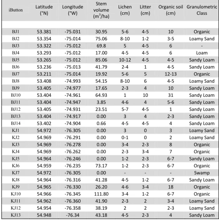
Figure A2-1: Baie-James – Le Moyne (BJ) site (Left) and Lac Chisapaw – Kuujjuarapik (KJ)
site (Right) showing iButton locations (red dots). The yellow rectangles delineate SMAP pixels. The intra-pixel water percentage from the SMAP L1C file is given in the middle of each pixel. Background: Landsat images from Google Earth. ... 45
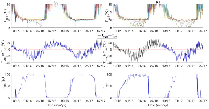
Figure A2-2: AM and PM (SMAP descending and ascending overpasses) soil temperature values
horizontal lines, respectively (top), vegetation and air temperatures, with 0°C represented by a red line (middle), and percentage of frozen soil from Ffro (bottom). BJ at left and KJ at right. ... 53
Figure A2-3: Time series of TBsim and TBSMAP AM and PM values (top), and NPRsim and
NPRSMAP (bottom). RMSE values with snow mask applied for each freeze period are given below the curves. BJ at left and KJ at right. ... 54
Figure A2-4 : Time series for 2015-2016 (top) and 2016-2017 (bottom) of the percentage frozen
soil estimated by SMAP (%frox) using the H, V and NPR observations compared to the percentage frozen soil observed by the iButtons (Ffro). BJ at left and KJ at right. The table in the lower right shows the regression line slope (m) and intercept (b) and R2 of the scatter graphs between Ffro and %frox calculated by combining the two years for each site. ... 56
viii
Liste des tableaux
Table A1-1: Thresholds (τ) applied in Eq. 3 for the whole circumpolar area, derived from the
Roy et al. (2015)………..………...12
Table A1-2: Latitude, longitude and land cover of each weather station ... 17
Table A1-3: Mean (μ), standard deviation (σ) and mean difference (Δμ) between products of freeze onset date (week of the year) for each land cover ... 23
Table A1-4: Means (μ), standard deviation (σ) and means difference between products of thaw onset date (week of the year) for each land cover ... 26
Table A1-5: Agreement (%) of weekly FT detections between FT-AP and FT-ESDR and between satellite products and in situ data (TAVGweek) for each site over the entire period. The sites are defined in Table 1. ... 27
Table A1-6: Product name, citation and URL for each dataset used in this study ... 34
Table A2-1: Coordinates, Stem Volume and Soil Characteristics for each iButton.. ... 46
Table A2-2: Percentage of each non-zero class from the LCCBU ... 47
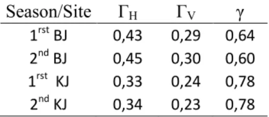
Table A2-3: ΓH, ΓV and γ values used to compute thawed TB (TBtha; Eq.1) for both the first and the second freezing season for BJ and KJ………..49
Table A2-4: ΓH, ΓV and γ values used to compute frozen TB (TBfro; Eq.1) for both the first and the second freezing season for BJ and KJ. The values for each site are the same for both seasons………49
ix
Liste des abréviations
%fro Frozen soil percentage in a pixel
FFrel Frost factor index
Ffro Fraction of frozen soil
FT Freeze/thaw
FT-ESDR Freeze/Thaw-Earth System Data Record
H et V Polarisation horizontale et verticale
IGBP International Geosphere-Biosphere Program
LCCBU Land Cover Classifications Derived from Boston University MODIS / Terra
Land Cover Data
MEaSUREs Making Earth System Data Records for Use in Research Environnements
NASA National Aeronautics and Space Administration
NASA/SAC-D Aquarius de la Satellite de Aplicaciones Cientificas
NDVI Normalized Difference Vegetation Index
NPR Rapport de polarisations normalisé (Normalized Polarization Ratio)
NSIDC National Snow and Ice Data Center
p Polarisation
RMSE Root mean square error
Rugg_Mean Resampled ruggedness
SAT Surface air temperature
SMAP Soil Moisture Active Passive
SMM/I Special Sensor Microwave Imager
SMMR Scanning Multi-channel Microwave Radiometer
SMOS Soil Moisture Ocean Salinity
SSMIS SSM/I Sounder
T1 and T2 Temperature thresholds for freeze/thaw classification (article 2)
TAVGday Average SAT for each day
TAVGweek Weekly resampled TAVGday
TB Température de brillance
WMO World Meteorological Organization
γ Vegetation transmissivity
Γp Soil reflectivity
Δεeau/glace Contraste des permittivités électriques entre l’eau et la glace
ε Permittivité électrique
τ Thresholds for freeze/thaw classification (article 1)
Remerciements
Je veux tout d’abord remercier mon directeur Alain Royer et mon codirecteur Alexandre Langlois. Leurs efforts constants permettent à un grand nombre d’étudiants de vivre des expériences d’une grande richesse. Je me sens très privilégié d’avoir été membre de leur magnifique équipe.
Je tiens à honorer spécialement mon second codirecteur, Alexandre Roy, avec qui j’ai eu la chance de m’entretenir presque quotidiennement. Faire de la recherche scientifique en sa compagnie, avec rigueur et passion, mais aussi avec humour et bonne humeur, a été un équilibre parfait qui m’a soutenu pendant ces deux dernières années. La qualité retrouvée dans ce mémoire lui est en grande partie due. Je lui souhaite succès et plaisir dans sa toute nouvelle carrière en tant que professeur à l’Université du Québec à Trois-Rivières.
Je veux également remercier les professeurs qui m'ont enseigné, soit Richard Fournier, Norman T. O’Neill et Kalifa Goïta. Leur savoir et leur passion ont influencé ce projet de recherche. Grâce à eux, je peux embarquer dans le marché du travail comme géomaticien (télédect.) avec plusieurs cordes à mon arc. Un gros merci également à tous mes collègues du département qui ont rendu ces deux années riches et agréables.
Cette maîtrise a été possible grâce à la contribution financière de l’Agence Spatiale Canadienne (ASC), du Conseil de Recherches en Sciences Naturelles et en Génie du Canada (CRSNG), la Fondation Canadienne pour l'Innovation (CFI), le Centre d’étude Nordique (CEN), le Programme de Formation Scientifique dans le Nord (NSTP) et le Fond de Recherche Nature et Technologiques (FRQNT). Il faut souligner que la base de données du gel/dégel d’Aquarius a été publiée grâce au support financier de la National Aeronautics and Space Agency (NASA) et avec le grand soutien de Ludovic Brucker.
Finalement, je dédie cette maîtrise à ma famille, soit ma conjointe Alison Brunette pour son infini support, mes filles Joëlle et Amy pour leur source d’amour et de joie, mes parents Pierre Prince et Johanne Blouin pour le support de toute une vie.
xii
Avant-propos
Ce mémoire est un mémoire par article. Les deux sous-objectifs sont respectivement traités dans les chapitres 2 et 3 dans deux articles. Le premier a été accepté pour publication dans Earth System Science and Data et le second, soumis à Remote Sensing of Environnement, est actuellement en révision.
Après une introduction présentant le contexte et les objectifs de recherche, ce mémoire est structuré autour de ces deux articles, contenant chacun la description des méthodologies utilisées, des résultats et des discussions. Une conclusion générale complète le document, ainsi que la liste des références bibliographiques non citées dans les articles.
1
1. Introduction 1.1 Contexte
La forêt boréale est le deuxième plus grand biome du globe comportant 33 % des régions forestières mondiales (FAO, 2001) et elle couvre 5.5 millions de km2 au Canada, soit plus de la moitié du territoire canadien. Le réchauffement climatique dans cette zone boréale, important depuis le milieu du siècle dernier (Gauthier et al., 2015; Ruckstuhl et al., 2008), a de multiples impacts sur la dynamique de cet écosystème, en particulier sur les cycles de gel/dégel de surface qui influencent la saison de croissance de la végétation (Kim et al., 2014), l'activité biogéochimique des sols (Panner Selvam et al., 2016), l'hydrologie (Beer et al., 2007), le pergélisol (Schuur et al., 2015) et les flux de carbone (Kim et al, 2012 ; Richardson et al., 2010; Barr et al., 2009). Notamment, la forêt peut passer de source de CO2 à un puits de CO2 les années
où la durée de gel est significativement réduite (Parazoo et al., 2018), car une longue saison de dégel peut engendrer une augmentation de la capacité de la végétation à capter le CO2, alors
qu’une saison plus courte va diminuer la saison de croissance et donc la captation de CO2 par la
végétation (Goulden et al., 1998). De plus, le couvert nival en zone boréale, directement lié aux conditions climatiques (précipitations et température), peut aussi jouer un rôle majeur dans cette dynamique par son effet isolant du sol (Gouttevin et al., 2012). Ainsi, mieux comprendre et suivre la variation des cycles de gel/dégel en lien avec le réchauffement climatique est un élément clé pour le suivi de la forêt boréale et sa réponse face à ces changements.
La capacité à observer globalement et quotidiennement l’état de gel/dégel du sol est limitée par la rareté des stations météorologiques, surtout dans les régions nordiques (Nalder and Wein, 1998). Même si les mesures in situ peuvent être interpolées en considérant la topographie et les caractéristiques des microclimats, ces méthodes ne pourraient fournir des informations suffisantes à l’échelle globale (New et al., 2000).
Les capteurs satellitaires dans les micro-ondes passives, qui dépendent de la radiation émise naturellement par la surface de la Terre, se sont avérés efficaces à détecter le gel/dégel de la surface et possèdent l’avantage d’enregistrer quotidiennement les températures de brillance (TB) à l’échelle planétaire, avec des mesures possibles autant le jour que la nuit ainsi, avec certaines
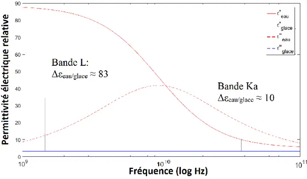
fréquences quasi insensibles aux conditions atmosphériques (Rautiainen et al., 2016; Roy et al., 2015; Kim et al., 2011). La raison est que dans les fréquences micro-ondes (entre 1 GHz et 50 GHz), la permittivité électrique (ε), qui influence l’émissivité du rayonnement électromagnétique (Demontoux et al., 2008), possède un fort contraste entre l’état gelé et dégelé de l’eau (Δεeau/glace; Artemov and Volkov, 2014; Figure 1). La résultante est que la TB subira une
augmentation marquée lors de la transition de phase de l’eau vers la glace et une diminution semblable pour le passage inverse.
Figure 1 : Permittivité électrique de l’eau (T= 273 K) et de la glace (T=273 K) en fonction de la fréquence. ε’ est la partie réelle et ε’’ est la partie imaginaire. ε’’est nulle pour la glace aux fréquences de 1 à 100 GHz.
1.2 Problématique
Il existe le produit Freeze/Thaw Earth System Data Record (FT-ESDR), un produit satellitaire de gel/dégel faisant partie du projet Making Earth System Data Records for Use in Research
Environnements (MEaSUREs) de la National Aeronautics and Space Administration (NASA). Le
produit offre des données du gel/dégel sur l’ensemble du globe pour une période continue s’étendant de 1979 jusqu’à 2016 (Kim et al., 2011; 2017). Il a été développé grâce à la série de capteurs Scanning Multi-channel Microwave Radiometer (SMMR), Special Sensor Microwave
dans une résolution spatiale de 25 km quatre états : gelé toute la journée, dégelé toute la journée, en transition (gelé le matin et dégelé l’après-midi), en transition inverse (dégelé le matin et gelé l’après-midi). Toutefois, les références in situ qui ont permis d’évaluer le produit se limitent strictement à la température de l’air (Kim et al., 2017). Quoiqu’il s’agisse d’une bonne indication du processus physique de l’état de l’environnement (Roy et al., 2015), étant donné l’interaction entre l’atmosphère et les surfaces, l’état du sol demeure incertain. De plus, l’algorithme du FT-ESDR se base uniquement sur la TB à 37 GHz en polarisation verticale, correspondant à une longueur d’onde d’environ 0,8 cm. La radiation à ces plus courtes longueurs d’onde peut fortement entrer en interaction avec l’ensemble des différents éléments se retrouvant dans un pixel (Ulaby et al., 1986). Il y a donc une grande incertitude à savoir exactement ce à quoi le signal gel/dégel est relié, et plus concrètement, à quel niveau le sol, la neige, la structure et la phénologie de la végétation contribuent au signal. De plus, à cette fréquence, le contraste des permittivités entre l’eau et la glace est plus faible.
Depuis les dernières années, une série de missions ont rendu possible l’observation satellitaire en bande L (1.4 GHz), telles que les missions Aquarius de la Satellite de Aplicaciones Cientificas (NASA/SAC-D; 2011-2015; Le Vine et al., 2010), Soil Moisture Ocean Salinity (SMOS) de la
European Space Agency (ESA; 2010-présent; Kerr et al., 2010) et dernièrement Soil Moisture Active Passive de la NASA (SMAP; 2015-présent; Entakhabi et al., 2010). Avec une longueur
d’onde d’environ 21 cm, la radiation captée dans cette bande devrait être moins sujette à interagir avec la végétation (Ulaby et al., 1986) et la neige sèche (Picard et al., 2013), puisque les branches et le feuillage des arbres et la taille des grains de neige sont beaucoup plus petits que la longueur d’onde. Il a été démontré que le rapport des TB en polarisation horizontale et verticale (H et V) diminue drastiquement à l’automne à cause de la chute de la constante diélectrique relié au gel du sol, demeure bas durant l’hiver et augmente significativement durant le printemps lorsque la constante diélectrique reprend des valeurs caractéristiques de sol dégelé (Derksen et al., 2017; Brucker et al., 2014; Rautiainen et al., 2012). D’autres études ont relié l’émission dans la bande L avec la profondeur de gel dans le sol (Rautiainen et al., 2014) et la température (Mironov et al., 2013). En somme, la télédétection en basse fréquence micro-ondes peut fournir de l’information différente et complémentaire sur le gel/dégel par rapport à celles fournies par des fréquences plus élevées, entre autres en étant plus sensible au contraste diélectrique relié aux gel/dégel du sol.
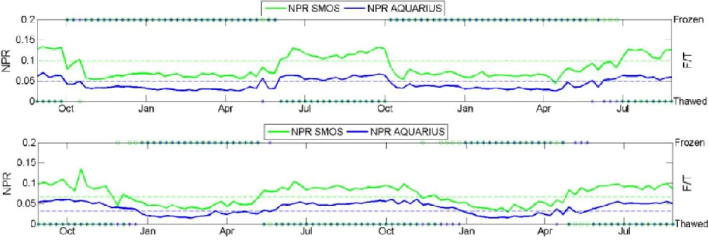
Dans ce sens, une étude approfondie des capteurs Aquarius et SMOS fut réalisée afin de vérifier la capacité à détecter le gel/dégel du sol en bande L par satellite (Roy et al., 2015). Cette recherche a entre autres estimé l’état de gel/dégel de surface en se basant sur le rapport de polarisations normalisé [NPR = (TBV -TBH)/ (TBV+TBH)] qui est un indice sensible à l’état de
gel/dégel (Rautiainen et al., 2014). Les résultats montrent que le NPR dans les régions de toundra change drastiquement lors des transitions intersaisonnières de gel/dégel de surface (Figure 2), avec des valeurs de NPR stables lors des périodes de gel hivernales et de dégel estivales. Par contre, dans les régions en forêt boréale, les transitions intersaisonnières sont moins distinctes, résultant à un taux de précision plus faible de la détection du gel/dégel lorsque les mesures satellitaires sont comparées aux valeurs in situ. Davantage de recherches doivent donc se réaliser pour déterminer l’effet du continuum sol/végétation sur la TB durant les périodes de gel/dégel en forêt boréale.
Figure 2: Série temporelle (2011-2013) du NPR avec estimation de l’état de gel/dégel (FT) dérivé de SMOS et d’Aquarius en zone de toundra (en haut) et en zone de forêt boréale (en bas) (inspiré de Roy et al., 2015).
De plus, de récentes études (Roy et al., 2017a; Lemmetyinen et al., 2016; Schwank et al., 2015, 2014) ont démontré que la neige « sèche » (sans présence d’eau liquide) a un certain impact sur la TB en bande L émise par le sol. La neige augmente la TB, allant dans le même sens que le signal engendré par un sol gelé. À l’opposé, la présence d’eau dans la neige absorbe la radiation et réduit la TB perçue par les radiomètres satellitaires, produisant un effet comparable à un dégel du sol (Roy et al., 2017a). Le couvert nival demeure donc une difficulté supplémentaire à surmonter
dans le but de comprendre le lien entre le signal en bande L et les conditions de gel/dégel des surfaces.
Actuellement, les produits satellitaires de gel/dégel classifient qualitativement l’état de surface, avec une approche à un seuil pour délimiter les deux classes (Kim et al., 2017; Derksen et al., 2017; Roy et al., 2015). Toutefois, les transitions de phase de l’environnement ne se réalisent pas abruptement et une coexistence des états se manifeste, particulièrement sur l’ensemble d’un territoire compris dans une empreinte de radiomètre satellitaire (entre 12 km et 40 km). Dans la méthode en conception du produit SMOS (Rautiainen et al., 2016), une classe « partiellement gelé » a été créée pour tenir compte de ce phénomène. Du côté de SMAP, une étude récente fait dans les prairies Canadiennes laisse entrevoir la possibilité que le radiomètre satellitaire soit sensible à la proportion de sols gelés à l’intérieur de ses pixels de 36 km de résolution (Rowlandon et al., 2018). En comparant le NPR dérivé des mesures de SMAP à des mesures in situ de gel/dégel sur plusieurs sites intrapixel durant quelques journées, le NPR a effectivement réagi proportionnellement à la quantité de surface gelée. De plus amples recherches doivent être menées pour valider la possibilité d’estimer une fraction de sol gelé dans un pixel à partir de la mesure satellitaire.
À ce jour, le seul produit offrant une estimation quotidienne sur le gel/dégel conçu en bande L sur l’ensemble du globe est celui de SMAP, alors que le nouveau produit Aquarius offre une information hebdomadaire. À noter qu’un produit SMOS (Rautiainen et al., 2016) est en développement, mais il n’est présentement pas disponible. De plus, à notre connaissance, aucun produit satellitaire en bande L n’a été comparé au FT-ESDR, qui est en bande Ka, pour observer des différences notables entre leurs estimations. Pourtant, il est connu que la bande L est la plus sensible à l’humidité du sol et qu'elle est moins affectée par la rugosité de la surface, la vapeur d’eau et la végétation (Kerr, 1996). À l’opposé, l’émission en bande Ka a une plus forte sensibilité à l’eau liquide des nuages, à la rugosité et à la végétation, mais elle est moins sensible à l’humidité du sol. Puisque la différence de permittivité électrique entre l’eau et la glace est plus grande en bande L (Δεeau/glace ≈ 83) qu’en bande Ka (Δεeau/glace ≈ 10) (Artemov and Volkov,
2014), la bande L devrait avoir un signal plus contrasté lors des transitions de phase dans le sol. Étant donné la relation entre la fréquence et le comportement physique du rayonnement
micro-onde, une comparaison entre produits de gel/dégel à différentes fréquences est nécessaire à la compréhension de l’information que procurent ces différents produits.
Finalement, il est crucial de mentionner que la principale difficulté de la télédétection satellitaire passive en micro-ondes est la résolution spatiale grossière des produits de TB, qui se situe
généralement entre 25 et 36 km (Derksen et al., 2017; Rautiainen et al., 2016; Brucker et al., 2014; Kim et al., 2011). L’effet de l’hétérogénéité de l’environnement comprise dans une telle superficie demeure une source d’incertitude et un défi à relever pour la communauté scientifique. Des campagnes de mesures sur le terrain et aéroportées ont mis en évidence la difficulté de relier la mesure de TB satellitaire à l’information sur l’ensemble du territoire sous le pixel (Roy et al., 2017b; Langlois et al., 2011; Derksen et al., 2005). La densité et le type de végétation, la présence d’étendues d’eau, la topographie, les caractéristiques du couvert nival (hauteur, densité, taille des grains), l’humidité, la rugosité et la composition du sol sont des facteurs influençant l’émission de micro-ondes. Ces paramètres peuvent varier au mètre près (Rutter et al., 2014), ne permettant pas de relier aisément une donnée in situ relativement ponctuelle à son pixel associé de la mesure satellitaire. À notre connaissance, il y a très peu d’études qui ont analysé l’impact de la variabilité spatiale des différentes composantes de l’environnement sur l’estimation de l’état de gel/dégel du sol en forêt boréale à l’échelle des pixels micro-onde passifs satellitaires.
1.2 Objectifs
L’objectif principal du projet est d’évaluer l’utilisation de la télédétection micro-onde passive en bande L (1.4 GHz) pour le suivi de l’état de gel/dégel de la surface en forêt boréale. Cette recherche est, entre autres, une contribution pour aider la caractérisation de la dynamique annuelle du cycle du carbone terrestre en lien avec la durée de gel du sol et la phénologie des écosystèmes boréaux. Deux objectifs spécifiques distincts, mais complémentaires permettent de répondre à l’objectif principal du projet.
Le premier objectif spécifique est d’évaluer un nouveau produit gel/dégel de surface estimé par les radiomètres satellitaires en bande L d'Aquarius que nous avons développé et mis disponible en ligne au National Snow and Ice Data Center (NSIDC) (Roy et al., 2018), ainsi que de le comparer au produit du Freeze/Thaw-Earth System Data Record (FT-ESDR) développé à partir des TB à 37 GHz.
Le deuxième objectif spécifique est d’analyser l’effet de la variabilité spatiale intrapixel de l’état de gel du sol à l’automne et de son impact sur la variation temporelle des signaux TB de SMAP en période de transition pour développer un nouvel algorithme permettant de quantifier la fraction de sol gelé.
Chacun de ces objectifs spécifiques fait l’objet d’un article scientifique. Le premier (section 2) est a été accepté pour publication et le second (section 3) est présentement en révision.
1.3 Hypothèses
L’hypothèse associée au premier objectif spécifique est :
Qu’il existe des différences entre les produits de gel/dégel d’Aquarius et du FT-ESDR puisqu’ils sont conçus à partir de fréquences micro-ondes différentes et que ces différences peuvent mener à des informations complémentaires sur l’état de la surface. Les hypothèses associées au deuxième objectif spécifique sont :
Que l’étude des températures de sol in situ distribuées spatialement va améliorer notre compréhension de l’effet de variabilité spatiale de l’état de gel/dégel du sol sur la TB mesurée en bande L en forêt boréale.
Que les TB mesurées par le radiomètre satellitaire de SMAP sont sensibles à la fraction de surface de sol gelé à l’intérieur d’un même pixel en forêt boréale permettant ainsi le développement d’un algorithme estimant la fraction de sol gelé.
2. Produit gel/dégel de surface en Bande L sur l’hémisphère nord conçu à partir des radiomètres satellitaires d’Aquarius
« Northern Hemisphere Surface Freeze/Thaw Product from Aquarius L-band Radiometers » Michael Prince1,2, Alexandre Roy3,2,1, Ludovic Brucker4,5, Alain Royer1,2, Youngwook Kim6, Tianjie Zhao7
1 Centre d’Applications et de Recherches en Télédétection (CARTEL), Université de Sherbrooke, Sherbrooke, QC
J1K 2R1, Canada
2 Centre d’Étude Nordique, Québec, Canada
3 Département des Sciences de l’Environnement, Université du Québec à Trois-Rivières, Trois-Rivières, QC,
Canada, G9A5H7
4 NASA Goddard Space Flight Center, Cryospheric Sciences Laboratory, Code 615, Greenbelt, MD 20771, USA 5 Universities Space Research Association, Goddard Earth Sciences Technology and Research Studies and
investigations, Columbia, MD 21044, USA
6 Numerical Terradynamic Simulation Group, College of Forestry & Conservation, The University of Montana,
Missoula, MT 59812, USA
7 State Key Laboratory of Remote Sensing Science, Institute of Remote Sensing and Digital Earth, Chinese Academy
of Sciences, Beijing, China
Article publié au Earth System Science Data (ESSD).
Référence:
Prince, M., Roy, A., Brucker, L., Royer, A., Kim, Y., and Zhao, T.: Northern Hemisphere surface freeze–thaw product from Aquarius L-band radiometers, Earth Syst. Sci. Data, 10, 2055-2067, https://doi.org/10.5194/essd-10-2055-2018, 2018.
2.1 Présentation de l’article
Cette étude évalue le nouveau produit de gel/dégel de surface conçu à partir des radiomètres d’Aquarius (FT-AP) selon l’algorithme développé par Roy (2015). Le produit est disponible sur le site de la NSIDC (https://nsidc.org/data/aq3_ft/versions/5). L’évaluation du produit s’est faite par une intercomparaison avec le produit FT-ESDR, sur la période de chevauchement des produits (2011-2014) sur l’ensemble de l’hémisphère nord au-dessus du parallèle 50°N. Cette analyse à grande échelle offre une intercomparaison entre produits issus de différentes bandes (L et Ka), permettant ainsi de mettre en évidence les ressemblances et les divergences qui pourraient provenir de la variation du comportement des micro-ondes selon les fréquences. De plus, cette analyse possède l’avantage de considérer la forêt boréale dans son entièreté, contenant également les régions de l’Eurasie, en plus de couvrir des régions de toundra et de milieux ouverts.
Pour cet article, ma contribution a consisté à l’analyse par intercomparaison des bases de données, à l’écriture et à la publication de l’article. De plus, j’ai contribué à la publication de la base de données FT-AP sur le site du NSIDC. Plus précisément, Alexandre Roy a initialement codé le programme pour faire rouler sur l’ensemble de l’hémisphère nord. J’ai validé la bonne qualité du produit et j’ai vérifé qu’il a été aplliqué convenablement. Puis, Ludovic Brucker a finalisé la base de données pour sa publication au NSIDC.
2.2 Article 1
Abstract. In the Northern Hemisphere, seasonal changes in surface freeze/thaw (FT) cycles are
an important component of surface energy, hydrological and eco-biogeochemical processes that must be accurately monitored. This paper presents the weekly polar-gridded Aquarius passive L-Band surface freeze/thaw product (FT-AP) distributed on the Equal-Area Scalable Earth Grid version 2.0, above the parallel 50° N, with a spatial resolution of 36 km x 36 km. The FT-AP classification algorithm is based on a seasonal threshold approach using the normalized polarization ratio, references for frozen and thawed conditions and optimized thresholds. To evaluate the uncertainties of the product, we compared it with another satellite FT product also derived from passive microwave observations but at higher frequency: the resampled 37 GHz FT Earth Science Data Record (FT-ESDR). The assessment was carried out during the overlapping period between 2011 and 2014. Results show that 77.1% of their common grid cells have an agreement better than 80%. Their differences vary with land cover type (tundra, forest and open land) and freezing and thawing periods. The best agreement is obtained during the thawing transition and over forest areas, with differences between product mean freeze or thaw onsets of under 0.4 weeks. Over tundra, AP tends to detect freeze onset 2–5 weeks earlier than FT-ESDR, likely due to FT sensitivity to the different frequencies used. Analysis with mean surface air temperature time series from six in situ meteorological stations shows that the main discrepancies between FT-AP and FT-ESDR are related to false frozen retrievals in summer for some regions with FT-AP. The Aquarius product is distributed by the U.S. National Snow and Ice Data Center (NSIDC) at https://nsidc.org/data/aq3_ft/versions/5 with the doi:10.5067/OV4R18NL3BQR.
1 Introduction
Seasonal freezing and thawing affect over half of the Northern Hemisphere. Landscape freeze/thaw (FT) state transitions show highly variable spatial and temporal patterns, with measurable influences to climate (IPCC, 2014; Peng et al., 2016; Poutou et al., 2004), hydrological (Gouttevin et al., 2012; Gray et al., 1985), ecological (Kumar et al., 2013; Black et al., 2000) and biogeochemical processes (Panneer Selvann et al., 2016; Xu et al., 2013; Schaefer et al., 2011). The surface FT state affects the latent heat exchange and the energy balance at the
interface between soil surface and the overlying medium. The vegetation growing season is sensitive to the annual non-frozen period (Kim et al., 2012), while vegetation net primary production and net ecosystem CO2 exchange with the atmosphere is impacted by FT timing
variability (Barr et al., 2009; Kurganova et al., 2007). Comprehensive in situ observational long-term datasets for soil state characteristics across terrestrial environments are still limited or inadequate, mostly for northern remote regions. Remote sensing in the thermal emission domain offers great potential for detecting changes in land-surface temperature, but is strongly limited by clouds, vegetation and snow cover (e.g. Langer et al., 2013). Spatially and temporally continuous information on soil freeze/thaw changes is lacking for the regions of both seasonal frozen ground and permafrost.
Passive microwave remote sensing has proven sensitive to the surface FT state due to large changes in surface dielectric properties between predominantly frozen and non-frozen conditions, and it offers global coverage. The remotely sensed FT detection capability at L-band (1.4 GHz) has been developed and validated in several studies (Zheng et al., 2017; Roy et al., 2017b; Rautiainen et al., 2012; Schwank et al., 2004). In the L-band, the shallow depth contributing to the radiation (around 5 cm for an unfrozen soil) and the strong permittivity difference between water and ice (Δεice/water) make it favourable for FT retrieval (Rautiainen et al., 2012; 2014). In
recent years, passive L-band FT algorithms were created for NASA’s Aquarius (Roy et al., 2015), ESA’s soil moisture and ocean salinity (SMOS) (Rautiainen et al., 2016), and NASA’s soil moisture active/passive (SMAP) (Derksen et al., 2017) missions. An FT Earth Science Data Record (FT-ESDR) was also produced using a higher microwave frequency at Ka-band (37 GHz) (Kim et al., 2017a). This product offers consistent and continuous global daily information on the FT state for several decades (1979-2016; Kim et al., 2017b). Observations were recorded by the scanning multi-channel microwave radiometer (SMMR), the special sensor microwave/imager (SSM/I), and the SSM/I Sounder (SSMIS).
This study presents the new Aquarius passive FT product for the Northern Hemisphere (Roy et al., 2018), distributed by the US National Snow and Ice Data Center (NSIDC) at https://nsidc.org/data/aq3_ft/versions/5. The product precision and uncertainties are addressed by comparing Aquarius FT retrievals with the FT-ESDR product for the overlapping period (2011 - 2014). The Aquarius passive FT product (referred to as FT-AP hereinafter) is based on the
Aquarius weekly Level-3 L-Band brightness temperature (TB) product (Brucker et al., 2015; NSIDC: http://nsidc.org/data/AQ3_TB/versions/5). The algorithm uses a relative frost factor (FFrel; see e.g. Rautiainen et al., 2014) based on normalized polarization ratio (NPR) temporal change detection (Roy et al., 2015). To our knowledge, few intercomparisons between L- and Ka-band FT products exist (Derksen et al., 2017), and none evaluated inter-annual variability differences. However, it is well established that different frequencies interact differently with ground components (vegetation, soil, snow), canopy, etc. For instance, observations at L-band are less sensitive than at Ka-band to snow, plant biomass and surface roughness (Ulaby et al., 1986). Being less prone to disturbances above the ground, the L-band emission should give better information on the ground state in forested and snow-covered areas. In addition, since Δεice/water is
larger at L-band (Δεice/water ≈ 83) than at Ka-band (Δεice/water ≈ 10) (Artemov and Volkov, 2014),
there should be a higher sensitivity to the ground phase transition at L-band. Hence, because differences between products can be attributed to the microwave frequency and the algorithm used, the FT-AP is also compared with surface air temperature (SAT) observations.
The main objective of this study is to present and evaluate the weekly FT-AP by comparing it to the FT-ESDR and to SAT observations across the Northern Hemisphere. First, we describe the new FT-AP product, designed by the algorithm developed by Roy et al. (2015), but applied across the Northern hemisphere. Then, we investigate the spatial and temporal FT variations from both FT-AP and FT-ESDR products over the Northern hemisphere. We then investigate the cause of the main differences between products from in situ information. The comparison aims to identify the similarities and differences between L-band and Ka-Band FT products for further improvements of FT monitoring across the Northern hemisphere.
2. Method
2.1 Aquarius passive FT product (FT-AP)
The Aquarius FT product was generated using the Aquarius weekly averaged polar gridded L-band TB product distributed on the EASE-Grid 2.0, above the parallel 50° N, with a spatial resolution of 36 km x 36 km (Brucker et al., 2014). This formatted TB was specially designed for the study of northern regions. For each Aquarius radiometers, the product averages TB values
calculated from every measurement made during a week, combining ascending and descending orbits. The FT classification algorithm is based on a seasonal threshold approach (STA) using frost factor index (FFrel) (Eq. 1), introduced by Rautiainen et al. (2014), where FFNPR is the frost
factor based on the normalized polarization ratio between TB at vertical and horizontal polarizations (TBV and TBH; Eq. 2). FFfr and FFth are reference frozen and thawed frost factors
obtained for each pixel and each radiometer by averaging, respectively, the five minimum FFNPR
found during winters (January and February) and five maximum FFNPR found during summers
(July and August) over the three available dataset period.
(1)
(2)
A threshold (τ) was determined by optimization to classify the surface as frozen or thawed if the FFrel is lower or higher than the threshold (Eq. 3).
If FFrel < τ → freeze
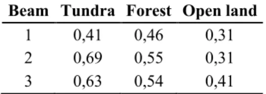
or if FFrel > τ → thaw (3) The thresholds optimized (Table 1) in Roy et al. (2015) over Northern America for three basic land covers (tundra, forest, open land) were applied over the Northern Hemisphere using the Land Cover Classifications derived from Boston University MODIS / Terra Land Cover Data (LCCBU) (see Sect. 2.4). The optimization method calculates the threshold that gives the best
accuracy when the product retrievals is compared to in situ air temperature stations. It was shown that optimized thresholds only slightly improved the accuracies by 1% to 4% compared to a fixed threshold of 0.5. For tundra site, a broad range of threshold values ([0.3-0.7]) caused an insignificant variation of accuracy.
Table 1: Thresholds (τ) applied in Eq. 3 for the whole circumpolar area, derived from the Roy et al. (2015)
Beam Tundra Forest Open land
1 0,41 0,46 0,31 2 0,69 0,55 0,31 3 0,63 0,54 0,41
Aquarius operated three non-scanning radiometers at different incidence angles (29.2°, 38.4° and 46.3°) and with different 3 dB footprint sizes (respectively 76 km x 94 km, 84 km x 120 km and 97 km x 156 km). Based on the LCCBU, the thresholds found in Roy et al., (2015) were used to
create FT maps for each radiometer. The three FT maps were then blended to create a fourth map, which offers more complete spatial coverage. For every grid cell, radiometer 2 (38.4°) was prioritized, then radiometer 1 (29.2°) was used, while radiometer 3 was only used if data from the other radiometers were not available for the given grid cell. This blended algorithm was chosen based on the performance given for each radiometer in Roy et al. (2015) (radiometer 2 gave the best results, while radiometer 3 gave the worst results). Due to the width of Aquarius’ swath and its revisit time, 16.5% of the terrestrial 36-km grid cells have less than 95% observations over the period and 16% were not measured at all. Thus, the intercomparison with the FT-ESDR product (Sect. 2.2) was only made when FT-AP data were available for a given date. The time span for this analysis runs from August 2011 with the first Aquarius observations to 31 December 2014 with the latest FT-ESDR data available at the time of our analysis.
2.2 FT-ESDR product
The first version of the FT-ESDR product (Kim et al., 2011) was based on an STA similar to the FFrel but applied exclusively to the TBV at 37 GHz instead of the NPR. In the new extended
product (Kim et al., 2017b; NSIDC: https://nsidc.org/data/nsidc-0477/versions/4), a modified seasonal threshold algorithm (MSTA) was used to determine thresholds for each grid cell to obtain better accuracy. It consists of a grid-cell-wise weighted empirical linear regression relationship between the 37 GHz TBV measurements and daily surface air temperature estimates
from the ERA-Interim global reanalysis.
The extended FT-ESDR product used in this study is derived from the SSM/I 37 GHz brightness temperatures (footprint of 38 km x 30 km) and resampled at a grid cell resolution of 25 km on the global Ease-Grid v1.0. The observations were recorded twice per day, which gives the possibility of attributing discrete frozen or thawed states for morning and afternoon. The final classification offers four discrete surface states: “frozen all day”, “thawed all day”, “frozen in AM and thawed in PM” (transitional) and “thawed in AM and frozen in PM” (inverse-transitional). In this study, the latter two classes were combined into a single transitional class. In order to compare the two
products, the FT-ESDR was first spatially resampled to the EASE-Grid 2.0 with the nearest neighbor method choosing the smallest distance between pixel centers. Then, FT-ESDR was temporally resampled at the same weekly calendar than the FT-AP. The temporal FT-ESDR sampling procedure was based on the rule that the most frequently occurring class over the seven days of a week is adopted as the value for the entire week. In cases where the frozen and thawed classes occurred with equal frequency during a single week (e.g. two days frozen, two days thawed and three days transitional), the transitional class was attributed. This latter class occurs mainly during the transition seasons of spring and fall. Thus, we assigned the transitional class to thawed class during spring and summer since it indicates the beginning of the thawing process and we assigned the transitional class to the frozen class during fall and winter since it indicates the beginning of the freezing process. This FT-ESDR resampling procedure ensured that the two products were at the same temporal and spatial resolutions with only the frozen and thawed categories, making comparison possible.
2.3 Land cover classification
The land cover information (Fig. 1) comes from the EASE-Grid 2.0 LCCBU (Brodzik and
Knowles, 2011; NSIDC: nsidc.org/data/nsidc-0610/versions/1), using the same grid as the FT-AP product. The seventeen land cover classes were grouped to obtain four classes: tundra, forest, open land (savanna, cropland and grassland) and water (see Roy et al., 2015). Each grid cell was assigned its single most prominent class of land cover which is used for the selection its thresholds (Table 1). All grid cells with more than 20% of water and ice indicated by the LCCBU
3 Figure 1: Land cover classes: tundra (blue), forest (green), open land (yellow) and water/ice mask (white). Red dots show weather station locations
2.4 Weather stations
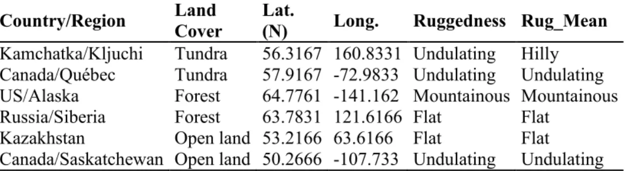
Six weather stations (Table 2) were selected for validation from the National Climatic Data Center (NCDC) Climate Data Online website (CDO, https://www.ncdc.noaa.gov/cdo-web/datasets). Two tundra, two forest and two open land sites were chosen for a comparison between the product classifications and the in situ SAT. All of the sites are more than 200 km from a coast, except the Kamchatka site; its distance of about 85 km from the sea may have an influence on the large L-band field of view. The average SAT for each day (TAVGday) were used
to create a time series for each site. For statistical purposes, the weekly resampling method used on the FT-ESDR product was also applied to the SAT daily values, using 0°C as the threshold between frozen and thawed states (TAVGweek) (see Roy and al., 2015).
Ruggedness values from a 30 arc-second resolution elevation map (Gruber 2012; University of Zurich: http://www.geo.uzh.ch/microsite/cryodata/pf_global/) were resampled to the EASE-Grid 2.0 with the drop in the bucket approach. In order to represent a ruggedness value at the Aquarius footprint scale, the mean value of a 3 x 3 grid cell window centered on each weather station pixel was calculated (Rug_Mean). To each value was attributed a class according to the Gruber (2012) classification.
1 Table 2: Latitude, longitude and land cover of each weather station (See also Fig.1)
Country/Region Land Cover Lat. (N) Long. Ruggedness Rug_Mean
Kamchatka/Kljuchi Tundra 56.3167 160.8331 Undulating Hilly Canada/Québec Tundra 57.9167 -72.9833 Undulating Undulating US/Alaska Forest 64.7761 -141.162 Mountainous Mountainous Russia/Siberia Forest 63.7831 121.6166 Flat Flat
Kazakhstan Open land 53.2166 63.6166 Flat Flat
Canada/Saskatchewan Open land 50.2666 -107.733 Undulating Undulating
3 Results
3.1 Spatial FT analysis
Figure 2a shows the percentage of concordant classifications between the two products for the 3.7 year overlapping period. Overall, the results show that there is good agreement between the two products. In general, forest areas have a better percentage of concordance than other land covers. However, some regions show important discrepancies, especially along coastal margins and in mountainous and open areas (such as in northern Europe, Kazakhstan (and surroundings) and the Canadian Prairies). Those lower percentages correspond to regions where lower accuracies to detect the FT were already noted in Roy et al. (2015) and Kim et al. (2017a) (see Sect. 4). Figure 2b shows that 77.1% of the common grid cells have more than 80% agreement. More specifically, 41.6% of the grid cells have more than 90% agreement over 3.7 years, with 10.0% of them having more than 95%. About 35.5% of the grid cells have an agreement between 80% and 90%; only 22.8% of the cells have an agreement lower than 80%.
(a)
(b)
4 Figure 2: (a) Map of the percentage agreement between FT-AP and FT-ESDR classification for the whole period studied and (b) derived frequency distribution of the mean percentage agreement over the whole study area (Lat. > 50° N).
3.2 Temporal analysis
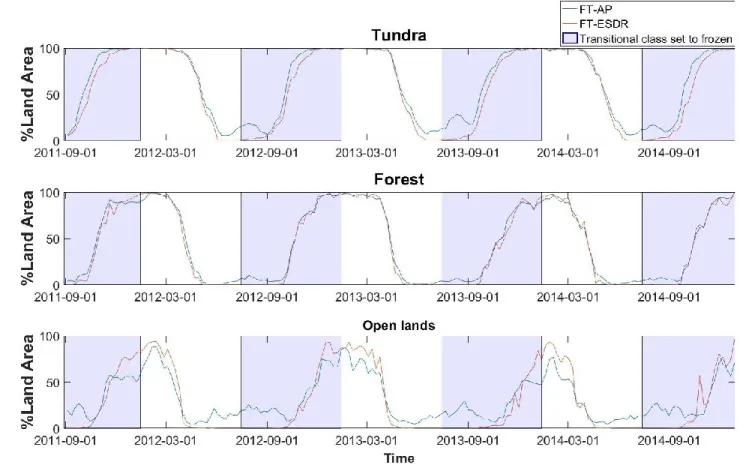
An analysis was made to identify similarities and differences between the two products used for retrieving surface FT state during the freezing (fall) and thawing (spring) periods. For each land cover type, Figure 3 shows the time series of the fraction of land frozen (for all land at latitudes greater than 50° N). To reduce the effect of obvious false frozen retrievals in summer (discussed below) on the analysis and to focus on the differences primarily related to the physics of the measurements (i.e., L-band vs. Ka-band), only grid cells with an agreement percentage between FT-AP and FT-ESDR higher than 80% (from Fig. 2a) were considered. Light blue zones indicate periods for which the FT-ESDR transitional class is set to the frozen class (see Sect. 2.2).
5 Figure 3: Time series of percentage of frozen grid cells for FT-AP and FT-ESDR for the three land covers (tundra, forest and open lands).
Figure 3 gives information on temporal differences between the products. The difference between FT-AP and FT-ESDR in terms of the percentage of frozen grid cells for a given day (Δ%frozen) is greatest during falls in tundra, at 10–27%. In forest, Δ%frozen is much lower than in tundra,
with differences of 0–12%. For these two land covers (tundra and forest), the agreement between the products varies by year. In fall, the horizontal shift between the curves indicates time delays (Δtime) for the two products to reach the same percentage of frozen grid cells. In tundra, Δtime ranges from 1–3 weeks. In forest, Δtime is always less than one week. This result demonstrates an excellent overall consistency between the products. However, FT-AP shows the percentage of frozen land increasing every summer to a peak that is not perceived with FT-ESDR. In tundra, those maximum values vary between 17% (2014) and 28% (2013) and are lower in forest at 7% (2013) and 10% (2012). Even if some of those detections represent the real state of the surface, the FT-AP peaks may be mainly caused by false frozen detections, which were noticed in the SMAP product (Derksen et al., 2017). False frozen detections are identified in our analysis using observations from the weather stations (Fig. 6, Sect. 3.3). In open land, FT-AP retrievals tend to vary frequently by showing noticeable unexpected frozen retrievals in summer and thawed retrievals in winter (blue lines in Fig. 3). FT-ESDR shows almost no frozen regions in summer, but unfrozen regions in winter, evidence that the open land regions are at the southern limits of the freeze regions. This in turn makes retrieval more difficult due to the higher temporal variability in FT events in winter.
To spatially represent the information provided by Δtime, maps in Fig. 4 indicate the week of the year of the freeze onset for each product (top and middle maps). The freeze onset is defined as the first week of the year when the state changed from thawed to frozen and stayed frozen for two more consecutive weeks. This variable can only be identified for grid cells that contain observations over several weeks in a row and have good agreement (>80%) according to Fig. 2a. Figure 4 also shows the difference in freeze onset between the two products (bottom maps), defined as FT-AP minus FT-ESDR. A negative value means that FT-AP detects the freeze onset earlier than FT-ESDR (represented by cold colors) and inversely for a positive value (represented by warm colors).
Comparing FT-AP and FT-ESDR maps shows a global tendency of FT-AP to reach the freeze onset 2–5 weeks earlier than FT-ESDR in the tundra regions (blue zones in Fig. 4). In 2013 and 2014 (Fig. 4c–d), this tendency is stronger, with more regions experiencing an earlier freeze onset by 3–5 weeks according to FT-AP. While these differences are less noticeable in the forest, some local discrepancies are observable with noticeable inter-annual variabilities.
6 Figure 4: Freeze onset maps, where colors indicate the week of year, for a) 2011, b) 2012, c) 2013 and d) 2014 with FT-AP (top), FT-ESDR (middle) and difference between the products (Diff. = FT-AP minus FT-ESDR; bottom)
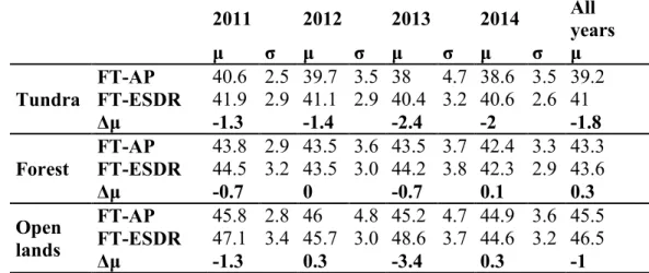
Table 3 gives freeze onset means (μ) and standard deviations (σ) in weeks of the year for each land cover and year. Over tundra, it shows the greatest freeze onset mean difference (Δμ = μFT-AP
minus μFT-ESDR) between the two products in 2013, with Δμ = 2.4 weeks, and the smallest
difference in 2011, with Δμ = 1.3 weeks. Over forest, the differences are much smaller; the greatest occurs in 2011, with Δμ = 0.7 weeks, and the smallest in 2012, with Δμ = 0.0 weeks. As noted for Fig. 4, FT-AP tends to detect freeze onset earlier than FT-ESDR. These freeze onset differences suggest that there is a divergence in the FT signal at L and Ka bands, and that there might be complementary information in the two signals (this is further addressed in the discussion).
2 Table 3: Mean (μ), standard deviation (σ) and mean difference (Δμ) between products of freeze onset date (week of the year) for each land cover
2011 2012 2013 2014 All years μ σ μ σ μ σ μ σ μ Tundra FT-AP 40.6 2.5 39.7 3.5 38 4.7 38.6 3.5 39.2 FT-ESDR 41.9 2.9 41.1 2.9 40.4 3.2 40.6 2.6 41 Δμ -1.3 -1.4 -2.4 -2 -1.8 Forest FT-AP 43.8 2.9 43.5 3.6 43.5 3.7 42.4 3.3 43.3 FT-ESDR 44.5 3.2 43.5 3.0 44.2 3.8 42.3 2.9 43.6 Δμ -0.7 0 -0.7 0.1 0.3 Open lands FT-AP 45.8 2.8 46 4.8 45.2 4.7 44.9 3.6 45.5 FT-ESDR 47.1 3.4 45.7 3.0 48.6 3.7 44.6 3.2 46.5 Δμ -1.3 0.3 -3.4 0.3 -1
For the thawing period, differences between the products according to Fig. 3 and Table 4 are small for all land covers, meaning that globally the two products respond similarly to landscape thaw. This result is consistent across land covers and for the three spring seasons available for this analysis with a stronger variability for open lands. The sensitivity of passive microwave frequencies to the water present in the snow at the beginning of the thaw explains the similarity between the products in spring (Roy et al., 2017a; Hallikainen et al., 1986). Thaw onset maps created from the difference of thaw onset between the products (bottom maps), defined as FT-AP minus FT-ESDR, illustrate the consistency between products, but highlight some local differences (Fig. 5).
7 Figure 5: Thaw onset maps, where colors indicate the week of year, for a) 2012, b) 2013 and c) 2013 with AP (top), FT-ESDR (middle) and difference between the products (Diff. = FT-AP minus FT-FT-ESDR; bottom)
3 Table 4: Means (μ), standard deviation (σ) and means difference between products of thaw onset date (week of the year) for each land cover
2011 2012 2013 All years μ σ μ σ μ σ μ Tundra FT-AP 19.1 3 19.1 3.2 18.8 3.6 19.0 FT-ESDR 18.7 2.3 18.7 2.4 18.8 2.5 18.7 Δμ 0.4 0.4 0 0.3 Forest FT-AP 14.7 2.3 15.4 2 13.7 3 14.6 FT-ESDR 14.3 2 15.3 1.5 14 2.4 14.5 Δμ 0.4 0.1 -0.3 0.1 Open lands FT-AP 11.9 2.4 13.3 3 11.2 3.5 12.1 FT-ESDR 12.1 1.9 14 1.7 11.6 2.9 12.6 Δμ -0.2 -0.7 -0.4 -0.4
3.3 Comparison with weather stations
In Sect. 3.1, it was shown that there were some regions where both products show significant discrepancies. In order to better assess the observed variabilities, we looked at six different sites (Fig. 1) to evaluate the temporal evolution of both FT products and compared them to SAT measurements. The objective was to identify any difficulties the products may have monitoring FT in particular conditions. SAT was chosen as in situ reference since Roy et al. 2015 showed that SAT was the best proxy to validate satellite FT products. Table 5 shows the percentages of agreement of weekly FT detection over the entire period between FT-AP, FT-ESDR and TAVGweek (Fig.6a-f). The mean agreement between the satellite products and in situ
measurement is 81.6% for FT-AP and 92.0% for FT-ESDR. Discontinuities in the series (Fig.6a-f) is caused by the absence of Aquarius observations in a given week.
4 Table 5: Agreement (%) of weekly FT detections between FT-AP and FT-ESDR and between satellite products and in situ data (TAVGweek) for each site over the entire period. The sites are defined in Table 2.
Country/Region Land Cover
FT-AP / FT-ESDR (%) FT-AP / TAVGweek (%) FT-ESDR / TAVGweek (%) Kamchatka/Kljuchi Tundra 68.7 67.9 94.3 Canada/Québec Tundra 83.8 90.8 89.7 US/Alaska Forest 87.7 88.9 94.3 Russia/Siberia Forest 97.1 97.7 97.1
Kazakhstan Open lands 66.3 70.9 92.0
Canada/Saskatchewan Open lands 76.2 73.3 84.6
Mean 80.0 81.6 92.0
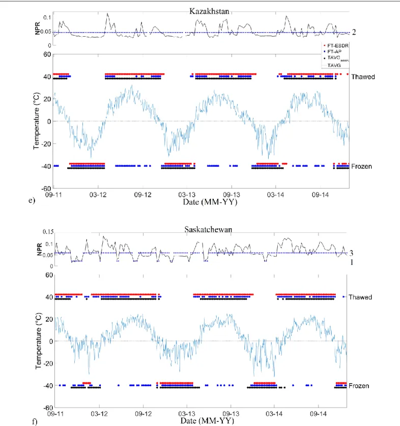
At the Kamchatka site (Fig. 6a, Table 5), FT-AP has a low agreement with TAVGweek at 67.9%.
The error occurs mostly in summers with obvious false frozen misclassifications, since SAT is over 0°C during that period. In contrast, there is a strong agreement of 94.3% between FT-ESDR and TAVGweek, with differences occurring in the transitional period with no specific pattern
between the years. The difficulty in the retrieval could be due to the fact that the Kamchatka site’s grid cell has a very low difference between the minimum and maximum NPR values (ΔNPR)
used to create FFfr and FFth, with ΔNPR = 0.015 and ΔNPR = 0.021 for radiometers 2 and 3,
respectively. This low difference may lead to a lower sensitivity to FT. Moreover, there is change of ruggedness classification (Table 2) from the one grid cell ruggedness (SSM/I footprint scale) to the Rug_M (Aquarius footprint scale) from undulating to mountainous. With a coastline at about 85 km, a major difference of spatial variability exists between SSM/I and Aquarius measurements over the Kamchatka site.
The Quebec site (Fig. 6b), also over tundra land cover, has better product agreements with TAVGweek than the Kamchatka site, with percentages around 90%. FT-AP has generally a better
agreement with TAVGweek during the fall freezing periods. There are only minor exceptions due
to a few false frozen retrievals in summer. These exceptions show a typical situation in which FT-AP detects the freeze onset earlier than FT-ESDR, as mentioned in Sect. 3.2. The relatively high ΔNPR (ΔNPR = 0.024 and 0.032 for radiometers 1 and 2, respectively) could be a factor
For forest sites (Fig. 6c–d), both products have good agreement with TAVGweek. The statistics for
the Siberia site highlight the highest agreement: 97.7% for FT-AP and 97.1% for FT-ESDR. Interestingly, the forest sites have ΔNPR values comparable to those of the tundra sites, with
ΔNPR = 0.022 and 0.029 for radiometers 2 and 3 respectively in Siberia, and a unique
ΔNPR = 0.010 for radiometer 1 in Alaska. The latter value is the lowest of all the sites in this
study. Since Alaska has relatively good FT-AP agreements (87.7% with TAVGweek and 88.9%
with FT-ESDR), clearly small differences between FFfr and FFth alone cannot explain the false
frozen retrieval problem at L-band.
At the open land sites, the low agreement (Fig. 6e–f) between FT-AP and TAVGweek (70.9% in
Kazakhstan and 73.3% in Saskatchewan) is mainly due to the false frozen retrieval in summer. During the transitional period, the FT-AP is in good agreement with TAVGweek, sometimes better
than ESDR, especially in the fall of 2012, 2013 and 2014 in Kazakhstan. Nevertheless, FT-ESDR agrees relatively well, with 92.0% in Kazakhstan and 84.6% in Saskatchewan. The winter of 2011 in Saskatchewan was particularly warm, and the products reacted differently to a succession of over 0°C events, which affected the overall agreement percentage. The ΔNPR of the
open land sites are 0.088 for radiometer 2 in Kazakhstan and 0.029 and 0.095 for radiometers 1 and 3 in Saskatchewan. Consequently, since these are the highest values of all sites, in this case, the false frozen retrievals cannot be explained by a small value of ΔNPR.
Figure 6. FT detection for each reference site (see Table 2), with FT-ESDR (red dots) and FT-AP (blue dots) against surface air temperature (black dots and blue line) in a) Kamchatka, b) Quebec, c) Alaska, d) Siberia, e) Kazakhstan and f) Saskatchewan.
NPR series (top) contain the combination of available Aquarius observations following the prioritization of radiometer 2, radiometer 1 and then radiometer 3 (sect. 2.1). NPR threshold values (blue dot) according to Eq.1 with the corresponding beam
Comparing both products to SAT at different sites shows that FT-AP tends to identify false frozen retrieval in summer periods. It is out of the scope of this paper to explain why these misclassifications occur, but some hypotheses will be given in Sect. 4.
4. Discussion
This study shows that overall FT-AP agrees well with weekly averaged SAT and with the Ka-Band FT-ESDR. Despite its being a weekly product, FT-AP has good sensitivity to the FT state of the landscape. Despite some regional discrepancies in forested landscape, very good agreements between FT-AP and FT-ESDR were found in this land cover, suggesting that the sensitivity of L- and Ka-bands to FT are more similar in forested landscape.
However, the study reveals that in certain regions, FT-AP seems to give false identifications of freezing surface in summer. These findings concord with other L-band FT analyses using SMAP and SMOS (Derksen et al., 2017; Rautiainen et al., 2016). Some regions like the coastlines, Kamchatka, Kazakhstan, Scandinavia, northern Europe, Alaska, the Canadian Rockies and the Canadian Prairies show agreement below 80% between FT-AP and FT-ESDR. An attempt was made to explain the false frozen retrievals occurring in the Kamchatka site and the two open land sites by looking at the ΔNPR values, but no direct relationship was observable. Relatively small
ΔNPR are found for Kamchatka, but they are similar to those of Siberia, which has agreement
higher than 95% with TAVGweek. The Alaska site has the smallest ΔNPR of all the sites but does
not possess the false frozen retrieval problem. To the contrary, the open land sites have the highest ΔNPR values and both have frozen retrievals during summer. Hence, ΔNPR can explain
some of the weak classifications, but not all of them.
The false freeze classification in open land regions could be related to the crop growth cycle. The growing vegetation leads to a stronger emission from the vegetation in both horizontal and vertical polarization (Gherboudj et al., 2012), causing a depolarization of the signal that decreases the NPR. This creates a similar effect to the FT signal and could lead to false freeze identifications in summer (Roy et al., 2015; Rautiainen et al., 2016). Another important factor that could influence the precision of L-band FT retrieval is the possibility of low soil moisture before freezing. Since the FT retrieval is based on Δεice/water, low soil moisture will lead to a low