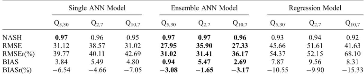
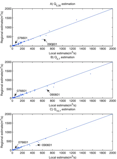
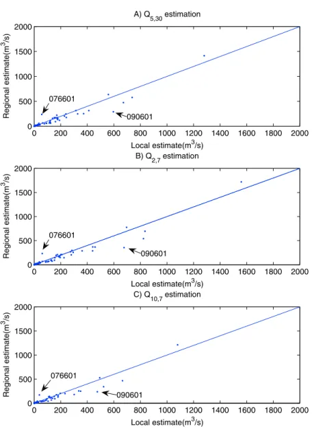
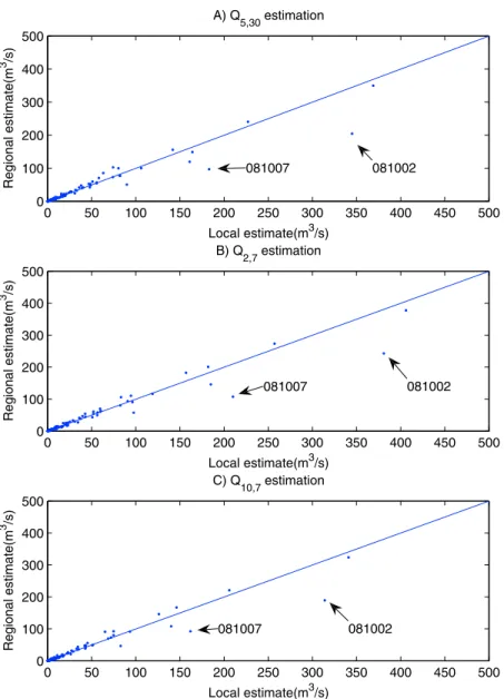
Regional low-flow frequency analysis using single and ensemble artificial neural networks.
Texte intégral
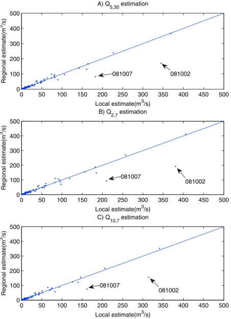
Figure


Documents relatifs
La consultation de suivi à 1 mois après une diversification du régime alimentaire associée à une supplémentation orale en vitamine C, B9 et D, montrait une amélioration franche
L’archive ouverte pluridisciplinaire HAL, est destinée au dépôt et à la diffusion de documents scientifiques de niveau recherche, publiés ou non, émanant des
26 * لﻘﻨ لﺎﺼﻴ ٕاو تﺎﻤوﻠﻌﻤﻝا : » لﺜﻤﻴ اذﻫ عرﻔﻝا ﺔﻴﻠﻤﻋ لﻘﻨ لﺎﺼﻴ ٕاو تﺎﻤوﻠﻌﻤﻝا ﻲﺘﻝا مﺘ ﺎﻬﻠﻴﻐﺸﺘ نﻴﺒ ﻊﻗاوﻤﻝا ةدﻋﺎﺒﺘﻤﻝا بﻴﺴاوﺤﻠﻝ أ و نﻴﺒ بﻴﺴاوﺤﻝا ادﺤوو ﻬﺘ
Simulation of experimental P profiles obtained after annealing in a wide temperature range gives satisfactory results, taking into account a quadratic de- pendence of the P
par voie Radiologique (GPR) - Fiche de synthèse de la RMM - Date de la RMM : Période analysée : Nombre d’évènements indésirables : Etablissements Participants Nombre de
Le style est l'homme même ، وC^ج رايب هفرع امك Pierre Guiraut هنأب " : ةباتكلا ي= ةقيرط " ) 10 (. اشيم امأ C^تافير ل Michael Riffaterre
Dans un environnement mouvant, et incertain, caractérisé par la mondialisation et forte concurrence, les entreprises se trouve confrontées à l’impératif d’être
Still, no discontinuity in connection to electricity is observed at all the other borders between Cote d’Ivoire neighbors (results not shown), even if the coastal countries, Ghana
