A general formulation of Bead Models applied to flexible fibers and active filaments at low Reynolds number

To cite this

this version :

_{Delmotte, Blaise and Climent, Eric and}

Plouraboué, Franck A general formulation of Bead Models applied

to flexible fibers and active filaments at low Reynolds number.

(2015) Journal of Computational Physics, vol. 286 . pp. 14-37. ISSN

0021-9991

O

pen

A

rchive

T

OULOUSE

A

rchive

O

uverte (

OATAO

)

OATAO is an open access repository that collects the work of Toulouse researchers and

makes it freely available over the web where possible.

This is an author-deposited version published in:

http://oatao.univ-toulouse.fr/

Eprints ID :

13585

To link to this article

_:

_{DOI:10.1016/j.jcp.2015.01.026}

http://dx.doi.org/10.1016/j.jcp.2015.01.026

Any correspondance concerning this service should be sent to the repository

administrator:

staff-oatao@listes-diff.inp-toulouse.fr

A

general

formulation

of

Bead

Models

applied

to

flexible

fibers

and

active

filaments

at

low

Reynolds

number

Blaise Delmotte

a

,

b

,

Eric Climent

a

,

b

,

Franck Plouraboué

a

,

b

,

∗

a_{UniversityofToulouse–INPT-UPS, InstitutdeMécaniquedesFluides,Toulouse,France} b_{IMFT–CNRS,UMR55021,AlléeduProfesseurCamilleSoula,31400Toulouse,France}

a

b

s

t

r

a

c

t

Keywords: BeadModels Fibersdynamics Activefilaments Kinematicconstraints Stokesflows

This contribution provides a general framework to use Lagrange multipliers for the simulation of low Reynolds number fiber dynamics based on Bead Models (BM). This formalismprovidesanefficientmethodtoaccountforkinematicconstraints.Weillustrate, with several examples, to which extent the proposed formulation offers aflexible and versatile framework for the quantitative modeling of flexible fibers deformation and rotationinshear flow,the dynamicsofactuatedfilaments and the propulsionofactive swimmers. Furthermore, a new contact model called Gears Model is proposed and successfullytested.Itavoidstheuseofnumericalartificessuchasrepulsiveforcesbetween adjacentbeads,asourceofnumericaldifficultiesinthetemporalintegrationofprevious BeadModels.

1. Introduction

Thedynamicsofsolid–liquid suspensionsisalongstanding topicofresearch whileitcombinesdifficultiesarisingfrom thecouplingofmulti-bodyinteractionsinaviscousfluidwithpossibledeformationsofflexibleobjectssuchasfibers.Avast literatureexists ontheresponse ofsuspensionsofsolid sphericalornon-sphericalparticles duetoits ubiquitousinterest innaturalandindustrial processes.When the objectshavethe abilityto deform manycomplications arise.The coupling between suspended particles will depend on the positions (possibly orientations) but also on the shape of individuals, introducingintricateeffectsofthehistoryofthesuspension.

Whentheaspectratioofdeformableobjectsislarge,thosearegenerallydesignatedasfibers.Manyprevious investiga-tionsoffiberdynamics,havefocusedonthedynamicsofrigidfibersorrods[1,2].Comparedtotheverylarge numberof referencesrelatedtoparticlesuspensions,lower attentionhasbeenpaidtothemorecomplicatedsystemofflexiblefibers inafluid.

Suspension offlexible fibersare encountered inthestudyof polymerdynamics [3,4]whose rheology dependsonthe formationofnetworksandtheoccurrenceofentanglement.Themotionoffibersinaviscous fluidhasa strongeffecton itsbulkviscosity,microstructure,drainagerate,filtrationability,andflocculationproperties.Thedynamicresponseofsuch complexsolutions isstillan open issuewhiletime-dependentstructuralchangesof thedispersedfibers candramatically modifytheoverallprocess(suchasoperationunitsinwoodpulpandpaperindustry,flowmoldingtechniquesofcomposites,

*

Correspondingauthorat:UniversityofToulouse–INPT-UPS,InstitutdeMécaniquedesFluides,Toulouse,France.Tel.:+33534322880. E-mailaddresses:blaise.delmotte@imft.fr(B. Delmotte),eric.climent@imft.fr(E. Climent),franck.plouraboue@imft.fr(F. Plouraboué).

waterpurification).BiologicalfiberssuchasDNAoractinfilamentshavealsoattractedmanyresearchestounderstandthe relationbetweenflexibilityandphysiologicalproperties[5].

Flexible fibers do not only passively respondto carrying flow gradients but can also be dynamically activated. Many of singlecell micro-organisms that propel themselves ina fluid utilizea long flagellum tailconnected to the cell body. Spermatozoa(andmoregenerallyone-armedswimmers)swim bypropagatingbendingwavesalongtheirflagellumtailto generatea nettranslationusingcyclicnon-reciprocalstrategyatlow Reynoldsnumber[6].Thesenaturalswimmershave beenmodeledbyartificialswimmers(jointmicrobeads)actuatedbyanoscillatingambientelectricormagneticfieldwhich opensbreakthroughtechnologiesfordrugon-demanddeliveryinthehumanbody[7].

Many numerical methods have been proposed to tackle elasto–hydrodynamiccoupling between a fluid flow and de-formableobjects,i.e.thebalancebetweenviscousdragandelasticstresses.Amongthose,“mesh-oriented”approacheshave theambitionofsolving acompletecontinuum mechanics descriptionofthefluid/solidinteraction,eventhough some ap-proximations are mandatory to describe thoseatthe fluid/solid interface.Without beingall-comprehensive, one cancite immerseboundarymethods(e.g.[8–11]),extendedfiniteelements(e.g.[12]),penaltymethods[13,14],particle-meshEwald methods[15],regularizedStokeslets[16,17],ForceCouplingMethod[18].

InthespecificcontextoflowReynoldsnumberelastohydrodynamics[19],difficultiesarisewhennumericallysolvingthe dynamicsofrigidobjectssincethetimescaleassociatedwithelasticwavespropagationwithinthesolidcanbesimilarto the viscous dissipationtime-scale. In thecontext ofself propelledobjectsthe ratioofthesetime scales iscalled“Sperm number”. When the Sperm numberis smaller orequal to one, the object temporal response is stiff, andrequires small timestepstocapturefastdeformationmodes.Inthisregime,fluid/structureinteractioneffectsaredifficulttocapture. One possible way to circumvent such difficulties is to use the knowledge of hydrodynamic interactions of simple objects in Stokesflow.

This strategy is theone pursued by the Bead Model(BM) whose aim isto describe a complex deformable objectby theflexibleassemblyofsimplerigidones.Suchflexibleassembliesaregenerallycomposedofbeads(spheresorellipsoids) interacting by some elasticandrepulsive forces,aswell aswiththesurrounding fluid.For longelongated structures, al-ternative approaches toBM areindeed possible such asslenderbody approximation [1,20–22] orResistive Force Theory

[23–25].

One important advantage of BM which might explain their use among various communities (polymer Physics [2–5,

26–34], micro-swimmer modeling in bio-fluid mechanics [35–44], flexible fiber in chemical engineering [45–52]), relies

on their parametric versatility, their ubiquitous character andtheir relative easy implementation. We provide a deeper, comparative andcriticaldiscussionabout BM inSection 2.However,we wouldliketo stressthat thepresented modelis moreclearlyorientedtowardmicro-swimmermodelingthanpolymerdynamics.

One shouldalsoadd thatBM canbe coupledto mesh-orientedapproachesinorderto provideaccurate descriptionof hydrodynamic interactions among large collection ofdeformable objects at moderatenumerical cost [43]. Manyauthors onlyconsiderfreedrain,i.e. noHydrodynamicInteractions(noHI),[27,48,49,53]orfarfieldinteractionsassociatedwiththe Rotne–Prager–Yamakawatensor[35,36,40,54].Thisissupportedbythefactthatfar-fieldhydrodynamicinteractionsalready provide accurate predictions for the dynamics ofa single flexible fiber when compared to experimental observations or numericalresults.Inordertoillustratethemethodweuse,forconvenience, theRotne–Prager–Yamakawatensortomodel hydrodynamicinteractions.Wewishtostressherethatthisisnotalimitationofthepresentedmethod,sincethepresented formulationholds foranymobilityproblemformulation. However, itturns out thatforeach configurationwe tested, our model gave very good comparisons with other predictions, including those providing more accurate description of the hydrodynamicinteractions.

Thepaperisorganizedasfollows.First,wegiveadetailedpresentationoftheBeadModelforthesimulationofflexible fibers.In thissection, wepropose ageneralformulationofkinematicconstraintsusingtheframework ofLagrange multi-pliers.This generalformulationis usedto presenta newBeadModel,namely theGears Modelwhich surpassesexisting modelson numericalaspects. Thesecondpartofthepaperisdevotedtocomparisonsandvalidations ofBeadModels for differentconfigurationsofflexiblefibers(experiencingafloworactuatedfilaments).

Finally,weconcludethepaperbysummarizingtheachievementsweobtainwithourmodelandopennewperspectives tothiswork.

2. TheBeadModel

2.1. DetailedreviewofpreviousBeadModels

The BeadModel(BM) aimsatdiscretizinganyflexibleobjectwithinteractingbeads.Interactionsbetweenbeadsbreak downintothreecategories:hydrodynamicinteractions,elasticandkinematicconstraintforces.Hydrodynamicsofthewhole object resultfrommultibody hydrodynamic interactions betweenbeads. Inthe context oflow Reynoldsnumber, the re-lationship betweenstresses andvelocities islinear.Thus,the velocityoftheassembly dependslinearlyonthe forcesand torques applied on each of its elements. Elastic forces andtorques are prescribed accordingto classical elasticitytheory

[55] offlexible matter.Constraint forcesensurethatthe beadsobeyanyimposed kinematicconstraint, e.g.fixed distance betweenadjacentparticles.Alloftheseinteractionscanbetreatedseparatelyaslongastheyareaddressedinaconsistent

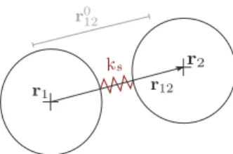
Fig. 1. Spring Model: linear spring to keep constant the inter-particle distance.

Fig. 2. Joint Model: overlapping due to bending if no gap between beads.

Fig. 3. Joint Model: c1is separated by a gapεgfrom the beads.

order. The latteris thecornerstone which differentiates previous works inthe literature fromours. Numerous strategies havebeenemployedtohandlekinematicconstraints.

[32,34,35,40]and[50]usedalinearspringtomodeltheresistancetostretchingandcompressionwithoutanyconstraint

onthebeadrotationalmotion(Fig. 1).Theresultingstretchingforcereads:

Fs

= −

ks

¡

ri,i+1

−

r0i,i+1

¢

(1) where

•

ksisthespringstiffness,

•

ri,i+1

=

ri+1

−

ri isthedistancevectorbetweentwoadjacentbeads(forsimplicity,equationsandfigureswillbe

pre-sentedforbeads1 and2 andcaneasilybegeneralizedtobeadsi andi

+

1),

•

r0_1,2isthevectorcorrespondingtoequilibrium.

However, regarding the connectivity constraint, the spring model is somehow approximate. A linear spring is prone touncontrolled oscillationsandthe problemmaybecomeunstable. Manyother authors,amongwhich [28–30],thus use non-linear spring models for a better description of polymer physics. Nevertheless, the repulsive force stiffness has an importantnumericalcostintime-steppingaswillbediscussedinSection2.6.3.Furthermore,unconstrainedbeadrotational motionleadstospurioushydrodynamicinteractionsandthuslimitstherangeofapplicationsfortheseBM.

Alternatively, [47–49,53] and [46] constrained the motion of the beads such that the contact point for each pair ci

remainsthesame.Whilemorerepresentativeofaflexibleobject,thisapproachexhibitstwomaindrawbacks: 1. agapbetweenbeadsisnecessarytoallowtheobjecttobend(seeFig. 2),

2. itrequiresan additionalcentertocenterrepulsive force,andthusmoretuningnumericalparameters toprevent over-lappingbetweenadjacentbeads.

Consider two adjacent beads, withradius a, linked by a hinge c1 (typicallycalled ball andsocket joint). The gap

ε

g

definesthedistancebetweenthespheresurfacesandthejoint(seeFig. 3).Denotepithevectorattachedtobeadi pointing

towardsthenextjoint,i.e.thecontactpointci.

Theconnectivitybetweentwocontiguousbodieswrites:

£

r1

+ (

a

+

ε

g

)

p1

¤ − £

r2

− (

a

+

ε

g

)

p2

¤ =

0 (2)

anditstimederivative

˙

ri and

ω

i arethe translationalandrotational velocitiesofbeadi. Theconstraintforcesandtorques associatedto (3)are

obtainedeitherbysolvingalinearsystemofequationsinvolvingbeadsvelocities[53],orbyinserting(3)intotheequations ofmotionwhenneglectinghydrodynamicinteractions[48,49].

The gap width 2

ε

g controls the maximumcurvature

κ

maxJ allowed without overlapping. From the sine rule, one can

derive thesimpleequationrelating

ε

g and

κ

maxJ

κ

maxJ

=

q

1

− (

_a+a_ε g

)

2 a (4)

Onceawareoftheselimitations,thegap

ε

g,rangeandstrengthoftherepulsiveforce shouldbe prescribeddependingon

theproblemtobeaddressed.

[56] and[43] proposedamoresophisticatedJointModelthan thosehithertocited,usingafulldescriptionofthelinks dynamicsalongthecurvilinearabscissa.Theyderivedasubtleconstraintformulationwhichensuresthatthetangentvector tothecenterlineiscontinuousandthatthelengthoflinksremainsconstant.Thesetwoworksareworthmentioningsince they avoidan empiricaltuning ofrepulsiveforces.Yet, [56]computedthe constraintforcesandtorqueswithan iterative penaltyschemeinsteadofusinganexplicitformulation.

Finally,itisworthmentioningthatthebeadmodelproposedin[31]circumventstheinextensibilitydifficultyby impos-ingconstraintsontherelativevelocitiesofeachsuccessivesegments,sothattheirrelativedistanceiskept constant.Using bendingpotential,[31]permitoverlapbetweenbeadswithrestoringtorque(cf.Fig. 2).ALagrangianmultiplierformulation oftensileforcesis alsousedin[57],whichisequivalentto aprescribed equaldistancebetweensuccessivebeads.Again, inextensibilityconditiondoesnotpreventbeadoverlappingduetobendinginthisformulation.Thecomputationofcontact forceswhichisproposedinthefollowingSection2.2generalizestheLagrangianmultiplierformulationof[31]to general-izedforces.Usingmorecomplexconstraintsinvolvingbothtranslationalandangularvelocities,weshowthatitispossible toaccommodate bothnon-overlappingandinextensibilityconditionswithoutadditionalrepulsiveforces(usingtherolling no-slipcontactwiththegearsmodeldetailedinSection2.3).Thisproposedgeneralformulationisalsowellsuitedforany typeofkinematicboundaryconditionsasillustratedinSection3.4.

2.2. Generalizedforces,virtualworkprincipleandLagrangemultipliers

ThemodelandformalismproposedinthisarticlerelyonearlierworkinAnalyticalMechanicsandRobotics[58,59].The conceptofgeneralizedcoordinatesandconstraintswhichhasproventobeveryusefulinthesecontextsisdescribedhere. Generalizedcoordinates refer toa setofparameters whichuniquely describestheconfigurationofthe systemrelativeto some referenceparameters (positions,angles,. . . ).Fordescribingobjectsofcomplexshape,let usconsiderthepositionri

ofeach beadi

∈ {

1

,

Nb

}

withassociatedorientation vector pi whichis definedby threeEulerangles p

≡ (θ,

φ,

ψ )

. Inthe

following, anycollectionofvector population

(

r1

,

..

ri

,

..

rNb

)

≡

R willbe capitalized,so that R isa vector in

R

3Nb_.Hence the collection of orientation vectors pi will be denoted P, which is a vector of length 3Nb, the collection of velocities

dri

dt

= ˙

ri

=

vi, will be denoted V, the collection of angular velocity p

˙

i

≡

ω

i will be

Ä

, the collectionof forces fi, F, the

collectionoftorques

γ

_i,

Γ

.AllV,

Ä

,F and

Γ

arevectorsin

_R

3Nb_.

Let usthen define some generalized coordinateqi foreach bead, which isdefined by qi

≡ (

ri

,

pi

)

≡ {

r1,i

,

r2,i

,

r3,i

,

θ

i

,

φ

i

,

ψ

i

}

sothatthecollectionofgeneralizedpositions

(

q1

,

..

qi

,

..

qNb

)

≡

Q isavectorin

R

6Nb_{.Generalizedvelocitiesarethen} definedbyvectorsq

˙

i

≡ (

vi

,

ω

i

)

withassociatedgeneralizedcollectionofvelocitiesQ.

˙

Articulated systems aregenerically submitted to constraintswhich areeither holonomic,non-holonomicorboth [33]. Holonomic constraintsdonot dependonanykinematicparameter(i.eanytranslational orangularvelocity)whereas non-holonomicconstraintsdo.

In thefollowing we considernon-holonomic linearkinematicconstraints associatedwithgeneralized velocitiesofthe form[60]

J

J

J

Q

˙

+

B

=

0

,

(5)

such that

J

J

J

is a 6Nb

×

Nc matrix andB is avector of Nc components. Nc isthe numberof constraintsacting on the

Nb beads.B and

J

J

J

mightdepend (even non-linearly)ontime t andgeneralizedpositions Q,butdonotdepend onany

velocityofvector_Q,

˙

sothatrelation(5)islinearin_Q.

˙

Insubsequentsections,weprovidespecificexamplesforwhichthis class ofconstraints areuseful. Here we describe,following [58,60] howsuch constraints canbe handled thanksto some generalizedforcethatcanbedefinedfromLagrangemultipliers.Theideaformulatedtoincludeconstraintsinthedynamics of articulatedsystems isto search additional forceswhich could permit to satisfy these constraints.First, one mustrely on generalizedforces

f

i

≡ (

fi

,

γ

i

)

whichincludeforcesandtorques actingoneach bead, whosecollection

(f

1

,

f

i

,

..f

Nb

)

is denoted

F

.Generalizedforcesaredefinedsuchthatthe totalworkvariation

δ

W isthescalarproductbetweenthemand thegeneralizedcoordinatesvariations

δ

Q

sothat,ontherighthandside of(6)onealsogetsthetranslationalandtherotationalcomponentsofthework.Then,the ideaofvirtualworkprincipleistosearchsomevirtualdisplacement

δ

Q thatwillgeneratenowork,sothat

F · δ

Q

=

0. (7)

Atthesametime,byrewriting(5)indifferentialform

J

J

J

dQ

+

Bdt

=

0

,

(8)

admissiblevirtualdisplacements,i.e. thosesatisfyingconstraints(8),shouldsatisfy

J

J

J

δ

Q

=

0

.

(9)

Combiningthe Nc constraints(9)with(7)ispossibleusinganylinearcombinationoftheseconstraints.Suchlinear

com-binationinvolves Nc parameters,theso-calledLagrangemultiplierswhicharethe componentsofa vector

λ

in

R

Nc.Then

fromthedifferencebetween(7)andthe Nc linearcombinationof(9)onegets

(F − λ ·

J

J

J

) · δ

Q

=

0. (10)

Prescribinganadequateconstraintforce

F

c

= λ ·

J

J

J

,

(11)

permitstosatisfy therequiredequalityforanyvirtualdisplacement.Hence,theconstraintscanbehandledbyforcing the dynamicswithadditionalforces,theamplitudeofwhicharegivenbyLagrangemultipliers,yettobefound.Notealso,that thisfirst result impliesthat both translational forcesand rotationaltorques associatedwith the Nc constraints are both

associatedwiththesameLagrangemultipliers.

ThisformalismisparticularlysuitableforlowReynoldsnumberflowsforwhichtranslationalandangularvelocitiesare linearlyrelatedtoforcesandtorquesactingonbeadsbythemobilitymatrixM

µ

V

Ä

¶

=

M

µ

F

Γ

¶

+

µ

V∞

Ä

∞

¶

+

C

:

E∞

.

(12) V∞

= (

v∞₁

,

. . . ,

v∞_Nb

)

and

Ä

∞

= (

ω

∞

1

,

. . . ,

ω

∞Nb

)

correspondtothe ambientflowevaluated atthecentersof massri. E

∞ _is

therateofstrain3

×

3 tensoroftheambientflow.C isathirdranktensorcalledthesheardisturbancetensor,itrelatesthe particlesvelocitiesandrotationstoE∞ [54].MatrixM (andtensorC)canalsobere-organizedintoageneralizedmobility matrix

M

M

M

(generalizedtensor

C

C

C

resp.)inorderto define thelinearrelation betweenthepreviously definedgeneralized velocityandgeneralizedforce

˙

Q

=

M

M

M

F +

V

V

V

∞

+

C

C

C

:

E∞

,

(13)

where

V

V

V

∞

_{= (}

_v∞

1

,

ω

∞1

,

. . . ,

v∞Nb

,

ω

∞

Nb

)

.TheexplicitcorrespondencebetweentheclassicalmatrixM andtheherebyproposed generalized coordinate formulation

M

M

M

is given in Appendix A. Hence, as opposed to the Euler–Lagrange formalism of classical mechanics,the dynamics oflow Reynolds numberflows doesnot involve anyinertialcontribution, andprovide a simple linear relationship between forces and motion. In this framework, it is then easy to handle constraints with generalizedforces,becausethetotalforce willbethe sumoftheknownhydrodynamic forces

F

h,elasticforces

F

e,inner

forces associated to active fibers

F

a and the hereby discussed and yet unknown contact forces

F

c to verify kinematic

constraints

F = F

′

_{+ F}

c

,

with (14)

F

′

_{= F}

h

+ F

e

+ F

a

.

(15)

Hence,ifoneisabletocomputetheLagrangemultipliers

λ

,thecontactforceswillprovidethetotalforcebylinear su-perposition(14),whichgivesthegeneralizedvelocitieswith(13).Now,letusshowhowtocomputetheLagrangemultiplier vector.Sincethegeneralizedforce isdecomposedintoknownforces

F

′ _{andunknowncontactforces}

_F

_c

_{= λ ·}

_J

_J

_J

_,relations

(14)and(13)canbepooledtogetheryielding

M

M

M

F

c

=

M

M

M

λ

J

J

J

= ˙

Q

−

M

M

M

F

′

−

V

V

V

∞

−

C

C

C

:

E∞

.

(16) Sothat,using(5),

J

J

J M

M

M J

J

J

T

λ = −

B

−

J

J

J

¡

M

M

M

F

′

+

V

V

V

∞

+

C

C

C

:

E∞

¢,

(17)

Fig. 4. Gears Model: contact velocity must be the same for each bead (no-slip condition).

2.3. TheGearsModel

TheEuler–Lagrangeformalismcanbereadilyappliedtoanytypeofnon-holonomicconstraintsuchas(3).Inthe follow-ing,weproposeanalternativemodelbasedonno-slipconditionbetweenthebeads:theGearsModel.Thisconstraint,first introducedinaBeadModel(BM)by[27],convenientlyavoidnumericaltrickssuchasartificialgapsandrepulsiveforces.

However, [27] and [61] relied on to an iterative procedure to meet requirements. Here, we use the Euler–Lagrange formalismtohandlethekinematicconstraintsassociatedtotheGearsModel.

Consideringtwoadjacentbeads(Fig. 4),thevelocityvc1 atthecontactpointmustbethesameforeachsphere:

v1_c1

−

v2_c1

=

0

.

(18)

vL_c1 andvR_c1 are respectively therigid body velocity atthe contactpoint onbead1 andbead2. Denote

σ

1 _{the vectorial}

no-slipconstraint.(18)becomes

σ

1

(˙

r1

,

ω

1

, ˙

r2

,

ω

2

) =

0

,

(19)

i.e.

[˙

r1

−

ae12

×

ω

1

] − [˙

r2

−

ae21

×

ω

2

] =

0

,

(20)

where e12 isthe unitvector connectingthe centerofbead1,locatedatr1,to thecenterofbead2,located atr2 (e12

=

e2

−

e1).Theorientationpi vectorattachedtobeadi,isnotnecessarytodescribethesystem.Hence,from(20)onerealizes

that

σ

1 _{islinearintranslationalandrotationalvelocities.ThereforeEq.(19)canbereformulatedas}

σ

1

( ˙

Q

) =

J1Q

˙

=

0

,

(21)

where,Q is

˙

thecollectionvectorofgeneralizedvelocitiesofthetwo-beadassembly

˙

Q

= [˙

r1

,

ω

1

, ˙

r2

,

ω

2

]

T

,

(22)

J1 istheJacobianmatrixof

σ

1_:

J_kl1

=

∂

σ

1 k

∂

Ql

,

k

=

1, . . . ,3,l

=

1, . . . ,12, (23) J1

=

£

J1₁ J1₂

¤ = £

I3

−

ae×₁₂

−

I3 ae×₂₁

¤ ,

(24) and e×

=





0

−

e3 e2 e3 0

−

e1

−

e2 e1 0





.

(25)

ForanassemblyofNbbeads,Nb

−

1 no-slipvectorialconstraintsmustbesatisfied.TheGearsModel(GM)totalJacobian

matrix

J

GMisblockbi-diagonalandreads

J

GM

=













J1₁ J1₂ J2₂ J2₃

. .

_.

. .

_.

JNb−1 Nb−1 J Nb−1 Nb













(26)

whereJα_β isthe3

×

6 Jacobianmatrixofthevectorialconstraint

α

forthebead

β

. Thekinematicconstraintsforthewholeassemblythenread

J

GMQ

˙

=

0

.

(27)

Fig. 5. Beamdiscretizationandbendingtorquescomputationofbeads1,3and5.Remainingtorquesareaccordinglyobtained:γb

2=m(s3)andγb4=

−m(s3).

2.4.Elasticforcesandtorques

Weareconsideringelastohydrodynamics ofhomogeneousflexibleandinextensiblefibers.Theseobjectsexperience bend-ing torques and elastic forces to recover their equilibrium shape. Bending moments derivation and discretization are provided.Then, the role ofbending moments andconstraintforces isaddressed inthe force andtorque balance forthe assembly.

2.4.1. Bendingmoments

Thebendingmomentofanelasticbeamisprovidedbytheconstitutivelaw[55,62] m

(

s

) =

Kbt

×

dt

ds

,

(28)

whereKb

₍

_s

₎

_{isthebendingrigidity,t isthetangentvectoralongthebeamcenterlineands isthecurvilinearabscissa.Using}

theFrenet–Serretformula

dt

ds

=

κ

n

,

(29)

thebendingmomentwrites

m

(

s

) =

Kb

κ

b

,

(30)

where

κ

(

s

)

definesthelocalcurvature,n

(

s

)

andb

(

s

)

arethenormalandbinormalvectorsoftheFrenet–Serretframe.When thelinkconsideredisnotstraightatrest,withanequilibriumcurvature

κ

eq

₍

_s

₎

_{,(30)ismodifiedinto}

m

(

s

) =

Kb

¡

κ

−

κ

eq

¢

b

.

(31)

Here,thebeamisdiscretizedintoNb

−

1 rigidrodsoflengthl

=

2a (cf.Fig. 5).Inextensiblerodsaremadeupoftwobond

beadsandlinked together bya flexible jointwithbendingrigidity Kb.Bendingmoments are evaluatedatjointlocations si

= (

i

−

1

)

l fori

=

2

,

. . . ,

Nb

−

1,wheresicorrespondtothecurvilinearabscissaofthemasscenteroftheithbead.

Thebendingtorqueonbeadi isthengivenby

γ

b_i

=

m

(

si+1

) −

m

(

si−1

),

(32)

withm

(

si

)

=

Kb

κ

(

si

)

b

(

si

)

.SeeFig. 5forthetorquecomputationonabeamdiscretizedwithfourrods.

Thelocalcurvature

κ

(

si

)

isapproximatedusingthesinerule[42]

κ

(

si

) =

1 a

r

1

+

ei−1,i

.

ei,i+1 2 (33)

whereei−1,i istheunitvectorconnectingthecenterofmassofbeadi

−

1 tothecenterofmassofbeadi.Thiselementary

geometriclawprovidestheradiusofcurvature R

(

si

)

=

1

/

κ

(

si

)

ofthecirclecircumscribingneighboring beadcentersri−1,ri

andri+1.

Amore generalversion of thediscrete curvature proposed in[63] canalso be used inthe caseofthree dimensional motion.Inthatcase,thecurvatureofthefiberisdiscretizedasin[63]

κ

(

si

) =

ei−1,i

×

ei,i+1

where, again, ei−1,i is the unit vector connectingthe centerof massof beadi

−

1 to thecenter ofmass ofbead i.The

bendingmomentreads

m

(

si

) =

Kb

κ

(

si

).

(35)

Toincludetheeffectoftorsionaltwistingabout theaxisofthefiber,one wouldhaveto computethe relativeorientation between the framesof reference attachedto the beads using Euler angles [56] (see Section 2.2) or unit quaternions as in [53].This wouldprovidethe rateof changeofthe twistanglealong thefiber centerlineandthus thetwisting torque actingoneachbead.Inthefollowing,onlybendingeffectsareconsidered.

2.4.2. Forceandmomentactingoneachbead

TheGearsModelproposedinthispaperdoesnotneedtoconsidergapstoallowbending.

F

c alsoensuresthe

connectiv-ityconditionandcircumventtheuseofrepulsiveforcesasdistancesbetweenadjacentbeadsurfacesremainconstant.More specifically, thetangential componentsof theforce Fc,whichis onlyone partofthegeneralized force

F

c,actsastensile

force.

Foreachbeadi,contactforcesappliedfrombeadi tobeadi

+

1 atcontactpointcibetweenbeadi andi

+

1 (Fig. 4for

twobeads)isdenotedfci.FromNewtonthirdlawatcontactpointci,thecontactforceappliedtobeadi frombeadi

+

1 is obviously

−

fci.Totalforceactingonbeadi fromcontact,andhydrodynamicforcesf

h i reads

fi

=

fci−1

−

fci

+

f

h

i (36)

Similarly,thecontactforcefci atpointci producesamomentmci

=

ati

×

fci associatedwithlocaltangentvectorti

=

ei,i+1 anddistancea to the neutralfiberatpoint ci.Totalmomentacting onbeadi from contactpoints moments, elasticand

hydrodynamictorquesarethen

γ

i

=

mci−1

−

mci

+

γ

b

i

+

γ

hi

.

(37)

The contributionofcontactforceandcontactmomentactingonbeadi exactly equalsthecontributionofthegeneralized contactforce.Indeed,usingthekinematicconstraintsJacobian(26)in(11),andcomputingtheforceandtorque contribu-tions, one exactlyrecovers thefirst andthesecond contributions oftheright-hand-sideof(36) and(37). InAppendix B, wealsoshowthatthismodelisconsistentwithclassicalformulationforslenderbodyforceandmomentbalancewhenthe beadradiustendstozero.

2.5. Hydrodynamiccoupling

Movingobjects(rigidorflexiblefibers)inaviscousfluidexperiencehydrodynamicforcing.Theinteractionsaremediated bythefluidflowperturbationswhichcanalterthemotionandthedeformationofthefibersinamoderatelyconcentrated suspension. Theexistenceofhydrodynamicinteractions hasalsoan effectona singlefiberdynamicswhiledifferentparts ofthefibercanrespondtotheambientflowbutalsotolocalflowperturbationsrelatedtothefiberdeformation.Resistive ForceTheory(RFT)canbeusedtoestimatethefiberresponsetoagivenflowassumingthatthefiberismodeledbyalarge seriesofslenderobjects[23,64].Slenderbodytheoryhasalsobeenused[20,65]torelatelocalbalanceofdrag forceswith the filamentforcesupon thefluid resultingina dynamicalsystemto modelthedeformation ofthefibercenterline.This modelprovidedinterestingresultsonthestretch-coiltransitionoffibersinvorticalflows.

Inourbeadsmodel,thefiberiscomposedofsphericalparticlestoaccountforthefinitewidthofitscross-section.The hydrodynamic interactions areprovidedthrough thesolutionofthemobilityproblemwhichrelatesforces,torquesto the translational and rotationalvelocities ofthe beads.Thismany-body problemisnon-linear in theinstantaneous positions of all particles ofthe system. Approximate solutions of thiscomplex mathematicalproblem canbe achieved by limiting the mobility matricesto their leading order. The simplest model iscalled free drain as themobility matrix is assumed to be diagonalneglecting the HIwith neighboring spheres.Pairwise interactions are requiredto account foranisotropic drag effects within the beadscomposing thefiber. The Rotne–Prager–Yamakawa(RPY) approximation is one ofthe most commonlyusedmethodsofincludinghydrodynamicinteractions.Thiswidelyusedapproachhasbeenrecentlyupdatedby Wajnrybetal.[54]fortheRPYtranslationalandrotationaldegreesoffreedom,aswellasforthesheardisturbancetensor C whichgivestheresponseoftheparticlestoanexternalshearflow(12).

2.6. Numericalimplementation 2.6.1. Integrationschemeandalgorithm

The kinematicsofthe constrainedsystemresultsfromthesuperpositionofindividual beadmotions.Positionsare ob-tainedfromthetemporalintegrationoftheequationofmotionwithathirdorderAdams–Bashforthscheme

dri

dt

=

vi

,

(38)

Thetimestep

1

t usedtointegrate(38)isfixedbythecharacteristicbendingtime[46]

1

t

<

µ

(2a)

4

Kb

,

(39)

where

µ

isthesuspendingfluidviscosity.

Theevaluationofbeadinteractionsmustfollowaspecificorder.Elasticandactiveforcescanbecomputedinanyorder. Constraintforcesandtorquesmustbeestimatedafterwardsastheydependon

F

′.Thenvelocitiesandrotationsareobtained fromthemobilityrelation.Andfinally,beadpositionsareupdated.

•

Initialization:positionsri

(

0

)

,

•

TimeLoop

1. Evaluatemobilitymatrix

M (

Q

)

and

C :

E∞_{(seeSection2.5),}

2. Calculatelocalcurvatures(33)andbendingtorques

γ

b

i (32)toget

F

e,

3. Addactiveforcing

F

aandambientvelocity

V

∞ ifany,

4. ComputetheJacobianmatrixassociatedwithnon-holonomicconstraints

J (

Q

)

, 5. Solve(17)togettheconstraintforces

F

c

= λ

J

,

6. Sumalltheforcingterms

F

= F

e

+ F

a

+ F

c,

7. Applymobilityrelation(13)toobtainthebeadvelocities_Q,

˙

8. Integrate(38)togetthenewbeadpositions.

2.6.2. ImplementationoftheJointModel

Toprovideacomprehensivecomparisonwithpreviousworks,weexploittheflexibilityoftheEuler–Lagrangeformalism toimplementtheJointModelasdescribedin[49] supplementedwithhydrodynamicinteractions. Thejointconstraintfor twoneighboring beadsreads

£˙

ri

− (

a

+

ε

g

)

pi

×

ω

i

¤ − £˙

ri+1

+ (

a

+

ε

g

)

pi+1

×

ω

i+1

¤ =

0

.

(40)

UsingtheEuler–Lagrangeformalism,(40)isreformulatedwiththeJointModel(JM)Jacobianmatrix

J

JMQ

˙

=

0

,

(41)

where

J

JMhasthesamestructureasin(26)and

Ji

=

£

Ji₁ J₂i

¤ = £

I3

−(

a

+

ε

g

)

p×_i

−

I3

−(

a

+

ε

g

)

p×_i+1

¤ .

(42)

Accordingly,thecorrespondingsetofforcesandtorques

F

c areobtainedfromSection 2.2.AsmentionedinSection 2.1,

suchformulationdoesnotpreventbeadsfromoverlappingwhenbendingoccurs.ArepulsiveforceFrisaddedaccordingto

[46](theforceprofileproposedby[49]isverystiff,thusveryconstrainingforthetimestep):

Fr_{i j}

=















−

F0exp(−di j_d+δD 0

)

ei j

,

di j

≤ −δ

D

,

−

F0

(

1₂

−

₂d_δi j_D

)

ei j

,

−δ

D

<

di j

≤ δ

D

,

0

,

ri j

> δ

D

.

(43)

δ

D isan artificial surface roughness, di j isthe surface to surface distance.di j

<

0 indicatesoverlapping betweenbeads i

and j.d0 isa numericaldampingdistancewhich hastobe tuned to preventoverlapping. F0 istherepulsive force scale

chosen inorder to avoidnumericalinstabilities. Todeal withthisissue,[46] proposed toevaluate F0 frombending and

viscousstresses.Aslightmodificationoftheirformulaforinertialessparticlesyields

F0

=

C16

π µ

L

¡

v∞

−

v

¢ +

C2

s

Kb_Eb

L3

,

(44)

the bar denotes the average over the constitutive beads or joints where C1 and C2 are adjustable constants. Eb is the

bendingenergy Eb

=

Nb−1

X

i=1 Kb

¡

κ

(

si

) −

κ

eq

(

si

)

¢

2

.

(45)

Bendingmomentsareevaluatedatthejointlocationss_iJ

= (

a

+

ε

g

)

+ (

i

−

1

)

×

2

(

a

+

ε

g

)

,i

=

1

,

. . . ,

Nb

−

1.Jointcurvature

isgivenby

κ

¡

s_iJ

¢ =

2 a

+

ε

g

r

1

+

pi

.

pi+1 2

.

(46)

Fig. 6. Dependenceoftheconstraintsǫ¯M/ ˙γL onthetimestepγ˙1t,+:GearsModel,1:JointModel.Inset:ǫ¯M/ ˙γL withtheGearsModelforafixedtime

step given by(39)for different values ofγ˙.

Similarlyto(32),bendingtorqueonbeadi is

γ

b_i

=

m

¡

s_iJ

¢ −

m

¡

s_iJ₋₁

¢.

(47)

Beadorientationpi isintegratedwithathirdorderAdams–Bashforthscheme

dpi

dt

=

ω

i

×

pi

.

(48)

TheprocedureissimilartotheGearsModel.piareinitializedtogetherwiththepositions.TherepulsiveforceFrisadded

to

F

′andcanbecomputedbetweenstep1and5oftheaforementionedalgorithm.Timeintegrationof(48)isperformed atstep8.

2.6.3. Constraintsandnumericalstability

At each time step, the error on kinematic constraints

ǫ

is evaluated, after application of the mobility relation (13), betweenstep7andstep8:

ǫ

GM

(

t

) =

°

°

J

GMQ

˙

°

°

2

=

Ã

Nb−1

X

i=1

¡

vL_c i

−

v R ci

¢

2

!

1/2 (49)

fortheGearsModel,and

ǫ

JM

(

t

) =

°

°

J

JMQ

˙

°

°

2 (50)

fortheJointModel.

ToverifytherobustnessofbothmodelsandLagrangeformulation,anumericalstudyiscarriedoutonastiff configura-tion.

Afiberofaspectratiorp

=

10 withbendingratioBR

=

0

.

01 isinitiallyalignedwithashearflowofmagnitude

γ

˙

=

5 s−1.

Forthisaspectratio,Nb

=

10 beadsareusedtomodelthefiberwiththeGearsModel.

JointModelinvolvesadditionalitemstobefixed.Nb

=

9 spheresareseparatedbyagapwidth2

ε

g

=

0

.

25a.Therepulsive

force isactivated whenthesurface to surfacedistancedi j reachesthe artificialsurfaceroughness

δ

D

=

2

(

a

+

ε

g

)/

10.The

remainingcoefficientsaresettoreducenumericalinstabilitieswithoutaffectingthePhysicsofthesystem:d0

= (

a

+

ε

g

)/

4,

C1

=

5 andC2

=

0

.

5.

Fig. 6 showsthe evolution ofthe maximal mean deviation fromthe no-slip/jointconstraint

ǫ

¯

M

=

maxt

ǫ

(

t

)/(

Nb

−

1

)

normalized withthe maximal shear velocity

γ

˙

L dependingon the dimensionless time step

γ

˙

1

t. First, one can observe thatforbothJointandGearsmodels,

ǫ

¯

M

/ ˙

γ

L weaklydependson

γ

˙

1

t andtheresultingmotionofthebeadscompliesvery

preciselywiththesetofconstraints,withinatoleranceclosetounitroundoff(

<

2

.

10−16_{).Secondly,JointModelisunstable}

fortime steps 100times smallerthan GearsModel.The onset fornumericalinstability indicates that therepulsive force stiffnessdominatesoverbending,thusdictatingandrestrictingthetimestep.

As acomparison, [46] matched connectivityconstraintswithin 1% errorforeach fibersegment.Todoso, theyhadto useaniterativeschemereducingthetimestepby1

/

3 eachiterationtomeetrequirementsandlimitoverlappingbetween adjacentsegments.Forsimilarresults,astiffconfiguration,suchastheshearedfiber,isthereforemoreefficientlysimulated withtheGearsModel.

Thirdly,insetofFig. 6showsthat,foragiventime step,theGearsModelconstraints

ǫ

¯

M

/ ˙

γ

L aresatisfiedwhateverthe

shearmagnitude.Hence,(39)ensuresunconditionallynumericalstabilityasbendingistheonlylimitingeffectfortheGears Model.

Hence,therobustnessoftheEuler–Lagrangeformalismandthenumericalintegrationwechoseprovideastrongsupport totheGearsModelovertheJointModel.

Asa final remarktothissection, itisimportantto mentionthat thenumericalcost oftheproposed methodstrongly dependsonthechoice forthemobilitymatrixcomputation,asusual forbeadmodels.Ifthemobilitymatrixiscomputed takingintoaccountfullhydrodynamicinteractionswithStokesianDynamics,mostofthenumericalcostwillcomefromits evaluationinthiscase.ThislimitationcouldbeovercameusingmoresophisticatedmethodssuchasAcceleratedStokesian Dynamics [66] orForce Coupling Method[18].Moreover, when considering Rotne–Prager–Yamakawa mobilitymatrix, its costonlyrequirestheevaluationof O

((

6Nb

)

2

)

terms.Furthermore,the mainalgorithmiccomplexityofbeadmodels does

not comefrom thetime integration ofthe beadpositions which only requiresa matrix–vector multiplication (13)at an O

((

6Nb

)

2

)

cost.Fast-multipoleformulationofaRotne–Prager–Yamakawamatrixcanevenprovidean O

(

6Nb

)

costforsuch

matrix–vectormultiplication[67].

Themain numericalcost indeedcomes fromtheinversion ofthecontactforces problem(17). Itis worth notingthat thislinearproblemis Nc

×

Nc whichisslightlydifferentfromNb

×

Nb,butofthesameorder.Furthermore,problem(17)

givesadirect,singlestepproceduretocomputethecontactforces,asopposedtopreviousotherattempts[27,46,56]which requirediterativeprocedurestomeetforcesrequirements,involvingthemobilitymatrixinversionateachiteration.Thecost fortheinversionof(17)liesin-between O

(

N2

c

)

andO

(

N3c

)

dependingontheinversionmethod. 3. Validations

3.1. Jefferyorbitsofrigidfibers

MuchofourcurrentunderstandingofthebehavioroffibersexperiencingashearflowhascomefromtheworkofJeffery

[68]whoderived theequationforthemotionofan ellipsoidalparticleinStokesflow.The sameequation canbeusedfor themotion ofan axisymmetric particle by using an equivalentellipsoidalaspect ratio.Rigid fibers can be approximated byelongated prolateellipsoids.Anisolated fiberinsimpleshearflow rotatesinaperiodicorbitwhilethecenterofmass simplytranslatesintheflow (nomigration acrossstreamlines). Theperiod T (51)is afunctionofthe aspectratioofthe fiberandtheflowshearratewhiletheorbitdependsontheinitialorientationoftheobjectrelativetotheshearplane

T

=

2

π

(

re

+

1/re

)

˙

γ

.

(51)

˙

γ

is the shearrate ofthe carryingflow. re is theequivalentellipsoidal aspect ratiowhich isrelated to thefiber aspect

ratio rp (lengthof the fiberover diameterof thecross-section which turns out to rp

=

Nb with Nb beads). The fiberis

initiallyplacedintheplaneofshearandiscomposedonNb beads.NogapsbetweenbeadsisrequiredintheJointModel

becausethefiberisrigidandflexibilitydeformationsarenegligible.Wehavecomparedtheresultswithtworelationsfor re:

Cox[1] re

=

1.24rp

p

ln(rp

)

,

(52) andLarson[69] re

=

0.7rp

.

(53)

Thisclassic andsimple test case hasbeen successfully validatedin [27,34,49]. Both the Joint andGears models give a correctpredictionof theperiod ofJeffery orbits(Fig. 7). The scaled period

γ

˙

T ofsimulations remains within the two evolutionsbasedonEqs.(52)and(53).Wehavetriedtocompareit withthelinearspringmodelproposed byGaugerand Stark[40](andusedbySlowickaetal.[50] witha moredetailedformulationofhydrodynamic interactions).Inthislatter model,thereisnoconstraintontherotationofbeadsandthesimulationsfailedtoreproduceJefferyorbits(thefiberdoes notflipovertheaxisparalleltotheflow).

3.2.Flexiblefiberinashearflow

Themotionofflexiblefibersinashearflowisessentialinpapermakingorcompositeprocessing.Predictionandcontrol offiberorientationsandpositionsare ofparticularinterest inthestudyofflocksdisintegration.Many modelshavebeen designedto predictfiberdynamicsandmuchexperimental workhasbeenconducted.Thewide varietyoffiberbehaviors dependson theratio ofbending stressesover shearstress, which isquantified by a dimensionless number,the bending ratioBR[53,70]

BR

=

E

(ln 2r

e

−

1.5)

µ

γ

˙

2r4p

(54)

Fig. 7. TumblingperiodT dependingonfiberaspectratiorp. :theoreticallaw(51)withregivenby(53), :theoreticallaw(51)withre givenby

(52),P: Gears Model,e: Joint Model.

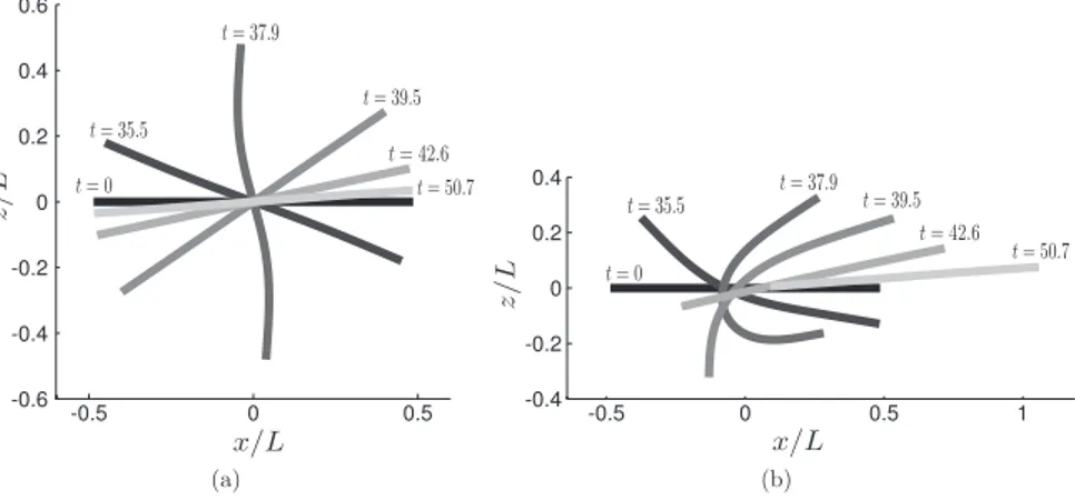
Fig. 8. OrbitofaflexiblefilamentinashearflowwithBR=0.04.Temporalevolutionisshownintheplaneofshearflow.(a) Symmetric“S-shape”ofa straightfilament,κeq_{=0.(b) Bucklingofapermanentlydeformedrodwithanintrinsiccurvatureκ}eq_=1/(100L).

Inthefollowing,weinvestigatetheresponseoftheGearsModelwithknownresultsonflexiblefiberdynamics. 3.2.1. Effectofpermanentdeformation

[70,71]analyzed the motionofflexiblethreadlikeparticles inashearflow dependingonBR. Theyobservedimportant

driftsfromtheJefferyorbitsandclassifiedthemintocategories.Yet,thegoalofthissectionisnottocarryoutanin-depth studyonthesephenomena.Instead,theobjectiveistoshowthatourmodelcanreproducebasicfeaturescharacteristicof shearedflexiblefilaments.Weanalyzefirsttheinfluenceofintrinsicdeformationonthemotion.

Ifa fiberisstraight atrest,it willsymmetricallydeform ina shearflow. When alignedwiththecompressive axesof the ambient rateof strain E∞, the fiber adoptsthe “S-shape” observed in Fig. 8(a). When aligned withthe extensional axes, tensile forces turn the rod back to its equilibrium shape. This symmetry is broken when the filament is initially slightly deformedor hasa permanent deformation atrest,i.e. a nonzeroequilibrium curvature

κ

eq

_>

_{0. An initial small}

perturbation of the shape of a straight filament aligned withflow can induce large deformations duringthe orbit. This phenomenonisknownasthebucklinginstabilitywhoseonsetandgrowtharequantifiedwithBR[72,73].Fig. 8(b)illustrates the evolution of a flexible sheared filament with BR

=

0

.

04 and a very small intrinsic deformation

κ

eq

₌

₁

_/(

_100L

₎

_.The

equilibriumdimensionlessradiusofcurvatureis2Req

/

L

=

200.Duringthetumblingmotionitdecreasestoaminimalvalue of2Rmin

/

L

=

0

.

26.Bucklingthusincreasesby770timesthemaximalfibercurvature.

3.2.2. Maximalfibercurvature

[74]measuredtheradiusofcurvature R ofshearedfiberforaspectratiosrp rangingfrom283to680.Theyreportedon

theevolutionoftheminimalvalue Rmin,i.e.themaximalcurvature

κ

max,withBR.[53] usedtheJointModelwithprolate

spheroidsbutnohydrodynamicinteractionsandcomparedtheirresultswith[74].Bothexperimentalresultsfrom[74]and simulationsfrom[53]areaccuratelyreproducedbytheGearsModel.

Hydrodynamicinteractionsbetweenfiberelementsplayanimportantroleinthebendingofflexiblefilaments[46,50,74]. AsmentionedinSection2.5theuseofspherestobuildanyarbitraryobjectiswellsuitedtocomputethesehydrodynamic interactions.However,modeling rigidslenderbodiesinastrongshearflowbecomescostlywhenincreasingthefiberaspect ratio.First,the aspectratioofafibermadeup of Nb spheresisrp

=

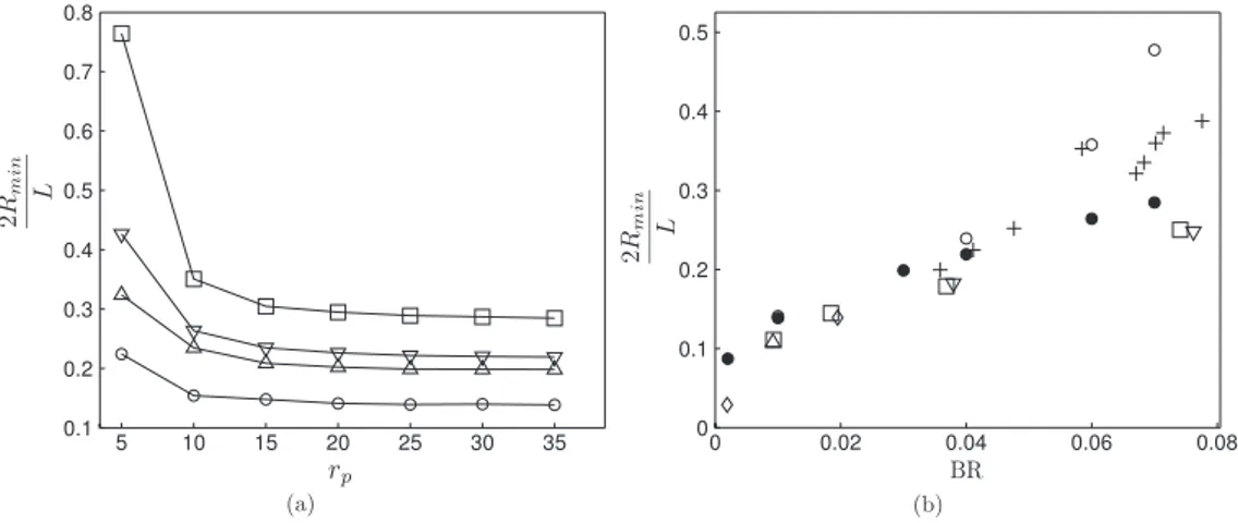
Nb.Eachtimeiteration requiresthecomputation of

Fig. 9. (a)Minimalradiusofcurvaturedependingonfiberlengthforseveralbendingratios. :BR=0.01, :BR=0.03, :BR=0.04, :BR

=0.07.(b) MinimalradiusofcurvaturealongBR.!:currentsimulationswithaspectratiorp=35 andintrinsiccurvatureκeq=0;":currentsimulations

with aspect ratio rp=35 and intrinsic curvatureκeq=1/(10L); simulation results from[53]withκeq=1/(10L): (E: rp=50,P: rp=100,e: rp=150,

1: rp=280);+: experimental measurements from[74], rp=283.

M

and

_{C :}

E∞ andtheinversionofalinearsystem(17)correspondingto Nc relationsofconstraintswithNc

≥

3

(

Nb

−

1

)

.

Secondly,foragivenshearrate

γ

˙

andbendingratioBR,Young’s modulus increasesasr4

p.Accordingto(39),thetimestep

becomesverysmallforlarge E. [53] partiallyavoidedthisissueby neglectingpairwise hydrodynamic interactions(

M

is diagonal),andbyassemblingprolatespheroidsofaspectratiosre

∼

10.

Yet, it is shown in Fig. 9(a) that for a fixed BR, 2Rmin

/

L converges asymptotically to a constant value with rp. An

asymptoticregime(relativevariationlessthan2%)isreachedforrp

≥

25.Choosingrp

=

35 thusenablesavalidcomparison

withpreviousresults.

Oursimulationresultscomparewellwiththeliteraturedata(Fig. 9(b))andbettermatchwithtoexperimentsthan[53]. When BR

≥

0

.

04, the Gears Model clearly underestimates measurements for

κ

eq

₌

₁

_/(

_10L

₎

_{and overestimates them for}

κ

eq

₌

_{0.However,SalinasandPittman[74]indicatedthattheerrorquantificationonparametersandmeasurementsis}

diffi-culttoestimateasthefiberswerehand-drawn.Notably,drawingaccuracydecreasesforlargeradiiofcurvature,whichleads totheconclusionthattheherebyobserved discrepancymightnotbe critical.Theydidnotreport thevalueofpermanent deformation

κ

eq _{forthefibersthey designed,whereas, asevidenced by[71],ithasastrongimpact on R}

min.Anumerical

studyofthisdependenceshouldbeconductedtocomparewith[71,Fig. 7].

[46]usedthesameapproachas[53]withhydrodynamicinteractions torepeatnumericallytheexperimentsfrom[74]; buttheirresults,thoughreliable,weredisplayedsuchthatdirectcomparisonwithpreviousworkisnotpossible.

Toconclude, it should be notedthat, in [53], the aspect ratiodoesnot affect 2Rmin

/

L for a fixed BR, confirmingthe

asymptoticbehaviorobservedinFig. 9(a). 3.3.Settlingfiber

ConsiderafibersettlingunderconstantgravityforceF⊥

=

F⊥e⊥ actingperpendicularlytoitsmajoraxis.Thedynamics

ofthesystemdependsonthree competingeffects:the elasticstresseswhich tendto returntheobjectto itsequilibrium shape,thegravitationalaccelerationwhichuniformlytranslatestheobjectandthehydrodynamicinteractionswhichcreates localdragalongthefilament.After atransient regime,thefilamentreachessteadystateandsettlesataconstantvelocity withafixedshape(seeFigs. 10(a)and 10(b)).Thissteadystatedependsontheelasto-gravitationalnumber

B

=

F⊥L

/

Kb

.

(55)

[41,75]and[65]examinedthecontributionofeachcompetingeffectbymeasuringthenormaldeflectionA,i.e.thedistance

betweentheuppermostandthelowermostpointofthefilamentalongthedirectionoftheapplied force(Fig. 10(b)); and thenormalfriction coefficient

γ

⊥

/

γ

⊥0 asa function of B.

γ

0

⊥ isthenormalfriction coefficient ofa rigidrod.To compute

hydrodynamicinteractions[75]usedStokeslet;[41],theForceCouplingMethod(FCM)[18];[65],SlenderBodyTheory. SimilarsimulationswerecarriedoutwithboththeJointModeldescribedinSection2.6.2andtheGearsModel.Fiberof length L

=

68a ismadeout of Nb

=

31 beadswithgapwidth 2

ε

g

=

0

.

2a for theJoint Modeland Nb

=

34 for theGears

Model.ToavoidbothoverlappingandnumericalinstabilitieswiththeJointModel,thefollowingrepulsiveforcecoefficients wereselected:d0

= (

a

+

ε

g

)/

4,

δ

D

= (

a

+

ε

g

)/

5,C1

=

0

.

01 and C2

=

0

.

01.NoadjustableparametersarerequiredforGears

Model.

Fig. 11 showsthat our simulations agreeremarkably well withprevious results exceptslight differenceswith[65] in

the linearregime B

<

100.Using SlenderBody Theory,[65] madethe assumption of a spheroidal filament instead of a cylindricalone,withaspectratiorp

=

100,i.e. threetimeslarger thanother simulations,whence suchdiscrepancies. The

Fig. 10. Shapeofsettlingfiberfor B=10000 intheframemovingwiththecenterofmass(xc,zc).(a)Metastable“W”shape,t=12L/Vs.(b)Steady

“horseshoe” shape at t=53L/Vs. Vsis the terminal settling velocity once steady state is reached.

Fig. 11. (a)ScaledverticaldeflectionA/L dependingonB. :GearsModel, :JointModel, :FCMresultsfrom[41], :Stokesletsresultsfrom

[75], :Slenderbodytheoryresultsfrom[65].(b)Normalfrictioncoefficientvs. B. :GearsModel, :JointModel, :FCMresultsfrom[41], :Stokesletsresultsfrom[75].

normalfriction coefficient (Fig. 11(b)),resultingfromhydrodynamic interactions, perfectlymatchesthe valueobtainedby

[41] withtheForce CouplingMethod.The FCMis knowntobetter describemultibody hydrodynamicinteractions. Sucha resultthussupportstheuseofthesimpleRotne–Prager–Yamakawatensorforthishydrodynamicsystem.

DifferencesbetweenGearsandJointModelsimplementedherearequantifiedbymeasuringtherelativediscrepancieson theverticaldeflection A

ǫ

A

=

AG

−

AJ

AG

,

(56)

andonthenormalfrictioncoefficient

γ

⊥

/

γ

⊥0

ǫ

γ⊥

=

(

γ

⊥

_/

_γ

⊥ 0

)

G

− (

γ

⊥

_/

_γ

⊥ 0

)

J

(

γ

⊥

_/

_γ

⊥ 0

)

G

.

(57)

DiscrepanciesbetweenJointandGearsmodelsremainbelow5% exceptatthethresholdofthenon-linearregime(B

≈

100)where

ǫ

A reaches15% and

ǫ

γ⊥

≈

7

.

5%.

Inaccordance with[75], a metastable “W”shape is reachedfor B

>

3000 (Fig. 10(a)) until it convergesto the stable “horseshoe”state(Fig. 10(b)).

3.4.Actuatedfilament

Thegoalofthefollowingsectionsistoshowthatthemodelweproposedisnotonlyvalidforpassiveobjectsbutalsofor activeones.Elastohydrodynamics alsoconcernswimmingatlowReynoldsnumber[6].Manytypeofmicro-swimmershave beenstudiedbothfromtheexperimentalandtheoreticalpointofview.Amongthemtwocategoriesaredistinguished: cili-atesandflagellates.Ciliatespropelthemselvesbybeatingarraysofshorthairs(cilia)ontheirsurfaceinasynchronizedway (Opalina,Volvox,Paramecia). Flagellatesundulate and/orrotatetheir externalappendageto push(pull)thefluid fromtheir aft(fore)part(spermatozoa,ChlamydomonasRheinardtii,BacillusSubtilis,EschericiaColi).Recentadvancesinnanotechnologies allowsresearcherstodesignartificialswimmingmicro-devicesinspiredbylowReynoldsnumberfauna[7,76,77].

Inthatscope,thestudyofbendingwavepropagationalongpassiveelasticfilamenthasbeeninvestigatedby[78,79]and

[24,80].

Theexperimentof[79] consistsina flexible filamenttetheredandactuatedatits base.Thebaseanglewas oscillated sinusoidallyinplanewithanamplitude

α

0

=

0

.

435 rad andfrequency

ζ

.

Deformationsalongthetailresultfromthecompetingeffectsofbendinganddrag forcesactingonit.Adimensionless quantitycalledtheSpermnumbercomparesthecontributionofviscousstressestoelasticresponse[19]

Sp

=

L

µ ζ (

γ

⊥

_/

_L

₎

Kb

¶

1/4

=

L lζ

.

(58)

γ

⊥ _{is thenormal frictioncoefficient. When usingResistive Force Theory,}

₍

_γ

⊥

_/

_L

₎

_{ischanged into a drag per unit length}

coefficient

ξ

⊥. lζ can be seen as the length scale at which bending occurs. Sp

.

1 corresponds to a regime at which

bendingdominatesoverviscous friction:thewholefilamentoscillatesrigidlyinareversibleandsymmetricalway.Sp

≫

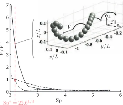
1 correspondstoaregimeatwhichbendingwavesareimmediatelydampedandthefreeendismotionless[19].

Theexperimentof[80]issimilarto[79] exceptfor thattheactuationatthebaseisrotational.Here,thefilament was rotatedatafrequency

ζ

formingabaseangle

α

0

=

0

.

262 rad withtherotationaxis.

Inbothcontributions,theresultingfiberdeformationsweremeasuredandcomparedtoResistiveForceTheoryforseveral valuesofSp.Simulationsofsuchexperiments[79,80]wereperformedwiththeGearsModel.

3.4.1. Numericalsetupandboundaryconditionsatthetetheredbaseelement

Corresponding kinematic boundary conditions for BM are prescribed with the constraint formulation of the Euler– Lagrangeformalism.

3.4.1.1.Planaractuation Inthecaseofplanar actuation[79],weconsiderthatthetethered,i.e. thefirst,beadisplacedat theoriginandhasnodegreeoffreedom

½

_r

_˙

c

1

=

0

,

ω

c

1

=

0

.

(59)

Denote

α

0 theangleformedbetweenex ande1,2.

Thetrajectoryofbead2 mustfollow

rc₂

(

t

) =





2a cos(

α

0sin(ζt

))

0 2a sin(

α

0sin(ζt

))





.

(60)

Thetranslationalvelocityofthesecondbeadr

˙

2

(

t

)

isthusconstrainedbytakingthederivativeof(60)

˙

rc₂

(

t

) =





−2a

α

0

ζ

cos(ζt

)

sin(

α

0sin(ζt

))

0

2a

α

0

ζ

cos(ζt

)

cos(

α

0sin(ζt

))



3.4.1.2. Helicalactuation Inthecaseofhelicalbeating[24,80],theanchorpointofthefilamentisslightlyoff-centeredwith respecttotherotationaxisex[24]:r

(

0

)

= δ

0(cf.Fig. 13,left inset).[24]measuredavalue

δ

0

=

2 mm withafilamentlength

varyingfrom L

=

2 cm to10 cm.Herewe take

δ

0

= ˜

δ

0sin

α

0 with

δ

˜

0

=

2

.

7a andvarythefilamentlength bychangingthe

numberofbeadsNbtomatchtheexperimentalrange

δ

0

/

L

=

0

.

1

→

0

.

02.Thepositionofbead1 mustthenfollow

rc₁

(

t

) =







˜

δ

0cos(

α

0sin(ζt

))

cos(

α

0cos(ζt

))

˜

δ

0cos(

α

0sin(ζt

))

sin(

α

0cos(ζt

))

˜

δ

0sin(

α

0sin(ζt

))







.

(62)

Thetranslationalvelocityofthefirstbeadr

˙

1

(

t

)

isthusconstrainedbytakingthederivativeof(62)

˙

rc₁

(

t

) =















˜

δ

0

α

0

ζ [−

cos(ζt

)

sin(

α

0sin(ζt

))

cos(

α

0cos(ζt

))

+

sin(ζt

)

sin(

α

0cos(ζt

))

cos(

α

0sin(ζt

))]

˜

δ

0

α

0

ζ [−

cos(ζt

)

sin(

α

0sin(ζt

))

sin(

α

0cos(ζt

))

−

sin(ζt

)

cos(

α

0cos(ζt

))

cos(

α

0sin(ζt

))]

˜

δ

0

α

0

ζ

cos(ζt

)

cos(

α

0sin(ζt

))















.

(63)

Andtherotationalvelocityissettozero

ω

1

=

0.

Thevelocityofthesecondbead

˙

rc₂

(

t

)

isprescribedinsynchronywithbead1:

˙

rc₂

(

t

) =















( ˜δ

0

+

2a)

α

0

ζ [−

cos(ζt

)

sin(

α

0sin(ζt

))

cos(

α

0cos(ζt

))

+

sin(ζt

)

sin(

α

0cos(ζt

))

cos(

α

0sin(ζt

))]

( ˜δ

0

+

2a)

α

0

ζ [−

cos(ζt

)

sin(

α

0sin(ζt

))

sin(

α

0cos(ζt

))

−

sin(ζt

)

cos(

α

0cos(ζt

))

cos(

α

0sin(ζt

))]

( ˜δ

0

+

2a)

α

0

ζ

cos(ζt

)

cos(

α

0sin(ζt

))















.

(64)

The rotationalvelocity

ω

2 isconsistentlyconstrained bythe no-slipcondition.The three-dimensionalcurvature

κ

is

dis-cretizedwith(34).

Inbothcases,imposingactuationatthebaseofthefilamentthereforerequirestheadditionofthreevectorialkinematic constraints,(59)and(61),totheno-slipconditions:Nc

=

3

(

Nb

−

1

)

+

3

×

3.TheadditionalJacobianmatrixJact writes

Jact

=





I3 03 03 03

· · ·

03 03 03 I3 03 03

· · ·

03 03 03 03 I3 03

· · ·

03 03





.

(65)

Thecorrespondingright-handsideBact containstheimposedvelocities

Bact

=





0 0

−˙

rc₂





(66)

forplanarbeating,and

Bact

=





−˙

rc₁ 0

−˙

rc₂





(67)

forhelicalbeating.

Jact and Bact are simply appended to

J

J

J

and B respectively; corresponding forces and torques

F

c are computed as

explainedbeforeinSection2.2.

3.4.2. Comparisonwithexperimentsandtheory

The dynamics of the system can be described by balancing elastic stresses (flexion andtension) with viscous drag. Subsequentcouplednon-linearequationscanbe linearizedwiththeapproximationofsmalldeflectionsorsolvedwithan adaptiveintegrationscheme[23,25,81].

3.4.2.1. Planaractuation [79] consideredbothlinearandnon-lineartheoriesandincludedtheeffectofasidewall byusing thecorrectedRFTcoefficientsof[82].

Simulations are in good agreement with experiments, linear and non-linear theories for Sp

=

1

.

73

,

2

.

2

,

and 3

.

11

(Fig. 12). Even though sidewall effects were neglected here, the Gears Model provides a good description ofnon-linear

Fig. 12. Comparisonwithexperimentsandnumericalresultsfrom[79].GearsModelresultsaresuperimposedontheoriginalFig. 3of[79].Snapshotsare shownforfourequallyspacedintervalsduringthecycleforonetailwithα0=0.435 rad. :experiment, :lineartheory, :non-lineartheory,—:

Gears Model, (a)ζ =0.5 rad s−1_{, Sp=1.73. (b)ζ =1.31 rad s}−1_{, Sp=2.2. (c)ζ =5.24 rad s}−1_{, Sp=3.11.}

Fig. 13. Comparisonwithexperimentsfrom[80].(Insets)EvolutionofthefilamentshapewithSp4_{.Snapshotsareshownfortwentyequallyspacedintervals}

duringoneperiodatsteadystate.Graylevelfadesastimeprogresses.Leftinset:δ0/L isthedistanceofthetetheredbeadtotherotationaxis,d/L isthe

distance of the free end to the rotation axis. (Main figure) Distance of the rod free end to the rotation axis normalized by the filament length d/L. E: experiment,":GearsModelwithnoanchoringdistanceδ0/L=0,2:GearsModelwithδ0/L=0.1→0.02 asin[24].

3.4.2.2. Helicalactuation Oncesteadystate was reached, [80] measuredthe distanceofthetip oftherotatedfilament to therotationaxisd

=

r

(

L

)

(cf.Fig. 13,left inset).Fig. 13comparestheir measures withournumericalresults.Insets show theevolutionofthefilamentshapewithSp.Theagreementisquitegood.Numericalsimulationsslightlyoverestimated for 30

<

Sp4

<

90.Thismaybe duetothelack ofinformationtoreproduce experimentalconditions and/orto measurement errors. As stated in [24], takingthe anchoring distance

δ

0 into account is important to match the low Sperm number