Current Account Balances, Exchange
Rates, and Fundamental Properties of
Walrasian CGE World Models: A
Pedagogical Exposition
BY ANDRÉ LEMELINa
This paper addresses theoretical aspects of global multinational trade models of the computable general equilibrium (CGE) type. We define and discuss the concepts of model homogeneity, model closure rules, and consistency in calibration. We examine and illustrate these issues using a highly simplified skeleton model derived from the PEP-w-1 CGE world model, to represent the essential structure of world trade models. Model closure issues, including how to correctly fix current account balances, are scrutinized. We also consider the role of nominal exchange rates in Walrasian “real” CGE models (without money), which can be, and often are written without exchange rates. But when exchange rates are present, we show that a model can be solved equivalently by exogenously fixing either exchange rates (FE) or regional price indexes (FP), and we weigh the advantages of either closure for economic interpretation of simulation results. The model is implemented in GAMS and is made available to readers as a supplementary download.
JEL codes: C68, D58, F47
Keywords: Computable general equilibrium models (CGE); Global trade models; CGE model closures; Current account balance; Exchange rate.
1. Introduction
There is an abundant literature on macro-economic closures for single country, open-economy models (Decaluwé et al., 1988; Delpiazzo, 2010 contains a recent comprehensive review; Dewatripont and Michel, 1987; Rattsø, 1982; Sen, 1963). In the present paper, however, we are not concerned with closures in single-economy models, but rather with issues that arise in the context of global multinational models, typically, trade models. In addition to model closures, we explore a few
a Urbanization and Culture Society, Institut National de la Recherche Scientifique (INRS-UCS), 385 rue Sherbrooke est, Montréal, QC, Canada H2X 1E3 (andre_lemelin@ucs.inrs.ca).
related issues that are rarely dealt with explicitly in CGE multinational modeling: model homogeneity, the role of exchange rates, calibration neutrality and consistency, and testing for calibration consistency and model homogeneity.
Indeed, there seems to be a void in the literature regarding these issues, each of which will be addressed in turn.
Closures: Global models, as opposed to single-country, open-economy models or multiregional non-global models, are “closed” systems, in that there is no “Rest of the world”. It follows that the worldwide sum of current account balances, when expressed in a common currency, must be zero. This rules out the unconstrained flexible current account closure sometimes used in non-global models. As a matter of fact, exogenous trade balances (which ensure the zero-sum constraint) are a common form of closure in global models, but the constraint is seldom explicitly stated or its form motivated.1 We also extend the formal
discussion of closures to systematically examine other possibilities, only to conclude that they are not feasible. This underlines the fact that selecting closure rules cannot be reduced to the simple counting of equations and variables.
Exchange rates: Another feature of global models is that the economic reality they represent involves multiple currencies. Data sources such as the GTAP database convert all monetary values to a common currency, and many global models are implemented without exchange rates, for example GTAP (Hertel 1997), or MIRAGE (Bchir et al., 2002a, 2002b; Decreux and Valin, 2007). In most Walrasian CGE world models that do have exchange rates, their nominal values are fixed (one exception is the Globe model: McDonald and Thierfelder, 2016). Here we propose endogenous nominal exchange rates, with fixed regional numéraires, as a model design which facilitates interpretation of results.
Calibration: Calibration procedures, including the implications of price × volume factoring, are generally not discussed.2 Here, the concepts of
homogeneity, closure and calibration neutrality and consistency are defined, and then related to practical issues of model specification, in a single integrated exposition. This third set of issues relates to any CGE model, not only global ones.
To examine and illustrate the issues we tackle, we develop a highly simplified skeleton model derived from the PEP-w-1 worldwide CGE model (Lemelin,
1 The topic of endogenous current account balances, often discussed under the heading of “international capital mobility”, is not addressed in this paper. Indeed, capital is internationally mobile and current account balances are endogenous in several global CGE dynamic models: the current version of GTAP and GTAP-Dyn (Ianchovichina and McDougall, 2001; Ianchovichina et al., 2000); the G-Cubed model (McKibbin and Stoeckel, 2009; McKibbin and Wilcoxen, 1999); the DART model (Hübler, 2011; Springer, 2003); the PEP-w-t-fin model (Lemelin, Robichaud, and Decaluwé, 2013, 2014).
2 McDonald and Thierfelder (2016, p.19) state their normalization rule explicitly, but do not discuss it.
Robichaud, Decaluwé & Maisonnave, 2013), but which represents the essential structure of several world trade models. It should be mentioned that our skeleton model has been elaborated using a SAM (Social Accounting Matrx)-based approach and has been implemented in GAMS. It follows that some technical points may not be relevant to other approaches (such as models implemented in GEMPACK), but the principles discussed are generally applicable to CGE modeling.
In Section 2, we present the basic concepts: model homogeneity, model closure, and calibration consistency. The theoretical model is presented in Section 3 (Model 1). In Section 4, the model is simplified, and redundant equations are identified and deleted (Model 2). Closure rules are first discussed in reference to Model 2 (Section 5). Next (Section 6), the role of exchange rates is clarified; the model is re-written in terms regional currencies, and nominal exchange rates are introduced (Model 3). Closure rules are revisited, detailing the choice between fixed exchange rates (FE) or fixed regional price (FP) closures; and calibration consistency is discussed. A brief conclusion wraps up the paper.
The implementation of Model 3 in GAMS is presented in Appendix K, and all of the GAMS programs and files are provided with this paper as supplementary online material. Readers are strongly encouraged to use the GAMS programs to test some of the ideas raised in the paper and thus gain a more hands-on understanding.
2. Concepts
2.1 Model homogeneity and Walras’ Law
Model homogeneity derives from microeconomic theory. The theory states that supply and demand functions derived from optimizing are homogenous of degree zero in prices and income (or more generally prices and nominal values). Formally, a CGE model is a set of simultaneous equations relating variables, some of which are endogenous (determined within the model), the rest being exogenous. The core of a CGE model consists of equations representing consumer and producer optimizing behavior, and market equilibrium. A CGE model solution is a Walrasian competitive general equilibrium: all optimizing economic agents meet their (first-order) optimality conditions, subject to their budget constraints, and all markets are in equilibrium. Without money, the set of equations which constitute the model is homogenous of degree zero in prices.
To formalize the definition of homogeneity and generalize it a little, let us distinguish the three types of variables a model may contain: volume variables, price variables, and nominal variables. Some nominal variables are the product of a volume and a price, but others cannot be factored into volume and price. They just represent payments made from one agent to another, such as transfers. With that distinction in mind, a model solution may be characterized as a triplet of
vectors
q,p,n
, containing volume (q), price (p), and nominal (n) variables. In a homogenous model, if
q,p,n
is a solution to the model, then
q,p,n
is also a solution, for any > 0. In other words, multiplying all prices and nominal values by a constant doesn’t disturb the equilibrium, because it leaves relative prices unchanged. This is the principal implication of homogeneity: only relative prices matter. Prices are determined only up to a factor of proportionality and their absolute level is indeterminate.The absolute level of prices is indeterminate because model homogeneity implies that one equation is redundant: there is one more price variable than the number of independent market equilibrium equations. This is generally referred to as Walras’ Law (Léon Walras, 1834-1910). Consider an economy where producers maximize their profits subject to their production function, and consumers own all factors of production, receive all factor income, and maximize their utility subject to their budget constraint.3 For every good (factor or
commodity), excess demand is defined as the sum of demands by all agents, minus the sum of supplies by all agents, for some price vector.Denote the vector of excess demands as
p . In equilibrium, demand equals supply, and
p* , where p* is the equilibrium price vector. Walras’ Law states that for any p (equilibrium or not), the total value of excess demands is zero: p
p . This isa straightforward consequence of respecting budget constraints: since p
p is the sum of all expenditures and incomes of all agents, if all budget constraints are satisfied, then that sum must be zero. A corollary of Walras’ Law is that, if all markets but one are in equilibrium for some price vector, then the remaining market must also be in equilibrium, because the value of excess demand on that market cannot be different from zero. It follows that in a model with N markets, there are only N–1 independent market equilibrium equations, and the Nth isredundant.
That leaves one degree of freedom, and the model is completed by exogenously fixing the price of one good, which plays the role of numéraire. The value assigned to the price of the numéraire determines the level of prices, and all other prices and nominal values in the model are expressed in terms of the price of the numéraire.4
3 This implies that all profits are distributed to consumers. Walras’ Law can be demonstrated in a less restrictive setting, but our objective here is to put forth the principle behind Walras’ Law, and so we keep its exposition as simple as possible.
4 Strictly speaking, the word numéraire designates the commodity relative to the price of which the prices of all other commodities are expressed. But for convenience, we take the shortcut of using the word “numéraire” to designate the price of the numéraire commodity. This allows us to say, for example, that all prices are expressed in terms of the numéraire
Homogeneity has two implications regarding the choice of a numéraire and of its value. First, although it may be convenient to set the numéraire at 1, the value assigned to the numéraire is arbitrary. That is quite obvious from the definition of homogeneity: if
q,p,n
is a solution to the model when the numéraire is set at 1, then
q,p,n
is also a solution, when the numéraire is set at any > 0. A second implication is that the choice of numéraire is arbitrary. Suppose that commodity i is chosen as the numéraire, with its price pi set atpi ; then changing the numéraire for commodity j and setting its price at pj is equivalent to changing from solution
q,p,n
to
q,p,n
with pj pj , where pj is the value of price j when the numéraire is commodity i.In other words, if a model is truly homogenous, the solution values of real (volume) variables and all price and nominal value ratios are supposed to be: independent of which commodity is taken as the numéraire; independent of which region is taken as the reference region when the numéraire is a regional commodity (a particular case of the preceding); and independent of the particular value given the price of the numéraire, whatever commodity plays that role.
Of course, not all CGE models are “purely” Walrasian. But most non-monetary CGE models nevertheless retain the property of model homogeneity. In any case, if a model is not homogeneous, it should be by purpose, not by accident or by mistake. So it is useful to check for model homogeneity.
It is easy enough to check simple models for homogeneity, but it may be tricky with complex models. With simple models, one can check for homogeneity analytically, by examining the equations. Homogeneity can also be verified numerically, by transforming a
q,p,n
simulation solution into a
q,p,n
solution, and then verifying whether the model equations are satisfied. Another approach, somewhat more demanding, is to compare simulation solutions obtained with different values of the numéraire or with different numéraires and verify that the alternate solutions
q,p,n
and
q,p,n
satisfy the relationship
q,p,n
=
q,p,n
for some > 0.The latter approach is more demanding, because it requires that the model equations be written in such a way as to adjust to an arbitrary value of an arbitrary choice of numéraire (this is illustrated in the homogeneity tests outlined in Section 6.3).5 Moreover, the model closure must be formulated with care to avoid the many
– much more concise and comprehensible than the first sentence of this footnote! In addition, it should be mentioned that in some models, prices are expressed relative to some global price index, in which case the numeraire good is an aggregate.
5 I understand that in GEMPACK, model homogeneity is automatically checked by shocking the numéraire.
pitfalls of inadvertantly de-homogenizing the model. Regarding our skeleton model, we shall see, in particular, that, under fixed exogenous current account balance closures, the way current account balances are fixed is critical (Section 4.2). 2.2 Model closure
With a CGE model, as with any system of simultaneous equations, the number of independent equations must be equal to the number of endogenous variables for the model to have a solution (the model must be square).6 If there are more
equations than variables, the model is overdetermined; if there are fewer equations than variables, the model is underdetermined. The issue of model closure concerns the theoretical foundations and meaning of the choices made by the modeler to make the number of equations and the number of variables equal.
In a way, taking into account Walras’ Law to discard a redundant equation, and defining a numéraire to make the model square, can be viewed as one aspect of model closure. But the issue of model closure is broader and more substantive.
The discussion of macroclosures in single-economy models was initiated by Sen (1963) in relation to the debate on income distribution. Essentially, Sen showed that competing views of the economy could be characterized by the choice of which equation to eliminate in an overdetermined model (this is nicely summarized in Rattsø, 1983). In contrast, contemporary CGE models are usually underdetermined, left open to different views of the economy. It is up to the model user to choose which equation or constraint to add to the model in order to “close” it and to make it “square”, with as many equations as there are variables.7
Here we are concerned with multinational (or multiregional) world models, and we will examine model closures that take the simple form of fixing one or more variables exogenously. Specifically, we consider:
1) How many variables must be exogenously fixed?
2) Which variables can be sensibly designated as exogenous to close the model?
3) Does the choice of exogenous variables always matter? Can the same model closure be implemented by fixing alternative sets of variables? Put otherwise, are there model closures which are different in their implementation, but are mathematically and economically equivalent? Underlying question 1 is the matter of redundant equations. The number of variables to fix exogenously is equal to the number of degrees of freedom in the model, given by the difference between the number of endogenous variables and the number of independent equations. To accurately count the number of
6 It would be tempting to add “unique”. But the possibility of multiple solutions cannot always be ruled out in models that are constrained nonlinear systems (CNS).
independent equations, one must be able to identify redundant equations in the model. This is of practical importance when the model is submitted to a GAMS solver as a CNS (constrained nonlinear system) class model, because GAMS will reject the model as not square if it contains redundant equations, even if, mathematically, redundant equations do no harm.
2.3 Calibration neutrality and consistency
To implement a CGE model, values must be assigned to its parameters and benchmark variables. This process is called model parametrization and the usual practice in CGE modeling is to proceed in two steps: (1) assign values to a set of so-called “free” parameters, and (2) calibrate the model. The distinction between free and calibrated parameters is somewhat arbitrary, but it is customary to treat elasticities in behavioral functions as free parameters, for which modelers use econometric estimates, or else borrow estimates from the literature. Model calibration on the other hand is the process of assigning values to parameters and benchmark variables, given the values of free parameters, from the information contained in the underlying data base (often organized in the form of a social accounting matrix SAM), combined with the restrictions imposed by the theoretical specification of the model (model equations).
Price × volume factoring: Variable benchmark values in particular are routinely calibrated from SAMs. SAM entries are transaction flows. Part of the calibration procedure consists in a factoring of SAM transaction flows into price × volume products. But SAM transaction flows generally represent composite aggregates for which there is no clear physical unit of measurement. Even when the volume can be measured unambiguously, factoring depends on the choice of unit of measurement, which is arbitrary: 454 grams of something at 1¢ a gram is the same as one pound at $4.54 per pound. It follows that the price × volume factoring is arbitrary, constrained only by the value of their product. However, although the factoring of SAM transaction flows is arbitrary, there are consistency requirements to satisfy: we return to these shortly.
But first, let us briefly recall an implication of the arbitrariness of price × volume factoring that is occasionally neglected in the interpretation of CGE simulation results, namely that prices and volumes must be viewed as indices: price or volume levels are meaningless; only proportional changes are meaningful.8 When, in a
simulation solution, a transaction flow increases or decreases relative to its benchmark value, the CGE model provides a decomposition of the change into price
8 Of course, if complementary information makes it possible to convert SAM flows into proper quantities, then the volume indices can be translated to quantities. For example, the volume of full-time equivalent employment, when it is known, provides a metric to convert the SAM flow of labor income into the corresponding number of jobs.
variation and volume variation. This is exactly the kind of decomposition that is needed to correctly interpret, say, an increase in consumption expenditures when the consumer price index changes.
Neutrality of the identification constraints: Once the so-called “free” parameters (elasticities and the like) have been specified, the number of unknowns (parameters and benchmark variables) usually remains greater than the number of constraints (SAM values and model equations). Therefore, to solve the calibration problem, it is necessary to impose additional constraints, which we shall call “identification constraints”. Identification constraints often consist in fixing the level of a set of variables which are defined only up to a factor of proportionality (like in price × volume factoring). There is in general no unique set of identification constraints that will complete the calibration procedure, but such constraints, given that they are based neither on observation (SAM flows), nor on theory (model equations), should be non-restrictive, or “neutral”. By that, we mean that they should not affect model results. Formally, we define neutrality as follows. Given a consistent calibration procedure, a set of identification constraints is said to be neutral if it results in a model for which the relative variation of a variable between any simulation solution and its benchmark is the same as with any other set of neutral identification constraints.9
A concrete example of neutrality is given in subsection 6.2 with respect to the arbitrariness of price × volume factoring. We show that the volume of a constant elasticity of substitution (CES) or constant elasticity of transformation (CET) aggregate may be benchmarked as the sum of its components without implicitly imposing perfect substitutability, or alternatively, that the price of the aggregate may be arbitrarily set at 1 without imposing price equality.
Consistency of the calibration procedure: The calibration procedure solves what has in effect become a simultaneous equations problem, as defined by the values of free parameters, the model data base (SAM), the model specification (equations), and the identification constraints. But rather than being shifted to a solver program, the calibration problem is generally solved through a sequence of statements assigning values to the unknown parameters and benchmark variables. This is equivalent to solving the system of equations after having triangularized
9 There is the appearance of a circular problem here. The model cannot be solved if it is not calibrated, and it cannot be calibrated without some set of identification constraints. So checking numerically whether simulation results are the same with or without a given set of identification constraints actually means comparing simulation results obtained using two different sets of identification constraints. Unless one of the two has been demonstrated to be neutral, the comparison is not logically conclusive. However, in this modeler’s experience, there usually exists a set of identification constraints that can be shown mathematically to be neutral.
the problem. So the art of calibration is very much the art of correctly sequencing the assignments.
What then is “calibration consistency”? Formally, calibration consistency could be defined as the requirement that the calibration procedure be truly equivalent to solving the (correctly) triangularized calibration problem. Practically speaking, calibration inconsistency may result from errors in the sequencing of assignments or in formulations that fail to preserve the neutrality of some identification constraint.
Test of neutrality and consistency: Two models are equivalent if the relative variation of all variables between any simulation solution and the benchmark is the same in both. To test a calibration procedure against another is to determine whether the models that result from the two procedures are equivalent or not. Mathematically, let PiC,k,S be the value of price variable i, in solution k of the model calibrated using a calibration procedure C and a set S of identification constraints; subscript k is equal to 0 for the benchmark, and to 1 for the simulation. Also let
S C
k j
Q ,, be the value of volume variable j in solution k of the model calibrated using C and S. Sets S may differ in the choice of variables or in the values assigned or both. Then the resulting models are equivalent if
S C h S C h S C i S C i S C h S C h S C i S C i P P P P P P P P , , , , , , , , , , , , , , , , (1) S Cj S Cj S Cj S C j Q Q Q Q ,, ,, , , , , (2)
for any pair C1, C2 of calibration procedures, and pair S1, S2 of sets of identification calibration constraints. The first condition states that variations in the price of any good i relative to any other h must be the same in both cases; the second condition says that proportional volume variations must be equal.
If these two conditions are not realized, it may be for one of two reasons. First, one of the pair of sets of constraints S1 and S2, or both, may be restrictive (non-neutral). In that case, the problem is with the identification constraints, not with the calibration procedure. And either the identification constraints must be replaced with a set of neutral constraints, or the model specification should be extended to include one or more of these non-neutral constraints. As an example of the latter situation, the assignment of values to elasticity parameters is not neutral; for that reason, elasticities are treated as “free” parameters, not as identification constraints, and they are part of the model specification.
The second reason for which conditions (1) and (2) may be violated is that the calibration procedure is not consistent. In particular, the way in which the
constraints are implemented may be inconsistent in the sense that the calibration procedure is compatible only with one particular set of identification constraints. An example is given in subsection 6.3.3, where a calibration shortcut which sets a given price at 1 is valid only if other previously determined prices are also set at 1, while their value should be arbitrary.
To summarize, model parameters and benchmark values cannot be calibrated from SAM values and model equations alone, even after assigning values to the free parameters: the solution of the calibration problem remains undetermined without additional “identifying” constraints. However, these identifying constraints are not totally arbitrary: they must be neutral and applied consistently. Moreover, the calibration procedure must be a correct implementation of the solution to the triangularized calibration problem.
3. Skeleton model: Model 1
We now define the theoretical model which will serve as our departure point to explore the issues raised in the introduction.
3.1 Model description
There are N regions. There is a single regional agent in each region, and there are no taxes. All prices and nominal values are expressed in terms of the international currency.
There is a single good, and production factors are fixed. With full employment, this implies that output is fixed in each region z, and that the regional agent’s income is equal to the value of production.
The model is static, so we can define “consumption” to include both current consumption and investment. It follows that domestic savings, the difference between income and “consumption” (which includes savings), are equal to the current account balance (CAB).10
The model retains the Armington hypothesis regarding the distribution of demand between imports and the domestically produced good, and for imports, between source regions, using CES aggregator functions. Similarly, production is allocated between domestic sales and exports, and for exports, between regions of destination, according to CET functions.
This model is close to a Walrasian pure exchange economy. It is illustrated in Figure 1 for the case of two regions. But in what follows, we deal with an N-region model.
10 In other words, in this skeleton model, the definition of domestic savings is much narrower than normally: here, it is the surplus of income over domestic absorption, whereas it is normally the surplus of income over current private and public consumption.
Figure 1. Skeleton model of international trade
Region 1
Region 2
Domestic demand Demand for international imports Demand for domestic goods CE S Armi ng tonDomestic savings = CAB (> or < 0) CAB of Region 1 = – CAB of Region 2 Domestic production Supply of international exports CE T Supply to the domestic market Value of production = regional income Supply of international exports Supply to the domestic market Domestic production Value of production = regional income Demand for domestic goods Demand for international imports
Domestic savings = CAB (> or < 0) CE T Domestic demand CE S Armi ng ton
At the top of Figure 1, domestic production is sold on the domestic market or exported, following a CET function. The value of domestic production constitutes the regional agent’s income, which is divided between domestic demand, and domestic savings (which may be negative). Domestic demand is distributed following a CES function between domestic production and imports. The imperfect-substitutability Armington hypothesis is what makes it possible to have both imports and exports even if there is a single good. Each region’s current account balance (CAB) is given by the value of exports, minus the value of imports. Given that investment is subsumed in consumption, the CAB is equal to domestic savings. Also, in the particular case of two regions, one region’s CAB is equal to minus the other’s.
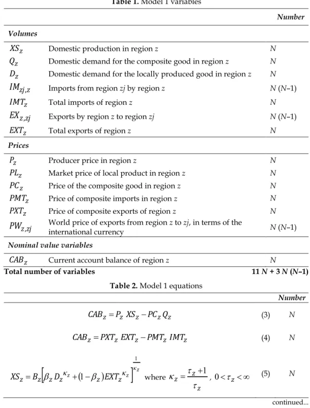
Table 1 lists the Model 1 variables, and Table 2 lists the equations (for a more detailed presentation, see Appendix A, supplemental online material). The regions are designated by subscripts z,zj,zjj
,,N
(a different style of subscripting might use i, j, and k, rather than z, zj, and zjj). For instance, in variables IMzj,z,zj z
EX , , and PWz,zj, the first subscript designates the region of origin, and the
second the region of destination of goods in trade flows. This physical flow from-to convention for subscript order is applied throughout the model. Also note that
z z
IM , , EXz,z , and PWz,z is undefined, which reflects the fact that there is
no international trade between a country and itself.12
Model 1 being a very simple model, it is easy to verify its homogeneity analytically. Indeed, for any set of variable values that solves equations (3)-(18), a new set of variable values obtained by multiplying all prices and nominal values by some positive constant is also a solution. Homogeneity implies that in the model, prices (and nominal values) are defined only up to a factor of proportionality, so that the modeler must choose a numéraire and set its level.
The number of variables in the model is 11 N + 3 N (N – 1), where N is the number of regions. The number of equations in Table 2 is 12 N + 1 + 3 N (N – 1) equations. The model appears to be overdetermined. But, as we shall see, it is not.
12 In a real global model, the world is divided into regions, some of which include more than one country: then, international trade within a multi-country region is possible.
Table 1. Model 1 variables
Number Volumes
z
XS Domestic production in region z N
z
Q Domestic demand for the composite good in region z N
z
D Domestic demand for the locally produced good in region z N z
zj
IM
, Imports from region zj by region z N (N–1)z
IMT Total imports of region z N
zj z
EX
, Exports by region z to region zj N (N–1)z
EXT Total exports of region z N
Prices
z
P Producer price in region z N
z
PL Market price of local product in region z N
z
PC Price of the composite good in region z N
z
PMT Price of composite imports in region z N
z
PXT Price of composite exports of region z N
zj z
PW
, World price of exports from region z to zj, in terms of theinternational currency N (N–1)
Nominal value variables
z
CAB Current account balance of region z N
Total number of variables 11 N + 3 N (N–1)
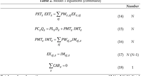
Table 2. Model 1 equations
Number z z z z z P XS PC Q CAB (3) N z z z z z PXT EXT PMT IMT CAB (4) N
z z z z z z z z z B D EXT XS
where z z z
, z (5) N continued...Table 2. Model 1 equations (continued) Number z z z z z z z PL PXT D EXT (6) N
X z X z zj zzj X zj z X z z B EX EXT
, , where X z X z X z , zX (7) N
X z X z z X zj z zj z X z z zj z PXT PW B EXT EX , , , (8) N (N–1)
z z z z z z z z z A D IMT Q
where z z z
,z (9) N z z z z z z z PMT PL D IMT (10) N M z M z zj zjz M z zj M z z A IM IMT
, , where M z M z M z , zM (11) N
M z M z z zj z z M z zj M z z z zj PW e PMT A IMT IM , , , (12) N (N–1) z z z z z zXS PL D PXT EXT P (13) N continued...Table 2. Model 1 equations (continued) Number
zj zzj zzj z zEXT PW EX PXT , , (14) N z z z z z zQ PL D PMT IMT PC (15) N
zj zjz zjz z z IMT PW IM PMT , , (16) N z zj z zj IM EX , , (17) N (N–1)
z z CAB (18) 1Total number of equations 12 N + 3 N (N–1) + 1
4. Redundant equations and reduction of the model: Model 2
How many variables and equations are there in the model? If the number of independent equations is greater than the number of variables, then the model is over-determined and infeasible. On the other hand, if the number of independent equations is less than the number of variables, then some variables have to be made exogenous and fixed in the closure. So it is necessary to identify and eliminate redundant equations from the model.
From Tables 1 and 2, Model 1 appears to have 11 N + 3 N (N – 1) variables: 11 (groups of) variables indexed in z, and 3 (groups of) variables indexed in z,zj. The equation count is 12 N + 3 N (N – 1) + 1: 12 (groups of) equations indexed in z, 3 (groups of) equations indexed in z,zj, plus the single equation (18). So the model appears to have N + 1 equations too many. However, as we demonstrate in Appendix B (supplemental online material), several equations are redundant: equations (7) and (8) together imply (14), which is therefore redundant; equations (11) and (12) together imply (16), which is therefore redundant; equations (4) and (17) together imply (18), which is therefore redundant; equations (13), (15) and (3) together imply (4), which is therefore redundant.
In addition, it is shown in Appendix B that Walras’ Law can take the following form in our model: if equation (3) is satisfied for N – 1 regions, then it is also satisfied for the Nth one. Therefore, one equation of the set (3) may be discarded
as redundant. So we can arbitrarily pick some region zleon, zleon
,,N
(zleon is a mnemonic for Léon Walras), and remove equation (3) for that single region. Note that with the removal of the equation relating to zleon, the variable CABzleonno longer appears in the model, but its value may be computed using the suppressed equation.
Some modelers sidestep the task of seeking out and eliminating redundant equations by changing the constrained nonlinear system (CNS) into a nonlinear programming (NLP) problem with a dummy objective variable set equal to a constant. This is risky, because the solver will find a solution even if the model misses a closure equation, which usually implies that the solution produced by the solver depends on the initial values of the variables, because when a closure equation is missing, the solution is generally not unique. This point is illustrated with the help of a simple example in Appendix C (supplemental online material). We now rewrite the model, discarding redundant equations. After eliminating equations (4), (14), (16) (18), and one equation of the set (3), we are left with Model 2. The equations in Model 2, listed in Table 3, number 9 N – 1 + 3 N (N – 1), where N is the number of regions. The list of variables is the same as for Model 1, except that CABzleon no longer appears in the model; it is determined implicitly. Since it
no longer appears in the model, CABzleon is not to be counted as a model variable,
even if it appears in Table 3. So the reformulated model has 11 N – 1 + 3 N (N – 1) variables. Thus, Model 2 is underdetermined, it is 2N equations short. So the overdetermined appearance of Model 1 is nothing more than an illusion caused by the presence of redundant equations. Consequently, the closure of Model 2 will require adding 2N constraints, including fixing the numéraire. We also note that the homogeneity of Model 2 can be confirmed by examining it analytically in the same way as that of Model 1.
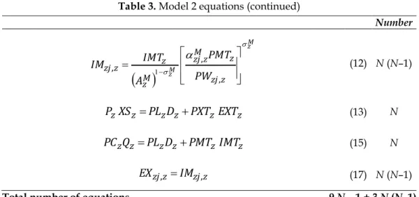
Table 3. Model 2 equations Number z z z z z P XS PC Q
CAB , for all zzleon (3) N–1
z z z z z z z z z B D EXT XS
where z z z
, z (5) N z z z z z z z PL PXT D EXT (6) N
X z X z zj zzj X zj z X z z B EX EXT
, , where X z X z X z , zX (7) N
X z X z z X zj z zj z X z z zj z PXT PW B EXT EX , , , (8) N (N–1)
z z z z z z z z z A D IMT Q
where z z z
i z (9) N z z z z z z z PMT PL D IMT (10) N M z M z zj zjz M z zj M z z A IM IMT
, , where M z M z M z , zM (11) N continued...Table 3. Model 2 equations (continued) Number
M z M z z zj z M z zj M z z z zj PW PMT A IMT IM , , , (12) N (N–1) z z z z z zXS PL D PXT EXT P (13) N z z z z z zQ PL D PMT IMT PC (15) N z zj z zj IM EX , , (17) N (N–1)Total number of equations 9 N – 1 + 3 N (N–1)
5. Closure of Model 2
Reviewing the list of variables in Table 1, it might appear that there are several candidates for being fixed in the closure rule. Here we shall go through the list critically, discarding possibilities that are incorrect in the general equilibrium framework. Throughout the review process, we maintain the neoclassical full-employment hypothesis, which is itself a closure rule, so that we restrict our attention to neoclassical closures.13 With production factors in fixed supply, in our
simple model, the neoclassical full-employment hypothesis implies that production is fixed: XSz XSz.
This adds N constraints to the model, leaving N degrees of freedom. 5..1 Neoclassical closure with fixed current account balances
In this section, we see how fixing CAB makes the model non-homogenous, and z
how homogeneity can be preserved by fixing a pseudo-volume variable CABX , z
the definition of which is not unique, however. Finally, we examine the substantive implications of fixing CAB beyond the issue of homogeneity. z
We begin with a closure rule that is very common in trade models14, which
consists in fixing current account balances for zzleon, in addition to fixing the
13 It would have been possible to consider non-neoclassical closures, such as fixing Q
z.
However, our goal is to illustrate the mathematical logic underlying the selection of closure rules, and restricting our attention to neoclassical closures makes the exposition more compact.
14 Recall however that there are several models with endogenous current account balances, as mentioned in a footnote in the Introduction.
numéraire. This adds (N – 1) + 1 = N constraints to the model, making it square. However, fixing CAB makes the model non-homogenous. The reason is that z
z
CAB is a nominal variable, and if CAB is fixed, the constraint it represents in real z
terms depends on the choice of numéraire and its value.
Formally, fixing CAB , z zzleon, means fixing N – 1 elements of the vector of nominal variables (n) in the
q,p,n
triplet which represents a model solution (see section 2.1). Now, homogeneity requires that if two simulations starting from the same set of benchmark values
q,p,n
, with different numéraires, yield solutions
q,p,n
and
q,p,n
respectively, then the solutions must satisfy the relationship
q,p,n
=
q,p,n
for some > 0. If N – 1 elements of the vector of nominal variables (n) are fixed, the relationship can hold only for = 1.Therefore, in a closure that preserves model homogeneity, current account balances must be fixed in real terms. One way to do this is to fix
z z PWINDEXCABX
CAB (19)
where CABX is fixed in the closure, and z
z zj zzj O zj z z zj zzj zzj z zj O zj z O zj z z zj O zj z zj z EX PW EX PW EX PW EX PW PWINDEX , , , , , , , , (20)is a Fisher index of bilateral trade prices, and superscript O designates benchmark values (equivalently, one could substitute IMz,zj for EXz,zj and IMOz,zj for EXOz,zj
in (20)).
By inverting (19) to obtain
PWINDEX CAB
CABXz z (21)
it is manifest that CABX is a pseudo-volume variable. The introduction of z CABX z
and equation (21) adds N + 1 variables, because it re-introduces CABzleon into the
model, and N equations. The introduction of PWINDEX adds one variable and one equation to the model. So the expanded model now has N + 1 additional equations, for a total of 10 N + 3 N (N – 1) equations, and N + 2 additional variables, for a total of 12 N + 1 +3 N (N – 1) variables, leaving 2 N + 1 degrees of freedom. With XSz
and CABX fixed (2 N variables), there is a single degree of freedom left. It is used z
to set the numéraire.
The user may pick any one price from one of the sets Pz, PLz, PCz, PMT , z PXTz
yield solutions where the volume variables are equal, and prices and nominal value variables are all proportional (relative prices are the same).
There are of course other ways to define CABX . Among the alternatives is the z
possibility of using another trade-price index, such as a Laspeyres index of bilateral trade prices, or of regions’ aggregate import prices, or of regions’ aggregate export prices; Paasche or any other type of price indexes could also be used. One could even define the “real” current account balance on the basis of a price that is not directly related to trade, such as, for example, the producer price in some particular region selected as a “reference region”. Let the reference region be designated by the index zr, zr
,,N
(the index used for the reference region is zr, to indicate that the reference region may be different from region zleon which is excluded from equation (3) under Walras’ Law). Then CABX can be defined as zzr z
z CAB P
CABX (22)
where Pzr is the producer price in the reference region.
It must be kept in mind, however, that the denominator that defines CABX z
must be the same for all regions z. It would be an error, for example, to define
z z
z CAB P
CABX , where the denominator is specific to each region. In that case, the implicit solution value of CABXzleon will be different from its fixed closure
value. Since CABXzleon does not appear in the model, GAMS will find a solution.
But the equation left implicit on account of Walras’ Law will be violated, as well as one or more of the redundant equations (4), (14), (16), and (18).
No matter how CABX is defined, provided that definition is admissible, the z
choice of the numéraire and its value is arbitrary. However, the way CABX is z
defined does matter! That is because different variants of CABX , when they are z fixed in the closure, impose different constraints in real terms. Indeed, CABX is a z
pseudo-volume variable, which does not have a clear-cut, unique definition. Although choosing a particular variant of CABX is not equivalent to choosing any z other, none of the possible specifications of CABX stands out as the natural one.z 15
It might be tempting to sidestep the issue of defining CABX while maintaining z
model homogeneity with respect to changes in the value of the numéraire by fixing
z
z CABX
CAB (23)
15 This issue does not arise in models such as GTAP where the current account balance is endogenous, although the definition of CABXz does matter for interpretation.
where is the numéraire; the value of CABX fixed in the closure is usually z CABOz
.16 Indeed, with this definition, the value of CAB automatically adjusts to any z
change in the value of the numéraire. Note that this approach is equivalent to defining CABX as z
z z CAB
CABX (24)
and fixing it in the closure. This shows that the approach in (23) implicitly defines
z
CABX in terms of the numéraire, so that changing the commodity that serves as the numéraire good modifies the closure in real terms. In other words, the model is homogenous with respect to changes in the value of the numéraire, but not with respect to changes in the choice of the numéraire good.
The following example illustrates this point. The model was run three times in GAMS17; in each run, the model is parametrized, the benchmark solution is
computed, and a simulation is performed (in this case, an increase in Region 3’s resources/output). All three runs use a fixed nominal CAB closure. In the first, z the numéraire is PWINDEX and it is fixed at 1. This, as we have seen, yields identical results to a fixed CABX closure with the same numéraire. In the second z
run, the value assigned to the numéraire PWINDEX is set at 2, and the value of fixed nominal CAB is doubled accordingly. In the third run, Region 3 is z
designated as the reference region, and the numéraire is changed to Pzr. Table 4. SAM and calibrated values
(numéraire PWINDEX) Social accounting matrix (benchmark)
Reg1 Reg2 Reg3 Tot
Reg1 100 10 110
Reg2 15 50 10 75
Reg3 5 30 35
CAB -10 15 -5
Tot 110 75 35 220
Benchmark Volumes Benchmark Prices
16 This strategy is applied in the Globe model (McDonald and Thierfelder, 2016), and it is used by van der Mensbrugghe (2010, see p.28-29).
17 The GAMS program which was actually used was not Model 2, but Model 3 with the FE closure and exchange rates set at 1 (see 6.2.1), which yields solutions numerically identical to Model 2’s.
Reg1 Reg2 Reg3 Reg1 Reg2 Reg3 DD 100 50 30 PL 1 1 1 EXT 10 25 5 P 1 1 1 IMT 20 10 10 PC 1 1 1 XS 110 75 35 PMT 1 1 1 Q 120 60 40 PXT 1 1 1
Bilateral trade volumes - Benchmark Bilateral trade prices - Benchmark
Reg1 Reg2 Reg3 Reg1 Reg2 Reg3
Reg1 10 Reg1 1
Reg2 15 10 Reg2 1 1
Reg3 5 Reg3 1
Source: Author calculations.
With PWINDEX, all benchmark volumes are the same as with PWINDEX
, and all prices are doubles. When the numéraire is Pzr, with Region 3 as the reference region, all benchmark values are the same as with PWINDEX. Now let us compare the simulation-to-benchmark ratios (Table 5).
Table 5. Simulation/benchmark ratios using different numéraires
PWINDEX = 1 PWINDEX = 2 Ref. region = 3,
zr
P
Reg1 Reg2 Reg3 Reg1 Reg2 Reg3 Reg1 Reg2 Reg3 Volumes DD 0.997 1.002 1.576 0.997 1.002 1.576 0.990 1.026 1.571 EXT 1.032 0.995 1.543 1.032 0.995 1.543 1.093 0.947 1.575 IMT 1.061 1.032 1.118 1.061 1.032 1.118 1.038 1.093 1.058 XS 1.000 1.000 1.571 1.000 1.000 1.571 1.000 1.000 1.571 Q 1.007 1.007 1.454 1.007 1.007 1.454 0.998 1.037 1.433
Bilateral trade volumes
Reg1 1.032 1.032 1.093 Reg2 0.912 1.118 0.912 1.118 0.872 1.058 Reg3 1.543 1.543 1.575 Prices PL 0.993 1.025 0.886 0.993 1.025 0.886 1.138 1.234 1.000 P 0.995 1.024 0.885 0.995 1.024 0.885 1.143 1.218 1.000 PC 0.988 1.023 0.922 0.988 1.023 0.922 1.133 1.227 1.047 PMT 0.962 1.010 1.052 0.962 1.010 1.052 1.111 1.195 1.218 PXT 1.010 1.022 0.876 1.010 1.022 0.876 1.195 1.185 1.001
Bilateral trade prices
Reg1 1.010 1.010 1.195
Reg2 1.000 1.052 1.000 1.052 1.161 1.218
Reg3 0.876 0.876 1.001
Source: Author calculations.
As expected, the nominal CABz closure is homogenous with respect to changes
in the value given to the numéraire, provided the exogenous value of CABz is properly adjusted: model results are equivalent, whether
PWINDEX
or
PWINDEX
(left and center panels of Table 5). However, the nominal CABz closure is not homogenous with respect to a change in the numéraire good: when the numéraire is changed fromPWINDEX
to Pzr , the simulation results are different, even if all benchmark values are the same as in the first run (right-hand side panel of Table 5).5.2 Neoclassical closure with a set of fixed volume variables
In this section we extend the formal discussion of closures to systematically examine other possibilities, only to conclude that they are not feasible. Specifically, if XSz is fixed, it is infeasible to fix another set of volume variables. We shall try
to understand why, and highlight the fact that selecting closure rules cannot be reduced to counting equations and variables.
Model 2 has 6 sets of volume variables in addition to XSz (See Table 1: Model
1 and Model 2 have the same sets of variables). Fixing
XS
z
XS
z is the form that the neoclassical full-employment hypothesis takes in the skeleton model. We now assert that, in this model, if XSz is fixed, it is infeasible to fix another set of volumevariables. This can be illustrated in a 2-region version of Model 2; the two-region version of Model 2 is detailed in Appendix H. It consists of equations (3) (for
zleon
z
), (5), (6), (9), (10), (13), (15) and (21)18, together with a trade-price indexre-defined for the two-region case
z z O z z z z z O z O z z O z z IMT PMT IMT PMT IMT PMT IMT PMT PWINDEX (25)and the two-region equilibrium conditions z zj
IMT
EXT
(26) * * z zj PMT PXT (27)From the 2-region version of Model 2, consider the sub-model consisting of equations (5),(9), and (26). Let us call this sub-model the Q-Model (Q for quantity). With two regions, there are 6 equations and 10 variables in the Q-model: XSz, Dz
, EXTz, Qz, IMTz. In principle, it should be possible to fix 4 of them, among which
z
XS . Figure 2 summarizes the two-region Q-model. The position of the CET
production frontiers in the north-west and south-east quadrants is determined by the fixed XSz. As long as the Qz are not fixed, the CES indifference curves in the
north-east and south-west quadrants are free to move inward or outward. Setting a pair of Dz, EXTz, or IMTz specifies a point on each of the CET frontiers defined
by XSz. Drawing perpendicular lines from these two points traces a rectangle. The
18 Equation (3) is the CAB definition; (5) is the CET transformation between domestic sales and exports, and (6) is the relative supply function; (9) is the CES aggregator between the domestic good and imports, and (10) is the relative demand function; (13) equates the value of production to the sum of the value of sales on the domestic market and exports; (15) equates total expenditures to the sum of purchases on the domestic market and the value of imports; (19) is the definition of CABXz.
solution corresponds to the values of Qz that make the indifference curve pass through the north-east and south-west corners of the rectangle.
Figure 2. The two-region Q-Model
It is quite obvious that if, a contrario, the Qz are fixed rather than the Dz, EXTz , or IMTz, there is no guarantee that a solution rectangle exists. Therefore, given
z
XS , Qz cannot be fixed arbitrarily.19 And if a solution exists, it may well not be
unique. Let us examine this more closely with the two-region Q-Model. Suppose the Qz are fixed:
Q
z
Q
z. Then combining equations (5), (9) and (26) yields
19 This kind of limitation is common in CGE models. Indeed, it was the central issue in Sen (1963).
z z z z z z zj z z z z z z z z z z z IMT B XS A Q IMT (28)(see Appendix I, supplemental online material). Given XSz and
Q
z, the pair ofequations (28) can be solved for IMTz; then EXTz and Dz follow from (26) and
either (9) or (5). The pair of equations (28) (IMT as a function of IMT, and IMT as a function of IMT) are plotted for different values of
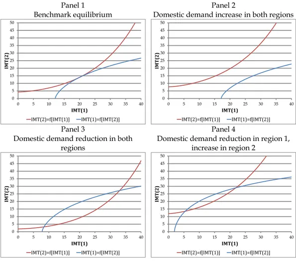
Q
z in the four parts of Figure 3.The two functions are convex: as a function of the other region’s imports, the imports of each region increase at a decreasing rate. The solution, of course, is given by the intersection of the two curves. In the benchmark equilibrium, the curves are tangent at the solution (Figure 3(a)). If the exogenous volume of domestic demand Q is increased in both regions (Figure 3(b)), the curves no z longer intersect: there is no solution. If, on the contrary, Q is reduced in both z regions (Figure 3(c)), then the solution exists, but it is not unique. Finally, Figure 3(d) illustrates a situation where Q is increased in one region, but reduced in the z other; in that particular case, there is a solution, but it is not unique.
This explains why, if one tries to close the model by fixing Q , then the z CONOPT solver cannot find a solution and issues the diagnostic “Pivot too small”, which “means that the set of constraints is linearly dependent in the current point and there is no unique search direction for Newton’s method so CONOPT terminates”.20
20 The reader can find this quote through the GAMS Help menu, under “Solver manual”. Click on CONOPT and navigate to Appendix A/Miscellaneous Topics/Constrained Nonlinear Systems or Square Systems Of Equations. The author of the CONOPT solver manual is Arne Drud, ARKI Consulting and Development A/S, Bagsvaerd, Denmark (http://www.conopt.com).
Panel 1
Benchmark equilibrium
Panel 3
Domestic demand reduction in both regions
Panel 2
Domestic demand increase in both regions
Panel 4
Domestic demand reduction in region 1, increase in region 2
Figure 3. Existence of a solution in the two-region Q-Model
What about closures that would fix D , z EXT , or z IMT , in addition to z XS ? z
We have shown above that such a closure determines all volume variables in the model, using equations (5), (9), and (26). The issue is then whether there exists a set of prices that can make those quantities equilibrium quantities. Given the calibrated values of the model parameters, there is no guarantee that there is such a set of prices. Moreover, if such a set of prices exists, the price equation sub-system becomes degenerate.
To illustrate this, consider once again the two-region model described in Appendix H. After removing the Q-model equations, the rest of the model consists of 14 equations; given the Q-model solution, there are 15 remaining variables, one of which is to be fixed as the numéraire. Separate the 14 equations into two sub-models. The core price model (the P-Model) consists of 3 pairs of equations: equations (6), (10), and (27), and it comprises 6 variables: PLz, PMT , and z PXT . z
0 5 10 15 20 25 30 35 40 45 50 0 5 10 15 20 25 30 35 40 IMT(2) IMT(1) IMT(2)=f[IMT(1)] IMT(1)=f[IMT(2)] 0 5 10 15 20 25 30 35 40 45 50 0 5 10 15 20 25 30 35 40 IMT(2) IMT(1) IMT(2)=f[IMT(1)] IMT(1)=f[IMT(2)] 0 5 10 15 20 25 30 35 40 45 50 0 5 10 15 20 25 30 35 40 IMT(2) IMT(1) IMT(2)=f[IMT(1)] IMT(1)=f[IMT(2)] 0 5 10 15 20 25 30 35 40 45 50 0 5 10 15 20 25 30 35 40 IMT(2) IMT(1) IMT(2)=f[IMT(1)] IMT(1)=f[IMT(2)]
The remaining equations, (3) (for zzleon), (21), (13), (15) and (25), constitute the downstream part of the model, which is readily solved using the solution values of the volume variables in the Q-Model and of the prices in the P-Model. Note, however, that the P-Model is homogenous in prices, as it should be. Therefore, its solution can be defined only up to a factor of proportionality. This implies logically that the 6 equations cannot be independent (the P-Model cannot be of full rank). Indeed, following the development in Appendix J (supplemental online material), the P-Model equations may be combined to yield
z z z z z z z z z z zj z EXT D IMT D PMT PMT (29)
Write equation (29) explicitely for PMT PMT and for PMT PMT, and invert the second, so that the right-hand side of both equations is equal to PMT PMT. It follows immediately that the P-Model has a solution only if
D EXT D IMT EXT D IMT D (30)
And if a solution exists, then equation (29) consists of two identical equations and the system is singular, leading to solver diagnostic “Pivot too small”. Note that equation (29) is implied by the model, and it therefore remains in force under any closure. What leads to the predicament described here is the fact that all right-hand side variables in equation (29) are hypothesized to have been predetermined in the Q-Model, so that they are treated as constants.
To summarize, we have shown for the two-region version of Model 2 that, given XSz XSz, it is not possible to close the model using Qz Qz, nor is it
possible to close the model by fixing D , z EXT , or z IMT . I have not been able to z
formally generalize the demonstration to the N-region version of Model 2. But experiments show that the GAMS solver’s behavior in the three-region version is the same as in the region version. And our close examination of the two-region Model 2 yields a rather powerful intuition of why the model doesn’t solve when one attempts to fix volume variables in addition to XSz XSz in the closure
(this includes volume variables EXz,zj and IMz,zj, which are absent in the two-region version). The general lesson to be drawn from this exploration is that selecting closure rules cannot be reduced to counting equations and variables.