Satellite Formation Control Using Continuous Adaptive Sliding Mode Controller

1

Satellite Formation Control Using Continuous Adaptive

Sliding Mode Controller

Hancheol Cho1 _{and Gaëtan Kerschen}2

University of Liège, Liège 4000, Belgium

The focus of this study is on the development of a robust controller with a simple gain adaptation for satellite formation control. The complete nonlinear dynamics of the motion of the follower satellite relative to the leader satellite is considered and the rigorous proof for the stability of the controlled formation system is given in the presence of unknown external disturbances and unknown mass of the follower satellite. Although the controller design is based on the concept of sliding mode control, the proposed control strategy is free from chattering and guarantees a finite-time convergence of the controlled system to the target area. Furthermore, a simple adaptive law to automatically update the control gain is suggested that does not require a priori knowledge of the uncertainties of the system. In addition, to guarantee the robustness from the beginning and to improve the transient performance, a new sliding surface is also constructed. Numerical simulations are carried out to demonstrate the effectiveness of the proposed adaptive controller to maintain a desired formation configuration by compensating for the initial offset errors and external disturbance effects including gravitational perturbations and atmospheric drag.

I. Introduction

ATELLITE formation flying (SFF) is currently in the spotlight because the use of multiple satellites offers advantages such as high resolution, improved flexibility, efficiency, and financial benefits compared with a single large satellite [1]. However, more advanced technology is required when exploiting SFF mainly due to coupled dynamics between the distributed satellites. Specifically, one of the key challenges is to accurately control the relative motion of the satellites in the formation under various kinds of uncertain disturbances, i.e., gravitational perturbations, aerodynamic drag, solar radiation pressure, and third-body perturbations.

The SFF problem is usually handled using linearized equations of the real nonlinear dynamics such as Hill-Clohessy-Wiltshire equations [2,3] for a circular leader satellite orbit or Tschauner-Hempel equations [4] for an elliptical leader satellite orbit. Since these linearized equations do not involve perturbations and uncertainties, controllers designed based on linearized dynamics must compensate for the uncertain effects of various perturbations. Over the last few decades, a number of robust control strategies have been proposed, for example, linear quadratic regulator [5], state-dependent Riccati equation [6], adaptive output feedback [7], and H2/H∞ approach [8]. Among others sliding mode control (SMC) [9,10] has drawn much attention for its insensitivity to parametric uncertainties and external disturbances, low computational load, fast response, and easy implementation. The use of discontinuous control and high control gain characterizes conventional SMC to overcome uncertainties by exactly placing the system trajectories onto the sliding surface. Yeh et al. [11] proposed discontinuous control

1 _{Marie-Curie COFUND Postdoctoral Fellow, Space Structures and Systems Laboratory, Department of Aerospace} and Mechanical Engineering, hancheol.cho@ulg.ac.be.

2 _{Professor, Space Structures and Systems Laboratory, Department of Aerospace and Mechanical Engineering,} g.kerschen@ulg.ac.be.

S

Downloaded by AUBURN UNIVERSITY on September 15, 2016 | http://arc.aiaa.org | DOI: 10.2514/6.2016-5662

AIAA/AAS Astrodynamics Specialist Conference 13 - 16 September 2016, Long Beach, California

AIAA 2016-5662 SPACE Conferences and Exposition

laws based on SMC assuming pulse-type thrusters. Since pulse magnitudes are assumed constant, precise and fine control implementation is limited. Varma and Kumar [12] developed a fuelless control methodology using differential drag between the satellites based on SMC in which an adaptive law to estimate the uncertainties in the drag force is embedded. In order to prevent the so-called chattering problem resulting from the use of discontinuous control, which is usually pointed out as the main drawback of SMC, the boundary-layer approach [13] was introduced. However, as noted in Ref. [14], this approach does not sometimes remove the chattering phenomenon completely. Moreover, since the boundary layer approach generally introduces accuracy losses to the system due to its continuous approximation, three different approaches for continuous SMC techniques, including SMC augmented with a sliding mode disturbance observer, a super-twisting algorithm, and SMC by using integral sliding surfaces, were proposed in Ref. [15]. Udwadia et al. [16] used various kinds of continuous functions to effectively control relative motion without chattering. Although they do not exactly converge to zero, the errors can be forced to be arbitrarily small. However, in Refs. [15] and [16] the upper bound for the uncertainties was assumed to be known, which is quite difficult to exactly assess in practice. Another practical limitation is that the control input saturation was not considered. Godard and Kumar [17] proposed adaptive fault-tolerant control laws (with thruster saturation) in which exact knowledge of the uncertainty bounds is not necessary and two different sliding surfaces (conventional SMC and nonsingular terminal SMC) are design and compared.

The objective of this paper is to develop continuous SMC with a simple adaptive law to precisely control the relative motion of SFF in the existence of model uncertainties and external disturbances. Assuming a realistic situation that involves uncertain masses of the satellites, the gravitational perturbations up to order and degree 10, and NRLMSISE-00 atmospheric model, all of which are assumed to be unknown uncertainties, a continuous SMC with a real-time adaptive law is derived. The new controller inherently avoids chattering because only continuous functions are involved. In addition, the adaptive tuning law updates the control gain at each time step to obtain an optimal value that effectively suppresses the uncertainty effects. The main focus in this paper on the development of the adaptive law is to reduce the number of control parameters to be selected. It is shown that only one positive number is needed as an input parameter to derive the adaptive law for the gain used in the controller. Next, in the presence of initial errors, the concept of global SMC [18] is employed to design a new sliding surface to offer better transient response by removing the reaching phase. Finally, numerical simulations for which a follower satellite with an uncertain mass is required to maintain the projected circular formation [19] under external disturbances are performed to verify the effectiveness and applicability of the proposed approach.

The main contributions of this research can be summarized as follows:

 A new continuous SMC is proposed to prevent chattering and to ensure arbitrarily small errors in the satisfaction of desired reference trajectories.

 A simple adaptive law that can be easily implemented in real time is developed. This guarantees that the exact modeling of the dynamic system and the information about the upper uncertainty bounds are not required.

 The control gain is automatically tuned not to violate the maximum/minimum limit of the control thrust so that input saturation is considered.

II. Satellite Formation Flying Model and System Equations of Motion

The purpose of this section is to propose a mathematical model of the complete nonlinear equations of motion of the SFF system to facilitate the design of the adaptive sliding mode control methodology which shall be developed in the subsequent sections. The proposed model consists of a leader satellite which is assumed to orbit the Earth in a circular planar trajectory and a follower satellite that moves relative to the leader satellite in a desired configuration. It is also supposed that the leader satellite is separately controlled to follow a predesignated Keplerian circular orbit and here we only focus on controlling the follower satellite to move along the desired relative reference trajectory around the leader satellite. In this paper, the relative motion is described in the so-called vertical, local-horizontal (LVLH) frame fixed at the mass center of the leader satellite, where the x-axis is directed radially outward along the local vertical, the z-axis is along the orbital angular momentum vector of the leader satellite, and the y-axis completes the right-handed triad. In this frame the relative equations of motion for the follower satellite, taking into account the control thrust and external disturbance forces, can be written in the following form [20]:





2 2 2 3/2 0 2 . 0 L L L L x x T T y y L _{z z} x r x r x r x r u d m m m y m m y m y y u d x r y z z z z z u d                                  _{ }  _{ } _{ } _{ } _{ }_{ }_{ }  _{  }          _{ }                     RR RR q            (1)

Here, m is the unknown mass of the follower satellite, q



x y z



T is the position vector (described in the LVLH frame) of the follower satellite relative to the leader satellite, r is the distance from the center of the Earth to _L

the leader satellite,  is the gravitational parameter of the Earth, and R is an orthogonal rotation matrix that maps the Earth-centered inertial (ECI) frame [21] to the LVLH frame, that is,

, L x r X y Y z Z       _               R (2)

where



X Y Z



T is the position vector of the follower satellite in the ECI frame. Also, ui



ix y z, ,



indicates the components of the control input vector and d is the unknown disturbance force vector on the follower satellite, i

including gravitational perturbations and atmospheric drag. Since a circular orbit is assumed for the leader satellite,

L

r is constant so that rLrL0 and the matrix R and its time derivatives are given by [22]:

 

 

 

 

 

 

 

 

 

 

 

 

 

 

 

 

 

 

 

 

 

 

 

 

 

 

 

 

 

 

 

 

 

 

 

 

 

 

 

 

 

cos cos sin cos sin sin cos cos cos sin sin sin

cos sin sin cos cos sin sin cos cos cos sin cos ,

sin sin cos sin cos

cos sin sin cos cos sin sin cos cos cos sin cos

co i i i i i i i i i n n i n n i n i n                           _        _                  R R

 

 

 

 

 

 

 

 

 

 

 

 

 

 

 

 

 

 

 

 

 

 

 

 

 

 

 

 

 

 

 

 

 

 

 

 

2 2 2 2 2 2 2 2 2 2

s cos sin cos sin sin cos cos cos sin sin sin ,

0 0 0

cos cos sin cos sin sin cos cos cos sin sin sin

cos sin sin cos cos sin sin cos cos cos sin cos

0 0 0 n i n n i n i n n i n n i n i n n i n n i n i                                                   R ,          (3)

where  is the longitude of the ascending node of the leader satellite, i is the inclination of the leader satellite,  is the true argument of latitude (sum of the argument of perigee and true anomaly) of the leader satellite, and n is the angular velocity of the leader satellite which is equal to 3

/r_L

_ . It is noted that since the leader satellite is in an unperturbed circular orbit,  , i, are n are all constant and  is a linear function of time whose slope is equal to

n .

In the present investigation, the projected circular formation [19] is considered where the follower satellite’s orbit lies on a circle with constant radius  when projected onto the y-z plane of the LVLH frame with the leader 0 satellite located at the center of the circle. This type of formation has applications for ground observing missions (synthetic aperture radar) [19] and the formation requirement is expressed as:













0

0 0

sin , cos , sin ,

2

d d d

x   nt y  nt z  nt (4)

where the subscript d denotes the desired quantities and  is the in-plane phase angle between the leader and the

follower satellites.

Finally, the objective is to obtain the control thrust u that drives the follower satellite to the desired formation i

trajectory in the presence of unknown mass m and external disturbances d that can disperse the formation unless it _i

is adequately controlled.

III. Design of Global Adaptive Sliding Mode Control Laws

The main purpose of this section is to propose a robust control strategy that can force the follower satellite to follow a desired reference trajectory under uncertain external disturbances and uncertain mass. Since the control performance is highly related to the design of a sliding surface, we first develop a new global sliding variable to guarantee robustness from the initial errors and to improve transient responses. Next, a continuous controller based on the concept of sliding mode control is developed that does not require exact knowledge of the uncertainties, so that the gain embedded in the controller is automatically updated in real time.

A. Design of Sliding Surface

The performance measure is represented by the 3 by 1 tracking error vector e

 

t defined by

 

t :

 

t  _d

 

t ,

e q q (5)

where

 





T

t  x y z

q is the measured position vector of the follower satellite and

 





T

d t  xd yd zd

q is the

desired position function for the projected circular formation, which is given in Eq. (4). Then, for the SFF system described by Eq. (1), the next sliding surface is defined:

 

 

 









2

 





 

 



 



0 exp exp 1 0 exp , , ,

i i i i i i i i i i i s t _e t e t _  k e t  _e t e t _ ix y z     (6) where s

 

t  s tx

 

s ty

 

s tz

 

_T and

 

 

 

 

T x y z t _{ }e t e t e t _

e . In Eq. (6),  , i  , and i k are positive i

constants, and  and _i  are constants satisfying the condition _i _i _i . The physical meaning behind Eq. (6) is 0 the following. The term





2

 





exp 1

i i k e ti i

    can be viewed as the inverse of the time constant and in the presence of the initial errors, the initial time constant is





2

 





0 1 / i i exp k ei i 0 1

      

  and the final time

constant is





2

 





1 / exp 1 1 /

f i i k ei i i

 _  _ _{  }  

  , which is smaller than the initial time constant  . Hence, 0 the time constant is gradually decreasing as time progresses and the slower transient response in the initial phase guarantees less overshoot and smaller settling time. It must be noted that in the initial time, s t i

 

0 holds so that the reaching phase is removed and the sliding phase starts from the beginning regardless of the initial errors. Also, it is straightforward to show that during the sliding mode s t i

 

0, the error e ti

 

in each axis asymptotically

approaches zero.

B. Controller Design with Gain Adaptation

To ease the controller design process, we rewrite Eq. (1) in the following form:





2 2 2 3/ 2 1 1 2 , L L x x T T y y L z z x x x r x r u d y y y y u d m m x r y z z z z z u d _                _{ }  _  _  _  _                _{  }        _{ }                   RR RR         (7) or



t, ,



1





, m    q f q q u d (8)

where f



t,q



is the first three terms in the right hand side of Eq. (7). It is noted that the mass m and the disturbance vector d are unknown. Also, it is assumed that the control input in each axis is saturated by

, , , ,

i

u U ix y z (9)

where U is a positive constant. Then, from Eq. (5), we have

1 1 . d d m m     _   _   e q q f d q u     (10)

Also, the time derivative of s ti

 

in Eq. (6) is obtained by

 

 

 









 





 

 





 







 

 







2

2

0 exp exp 1 0 exp

2 exp 0 exp . i i i i i i i i i i i i i i i i i i i i i i s t e t e t k e t e t e t k e e k e t e t e t           _   _    _   _            (11)

Substitution of Eq. (10) into (11) yields

 









 





 

 





 







 

 







2 , 2 1 1

0 exp exp 1 0 exp

2 exp 0 exp , i i i d i i i i i i i i i i i i i i i i i i i i i i s f d q u e t k e t e t e t m m k e e k e t e t e t                     _   _            (12) or more succinctly, 1 , i i i s g u m    (13)

where g contains every term in the right hand side of Eq. (12) except i



1 /m u



i. It is assumed that the terms g and i m are unknown but bounded by

,

i

m g   (14)

where  is an unknown positive constant.

Next, let us consider the following Lyapunov function candidate taking the following form: 2 , 2 2 T i i m m V s s

_

s 

_

V (15)

where 2

2

i i

m

V  s . Taking the time derivative of Eq. (15) along its trajectory leads to





.

i i i i i i

V ms s s mg u (16)

Keeping Eq. (14) in mind, the following inequality is satisfied: , i i i ms g  s (17) so that





. i i i i i i i V s mg u  s s u (18)

Hence, if we take the control law as

, i i u s     (19)

where  is a (small) positive number and then Eq. (18) becomes

2 2 1/2 1 1 , 2 i i i i i i i i i s s m V s s s s V m               _  _  _  _         ₍₂₀₎ where 2 i 1 i s m      _  _  

is a positive parameter in the region where s_i  holds. Hence, the state trajectories of the original dynamic system Eq. (8) controlled by Eq. (19) converge into the region s_i  in a finite time and remain in the region thereafter.

In the use of the control law Eq. (19), however, a priori knowledge of the unknown bound  is mandatory. In practice, an accurate estimation of this bound is pretty difficult especially when controlling a satellite under an unknown environment in space, so it is highly desirable to have an adaptive law that automatically tunes the bound in real time so that the finite-time convergence of the controlled trajectories is still guaranteed without any information about the bound.

First, we rewrite the control law Eq. (19) as

 

 

 

, i i K t u t s t    (21)

then the task is to find an adaptive law that automatically updates the gain K t

 

so that it is always greater than or equal to the unknown upper bound  so that the gain K t

 

can suppress the effect of the uncertainties. The boundedness condition si  gives us some hints to find the adaptive law. From Eq. (21), we have

 

 

 

, i i u t s t K t   (22)

and to satisfy the condition si , the gain K t

 

should be greater than the magnitude of the control input u ti

 

.

This investigation yields the following adaptive law:





( 1) ( ) max , k k i m K  u K   (23)

where the superscript ( )k denotes a quantity at the kth scan time, max



ui( )k



max



ux( )k ,uy( )k ,uz( )k



is defined,

and K is a positive constant as a margin. Recalling Eq. (9), the gain m K t

 

has the following lower and upper

bounds:

 

.

m m

K K t UK (24)

C. Stability Analysis

In this subsection, we prove the stability of the closed-loop control system so that the control law Eq. (21) with the adaptive rule Eq. (23) can successfully force the follower satellite to asymptotically converge into the vicinity of the desired manifold in a finite time.

Theorem 1: For the SFF model described in Eq. (7) or (8), if the sliding surface is selected as Eq. (6), the control

law is defined as Eq. (21), and the gain adaptation law is designed as Eq. (23), then the system tracking error e ti

 

in each axis will converge to the region s ti

 

 in a finite time and remain there thereafter.

Proof: Let us define the following Lyapunov candidate function:





2 2 3 * , 2 i 2 i m V s K K V  

_

  

_

(25)

where  is a positive constant, *

K is another positive constant satisfying  K* and KUKmK*, and





2 2 1 * . 2 2 i i m V s K K     (26)

The time derivative of Eq. (26) yields





















* * * * 1 1 1 1 , i i i i i i i i i i i K V ms s K K K s mg u K K K s mg s K K K K s s K K K                 _  _       _  _     _     (27)

where Eq. (14) is used.

First, the case when si  is considered. Then, Eq. (27) satisfies







*









*



* * * 1 1 1 , i i i i i s i i V s K K K K s K K K K s K s K s K K s K                       _  _       (28) where * 0 s K      is defined and * *

KK  KK is used. Now, we introduce a parameter   in Eq. K 0 (28) as * * * * 1 , i s i i K K V s K K s K K K K K s K K              _  _             (29)

where  KK*



si K/ K



is defined. Finally, Eq. (29) leads to * * 1/ 2 2 2 2 min , 2 2 2 2 2 , i s i K s K i i K K K K m m V s s m m V                _ _            _{ }        _{ }      (30) where   2 min



s/ m,K 



0.

It is noted that it is always possible to make 0 by a proper selection of  that is not included in a design

parameter of control. The condition  0 yields

1 0 . i K i K K s K s              ₍₃₁₎

The derivative of the gain K is approximately represented by Eq. (23):

 

max 1 , i m s K K K t               (32)

where t is the step size, and Eq. (31) becomes

 





max 1 . i m i K s K K t s                 (33)

Now, with the condition s_i ,  can be selected so that it is smaller than the minimum of the right hand side of

Eq. (33), or





max , m K K t       (34)

where t_max is the maximum step size.

Finally, from Eq. (30), we have 1/ 2 1/2

i i i

V    V    V , and hence, finite-time convergence into the region

i

s  is guaranteed from the time when s_i starts to exceed  .

Next, let us consider the case when si  holds. In this case,  may be negative so that V is sign-indefinite

and s_i may exceed  . However, as soon as it goes beyond  , 1/ 2

i i

V    V holds and s_i will be again bounded by s_i  in a finite time, as shown earlier.

In brief, the control law Eq. (21) with the gain adaptation law Eq. (23) ensures that the sliding variable will be bounded within the desired region s_i  in each axis in a finite time, which completes the proof. □

IV. Simulation Results

The new adaptive control scheme proposed in this paper is applied to numerical simulations to validate its effectiveness. The simulations are carried out in the Matlab/Simulink environment, using the ode4 Runge-Kutta integrator. The desired relative configuration is given by Eq. (4) for projected circular formation, with a 1 km

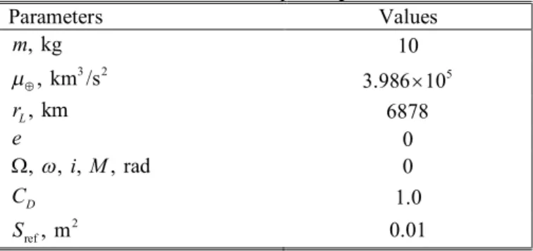
formation radius, i.e.,  ₀ 1.0 km. The in-plane phase angle is assumed to be 0 degree ( 0 (deg)). The SFF system parameters and the orbital parameters of the leader satellite used for the numerical simulation are listed in Table 1, where C and D Sref are the drag coefficient and the cross sectional area of the follower satellite, respectively.

The disturbance force d

 

t acting on the follower satellite includes gravitational perturbations up to order and degree 10 and atmospheric drag. The atmospheric model is NRLMSISE-00. The selected date and time are January 1st_{, 2016 and 00:00:00 UTC. The parameters needed for the adaptive sliding mode controller are given by:}

1 1 4 , , 0.03, 0.026, 0.1, 0.05, 0.5 , 5 10 , 0.01 0.01 i i i i ki U Km U P P                (35)

where P is the orbital period of the leader satellite which is equal to 3

2 L / 94.6135 (min)

P  r   .

The initial states for the numerical simulation are determined by substituting t 0 into Eq. (4) with a 1 km position offset on each axis. The initial velocity components are obtained by taking the time derivative of Eq. (4) and substituting t 0. Accordingly, the initial conditions for the relative state are given by:

 

0 



1000 2000 1000



T (m),

 

0 



0.5534 0 1.1068



T (m/s).

q q (36)

Figure 1 shows relative position errors and control thrust histories for formation keeping. The control thrusts are

saturated at 3

/ 5 10 N/kg

U m 

  . Although there is a 1 km initial position offset on all three axes and the maximum magnitude of the control input is limited, it is observed that the position errors are rapidly decreased to the vicinity of zero. More specifically, it is obtained that the final errors in each axis are e x 5.127 (mm), e y 0.03472 (mm),

and e z 0.03545 (mm). Obviously, these final errors can get smaller by reducing the value of  . The stabilization can be also viewed in the LVLH frame, plotted in Fig. 2. In the left, the controlled and reference trajectories are plotted in the y-z plane and the same trajectories are plotted in the x-z plane in the right. As expected from Eq. (4), the reference trajectory is a circle in the y-z plane and a straight line in the x-z plane. Despite the initial misalignment, the controlled trajectory is gradually merged into the desired reference trajectory.

Figure 3 shows the time histories of the sliding variables in each axis. From the definition of Eq. (6), s_i

 

0 0 holds, so that the reaching phase is removed and the robustness is guaranteed from the beginning. Immediately,

 

i

s t steeply rises because the control input is saturated at its maximum. However, it starts to decrease in a finite time and becomes bounded by the desired region si  from around t 0.15 (period) at which the control input is

relaxed from saturation (See Fig. 1).

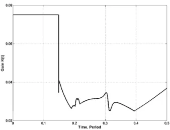
The adaptive gain K t

 

updated by Eq. (23) is depicted in Fig. 4. According to Eq. (24), it has its minimum 0.25

m

K  and its maximum UKm0.75. K t

 

maintains its maximum while the control input is saturated. When saturation is released, the gain K t

 

is computed as the sum of max



ux,uy,uz



and the margin K . m

Table 1 Orbital and system parameters

Parameters Values , kg m 10 3 2 , km /s _ 5 3.986 10 , km L r 6878 e 0 , , ,  i M, rad  0 D C 1.0 2 ref, m S 0.01

Fig. 1 Relative position errors and control thrust histories

Fig. 2 Controlled and desired trajectories in the y-z plane (left) and x-z plane (right) of the LVLH frame

Fig. 3 Time histories of the sliding variables

Fig. 4 Time history of the gain K t

 

V. Conclusions

In this paper, an adaptive robust control scheme based on the concept of global SMC is proposed to precisely control a multiple SFF system. The proposed controller effectively avoids chattering and successfully overcomes the effects of the uncertainties in the mass of the follower satellite and the external disturbances to which the satellite may be subjected. The adaptive gain update law, which only uses the measurement of the control input in the previous time step, eliminates the necessity of exact estimations of the uncertain bounds. Compared with existing adaptive SMC approaches, the proposed one is much simpler in that it requires only one positive number (K ) as an m

input parameter in the adaptive law. Numerical simulations that take into account an uncertain mass of the follower satellite and uncertain space environment caused by gravitational perturbations and atmospheric drag are carried out to demonstrate the strength of the proposed control scheme and the gain update law, which shows that a finite-time convergence to the desired target area with allowed error bounds is attained despite initial offset errors and along with the severe uncertainties.

References

1_{Aoude, G. S., How, J. P., and Garcia, I. M., “Two-Stage Path Planning Approach for Designing Multiple Spacecraft} Reconfiguration Maneuvers,” Proceedings of the 20th International Symposium on Space Flight Dynamics, NASA CP-2007-214158, Greenbelt, MD, 2007, pp. 1–16.

2_{Hill, G. W., “Researches in the Lunar Theory”, American Journal of Mathematics, Vol. 1, No. 1, 1878, pp. 5-26.}

3_{Clohessy, W. H. and Wiltshire, R. S., “Terminal Guidance System for Satellite Rendezvous,” Journal of Aerospace}

Sciences, Vol. 27, No. 8, 1960, pp. 653-658.

4_{Tschauner, J. and Hempel, P., “Rendezvous zu Einemin Elliptischer Bahn Umlaufenden Ziel,” Astronautica Acta, Vol. 11,} No. 2, 1965, pp. 104-109.

5_{Yan, Q., Kapila, V., and Sparks, A. G., “Pulse-Based Periodic Control for Spacecraft Formation Flying,” American Control}

Conference, Chicago, Illinois, June 2000, pp. 374-378.

6_{Won, C. H. and Ahn, H. S., “Nonlinear Orbital Dynamic Equations and State-Dependent Riccati Equation Control of} Formation Flying Satellites,” Journal of the Astronautical Sciences, Vol. 51, No. 4, 2003, pp. 433-449.

7_{Wong, H., Kapila, V., and Sparks, A., “Adaptive Output Feedback Tracking Control of Multiple Spacecraft,” American}

Control Conference, Arlington, VA, June 2001.

8_{Wu, C., and Chen, B., “Adaptive Attitude Control of Spacecraft Mixed H}

2/H∞ Approach,” Journal of Guidance, Control,

and Dynamics, Vol. 24, No. 4, 2001, pp. 755-767.

9_{Utkin, V., Guldner, J., and Shi, J., Sliding Modes in Electromechanical Systems, Taylor and Francis, London, 1999, pp. 147–} 153.

10_{Isidori, A., Nonlinear Control Systems, 3rd ed., Springer-Verlag, London, 1995.}

11_{Yeh, H., Nelson, E., and Sparks, A., “Nonlinear Tracking Control for Satellite Formations,” Journal of Guidance, Control,}

and Dynamics, Vol. 25, No. 2, 2002, pp. 376-386.

12_{Varma, S. and Kumar, K. D., “Multiple Satellite Formation Flying Using Differential Aerodynamic Drag,” Journal of}

Spacecraft and Rockets, Vol. 49, No. 2, 2012, pp. 325-336.

13_{Burton, J. A. and Zinober, A. S., “Continuous Approximation of Variable Structure Control,” International Journal of}

Systems Science, Vol. 17, No. 6, 1986, pp. 875–885.

14_{Li, M., Wang, F., and Gao, F., “PID-Based Sliding Mode Controller for Nonlinear Processes,” Industrial and Engineering}

Chemistry Research, Vol. 40, No. 12, 2001, pp. 2660-2667.

15_{Massey, T., and Shtessel, Y., “Continuous Traditional and High-Order Sliding Modes for Satellite Formation Control,”}

Journal of Guidance, Control, and Dynamics, Vol. 28, No. 4, 2005, pp. 826–831.

16_{Udwadia, F. E., Wanichanon, T., and Cho, H., “Methodology for Satellite Formation-keeping in the Presence of System} Uncertainties,” Journal of Guidance, Control, and Dynamics, Vol. 37, 2014, pp. 1611-1624.

17_{Godard and Kumar, K. D., “Fault Tolerant Reconfigurable Satellite Formations Using Adaptive Variable Structure} Techniques,” Journal of Guidance, Control, and Dynamics, Vol. 33, 2010, pp. 969-984.

18_{Liu, L., Han, Z., and Li, W., “Global Sliding Mode Control and Application in Chaotic Systems,” Nonlinear Dynamics,} Vol. 56, 2009, pp. 193-198.

19_{Sabol, C., Burns, R., and McLaughlin, C., “Satellite Formation Flying Design and Evolution,” Journal of Spacecraft and}

Rockets, Vol. 38, No. 2, 2001, pp. 270-278.

20_{Cho, H., and Udwadia, F. E., “Explicit Solution to the Full Nonlinear Problem for Satellite Formation-Keeping,” Acta}

Astronautica, Vol. 67, Nos. 3–4, 2010, pp. 369–387.

21_{Vallado, D. A., Fundamentals of Astrodynamics and Applications, 1st Ed., The McGraw-Hill Companies, Inc., Hawthorne,} CA, 1997, pp. 37-39.

22_{Cho, H., and Yu, A., “New Approach to Satellite Formation-Keeping: Exact Solution to the Full Nonlinear Problem,”}

Journal of Aerospace Engineering, Vol. 22, No. 4, 2009, pp. 445–455.