HAL Id: hal-01355262
https://hal.inria.fr/hal-01355262
Submitted on 22 Sep 2016
HAL is a multi-disciplinary open access
archive for the deposit and dissemination of
sci-entific research documents, whether they are
pub-lished or not. The documents may come from
teaching and research institutions in France or
abroad, or from public or private research centers.
L’archive ouverte pluridisciplinaire HAL, est
destinée au dépôt et à la diffusion de documents
scientifiques de niveau recherche, publiés ou non,
émanant des établissements d’enseignement et de
recherche français ou étrangers, des laboratoires
publics ou privés.
Time-Series Constraints: Improvements and Application
in CP and MIP Contexts
Ekaterina Arafailova, Nicolas Beldiceanu, Rémi Douence, Pierre Flener, María
Andreína Francisco Rodríguez, Justin Pearson, Helmut Simonis
To cite this version:
Ekaterina Arafailova, Nicolas Beldiceanu, Rémi Douence, Pierre Flener, María Andreína Francisco
Rodríguez, et al.. Time-Series Constraints: Improvements and Application in CP and MIP Contexts.
CPAIOR 2016 - 13th International Conference on Integration of Artificial Intelligence and Operations
Research Techniques in Constraint Programming, May 2016, Banff, Canada. pp.18-34,
�10.1007/978-3-319-33954-2�. �hal-01355262�
Time-Series Constraints: Improvements and
Application in CP and MIP Contexts
Ekaterina Arafailova1, Nicolas Beldiceanu1, Rémi Douence1, Pierre Flener2,
María Andreína Francisco Rodríguez2, Justin Pearson2, and Helmut Simonis3 1 TASC/ASCOLA (CNRS/INRIA), Mines Nantes, FR – 44307 Nantes, France
{Ekaterina.Arafailova,Nicolas.Beldiceanu,Remi.Douence}@mines-nantes.fr
2 Uppsala University, Dept of Information Technology, SE – 751 05 Uppsala, Sweden
{Pierre.Flener,Maria.Andreina.Francisco,Justin.Pearson}@it.uu.se
3 Insight Centre for Data Analytics, University College Cork, Ireland
Abstract. A checker for a constraint on a variable sequence can often be compactly specified by an automaton, possibly with accumulators, that consumes the sequence of values taken by the variables; such an automaton can also be used to decompose its specified constraint into a conjunction of logical constraints. The inference achieved by this de-composition in a CP solver can be boosted by automatically generated implied constraints on the accumulators, provided the latter are updated in the automaton transitions by linear expressions. Automata with non-linear accumulator updates can be automatically synthesised for a large family of time-series constraints. In this paper, we describe and evaluate extensions to those techniques. First, we improve the automaton synthe-sis to generate automata with fewer accumulators. Second, we decompose a constraint specified by an automaton with accumulators into a conjunc-tion of linear inequalities, for use by a MIP solver. Third, we generalise the implied constraint generation to cover the entire family of time-series constraints. The newly synthesised automata for time-series constraints outperform the old ones, for both the CP and MIP decompositions, and the generated implied constraints boost the inference, again for both the CP and MIP decompositions. We evaluate CP and MIP solvers on a prototypical application modelled using time-series constraints.
1
Context and Motivation
Frameworks are given in [4,14] for specifying a constraint on a sequence of vari-ables in a high-level way by means of a finite automaton, possibly augmented with accumulators in the framework of [4]. An automaton can be seen as a checker for ground instances of the specified constraint. For example, in a nono-gram puzzle, a row constrained to contain two stretches of black cells, of lengths 4 and 3 in this order, separated by at least one white cell but preceded and followed by any amounts of white cells, can be checked by an automaton equiv-alent to the regular expression w∗b4w+b3w∗, where the row is represented by a
Accumulators enable the specification of a constraint γ on a variable sequence X by an automaton whose size does not depend on the length of X: accumulators are initialised at the start state and are updated through the transitions; upon acceptance, the accumulators are linked to another variable of γ via an arith-metic constraint. For example, one could constrain the number of white cells between the two black stretches in the nonogram constraint above to be at most half the length of the row.
The framework of [14] lifts an automaton without accumulators into a propa-gator for the specified constraint; it maintains domain consistency in polynomial time. The more general framework of [4] lifts an automaton, possibly with accu-mulators, into a decomposition of the specified constraint in terms of constraints with existing propagators; in the presence of accumulators, this decomposition does not maintain domain consistency in general [2]. Encoding the potential ac-cumulator values in the states of the automaton may lead to an exponentially large automaton. In this paper, we focus on automata with accumulators.
The propagation achieved by the automaton decomposition of [4] in a CP solver can be boosted by invariants, seen as implied constraints, on the accumula-tors. If the latter are updated in the automaton transitions by linear expressions on the accumulators — such as increments and decrements by constant amounts (as in c := c + 1) or by other accumulators (as in c := c + r), or resets (as in c := 0) — then such implied constraints can be automatically generated [11].
Automata with non-linear accumulator updates can be automatically syn-thesised for a large family of structural time-series constraints [3]. A time se-ries is here a sequence of integers, corresponding to measurements taken over a time interval. Time series are common in many application areas, such as the power output of electric power stations over multiple days, or environmental data (temperature, humidity, CO2level) in buildings. Time series are constrained by
physical or organisational limits, which restrict the evolution of the series. After a summary of the background material in Section 2, the contributions and impact of this paper are as follows:
– We improve the automated automaton synthesis of [3] so as to synthesise automata with fewer accumulators and simpler accumulator updates, using fewer ‘min’ and ‘max’ operators, say (Section 3).
– We decompose a constraint specified by an automaton with accumulators into a linear-sized conjunction of linear inequalities, for use by a mixed-integer programming (MIP) solver (Section 4).
– We generalise the implied constraint generation of [11] so as to cover the en-tire family of time-series constraints of [3] and to rank the generated implied constraints by decreasing propagation strength, thereby easing the human selection of which implied constraints actually to use (Section 5).
– We show that the newly synthesised automata for time-series constraints outperform the automata of [3], for both the CP and MIP decompositions, and that the newly generated implied constraints boost the inference, again for both the CP and MIP decompositions (Section 6).
– We evaluate CP and MIP solvers on a prototypical application modelled with the help of time-series constraints (Section 7).
2
Specifying (Time-Series) Constraints using Automata
We showed in [3] that many constraints γ(N, hX0, . . . , Xn−1i) on an unknowntime series hX0, . . . , Xn−1iof given length n can be specified as a triple hp, f, gi,
where p is a regular expression over the alphabet {<, =, >} and is called the pattern; f ∈ {max, min, one, range, surface, width} is called the feature; and g ∈ {Max, Min, Sum} is called the aggregator. The semantics is that integer variable N is required to be the aggregation, computed using g, of the list of features f of all maximal words matching p within the sequence hS0, . . . , Sn−2i
of variables, called the signature sequence, which is linked to the time series via the signature constraints (Xi < Xi+1 ⇔ Si = ‘<’) ∧ (Xi = Xi+1 ⇔ Si =
‘=’) ∧ (Xi > Xi+1 ⇔ Si=‘>’) for all i ∈ [0, n − 2]. A list of 23 patterns was
identified, giving 266 constraints. We now introduce our running example. Example 1. The MaxWidthStrictlyDecreasingSequence(N, X) constraint, requiring N to be the maximum width of the maximal strictly decreasing se-quences within the time series X, is specified by the pattern >+, the feature
width, and the aggregator Max. The time series h4, 4, 3, 2, 2, 6, 3, 5i contains two maximal strictly decreasing sequences, namely 4 > 3 > 2 and 6 > 3, of widths 3 and 2, so their maximum width is N = 3. The following figure shows how to check MaxWidthStrictlyDecreasingSequence(3, h4, 4, 3, 2, 2, 6, 3, 5i) by (I) build-ing the signature sequence by comparbuild-ing adjacent time-series values; (II) findbuild-ing all maximal words matching the regular expression >+; (III) computing the
fea-ture width of each such strictly decreasing sequence; and (IV) aggregating the feature values using the Max aggregator:
Max width >+ 0 1 2 3 4 5 6 7 4 4 3 2 2 6 3 5 = > > = < > < > > >> >> 3 2 3 1 2 3 5 6 time series
(I) signature sequence
(II) maximal occurrences (III) feature sequence (IV) feature aggregation
An automaton with a memory of m ≥ 0 integer accumulators [4] is a tuple hQ, Σ, δ, q0, I, A, αi, where Q is the set of states, Σ the alphabet, δ : (Q × Zm) ×
Σ → Q × Zm the transition function, q
0 ∈ Q the start state, I the m-tuple
of initial values of the accumulators, A ⊆ Q the set of accepting states, and α : Zm→ Z the acceptance function, transforming the memory of an accepting state into an integer. If the left-to-right consumption of the symbols of a word win Σ∗ transits from q0 to some accepting state and the m-tuple C of current
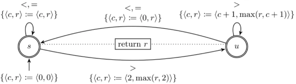
accumulator values, then the automaton returns the value α(C), else it fails. Example 2. A ground instance of the constraint of Example 1 holds if and only if its value of N is returned by the automaton in Figure 1 after consuming the signature sequence linked to its time series X. The automaton uses m = 2 accu-mulators: at any moment, accumulator c has the length of the current strictly decreasing sequence, while r has the length of the longest strictly decreasing
s {hc, ri := h0, 0i} u return r > {hc, ri := h2, max(r, 2)i} <, = {hc, ri := hc, ri} > {hc, ri := hc + 1, max(r, c + 1)i} <, = {hc, ri := h0, ri}
Fig. 1: Automaton for MaxWidthStrictlyDecreasingSequence
sequence seen so far. The state set Q is {s, u}: at s the current sequence is not strictly decreasing, and at u the current sequence is strictly decreasing. The start state q0= sis indicated by an arc coming from nowhere, annotated within
braces by the initialisation to zero of both c and r, hence I = h0, 0i. The al-phabet Σ is {<, =, >}. The arc from s to u depicts the transition of δ from s to u upon consuming symbol >, and is annotated within braces by accumulator updates: r is updated to its maximum with 2, and c is set to 2. All states are accepting, hence A = Q. The acceptance function α transforms a memory hc, ri into r at both states, and is given in a box linked to s and u by dotted lines. ut
An automaton can be seen as a constraint checker. The framework of [14] lifts an automaton with m = 0 accumulators into a CP propagator for the specified constraint; it maintains domain consistency in time polynomial in the automaton size and sequence length. The more general framework of [4] lifts an automaton with m ≥ 0 accumulators into a CP decomposition of the specified constraint in terms of constraints with existing CP propagators; when m ≥ 1, this decomposi-tion does not maintain domain consistency in general [2]. Encoding the potential accumulator values in the states of the automaton, so as to get an automaton with m = 0 accumulators, may lead to a large automaton.
In this paper, we focus on automata with m ≥ 1 accumulators, motivated [4] by the wish to specify a constraint on a sequence X by an automaton whose size does not depend on the length of X; this is the case for the automaton in Figure 1. In Section 3, we improve our synthesiser [3] of automata from hp, f, gi specifications of time-series constraints, so that it automatically synthesises au-tomata with fewer accumulators and simpler accumulator updates, namely linear accumulator updates rather than updates involving the min and max operators. In Section 4, we lift an automaton with m ≥ 1 accumulators into a MIP decom-position of linear inequalities. In Section 5, we boost the inference achieved for the CP and MIP decompositions by generalising our generator [11] of constraints implied by an automaton, so that it covers the entire family of time-series con-straints of this section and [3]. Those sections are orthogonal and any subset thereof can be read in any sequence.
3
Simplification of Synthesised Time-Series Automata
In [3] we synthesise automatically an automaton from a triple hp, f, gi specifying a time-series constraint. The synthesis relies on a declarative encoding of proce-dural knowledge into what we call decoration tables [3]. Each pattern is specified by a transducer [6,15] obeying wellformedness conditions. The decoration tables are parametrised by features and aggregators, and define substitution rules on the transducers that allow an automaton with m = 3 accumulators to be syn-thesised. The future work in [3] included simplifying the synthesised automata, as they often have more accumulators and more complex accumulator updates than manually designed ones: this may slow down the checker and weaken CP or MIP decompositions of the constraint specified by the synthesised automaton.In this paper, we largely overcome this bottleneck. Rather than designing a procedural minimisation algorithm for automata with accumulators, we have again opted for capturing such procedural knowledge in a declarative and thus more easily reusable way: it suffices to specialise the decoration tables of [3] for some combinations of algebraic properties of pattern-feature-aggregator triples. First, we recall the concept of pattern e-occurrence from [3], capturing where a feature value is extracted from the time series.
Definition 1. Given a pattern p; a sequence X0, . . . , Xn−1; its signature
se-quence S0, . . . , Sn−2; and a non-empty subsequence Si, Si+1, . . . , Sj forming a
maximal word that matches p, with 0 ≤ i ≤ j ≤ n − 2; the e-occurrence of that maximal word is the interval [`, u] of corresponding indices within X0, . . . , Xn−1.
In Example 1, the sequence X = h4, 4, 3, 2, 2, 6, 3, 5i gives the signature se-quence S = h=, >, >, =, <, >, <i, which contains two maximal words matching the pattern >+ of strictly decreasing sequences, namely hS
1, S2i = h>, >iand
hS5i = h>i, corresponding to the strictly decreasing sequences hX1, X2, X3i =
h4, 3, 2iand hX5, X6i = h6, 3i, hence the e-occurrences are [1, 3] and [5, 6]. A
pat-tern occurrence hSi, . . . , Sjiwithin the signature sequence has the e-occurrence
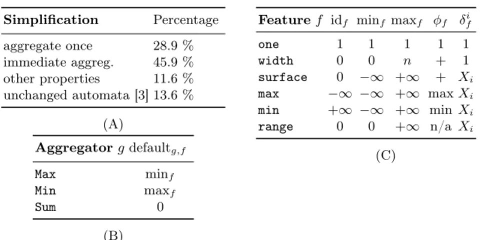
[i, j + 1]for this constraint, but it could be [i + 1, j] for other constraints [3]. All synthesised automata in [3] have the accumulators c, d, and r, which respectively denote the feature value of the current pattern e-occurrence (such as accumulator c in Figure 1); the feature value of a potential part of a pattern e-occurrence (no such accumulator is needed in Figure 1, and achieving this is the purpose of this section); and the aggregated result value for the feature val-ues of the pattern e-occurrences already encountered (such as accumulator r in Figure 1). Figure 2B&C gives the functions used to compute the feature and aggregation values. If the pattern, feature, and aggregator satisfy some proper-ties, then either it is enough to perform the accumulator update only on one specific transition of the automaton, as in Definition 3, or it is possible to start aggregating immediately upon finding an e-occurrence, as in Definition 4. To state these properties, we need another concept.
Definition 2. A transition from state q to state q0 in an automaton is called a ‘found’ transition if it is the only transition on some path from the initial state q0
Simplification Percentage aggregate once 28.9 % immediate aggreg. 45.9 % other properties 11.6 % unchanged automata [3] 13.6 % (A) Aggregator g defaultg,f Max minf Min maxf Sum 0 (B)
Feature f idf minf maxf φf δif
one 1 1 1 1 1 width 0 0 n + 1 surface 0 −∞ +∞ + Xi max −∞ −∞ +∞ max Xi min +∞ −∞ +∞ min Xi range 0 0 +∞ n/a Xi (C)
Fig. 2: (A) Percentage, among the 266 time-series constraints, of automata that can be simplified using the discovered properties. (C) Features: their identity, minimum, and maximum values; the functions φf and δif are used to compute
recursively the feature value vu of a sequence hX`, . . . , Xuiby v` = φf(idf, δf`)
and vi= φf(vi−1, δif)for i > `; note that δfi provides the contribution of Xi to
the value of feature f; (B) Aggregators and their default values.
For example, the transition from the start state s to state u in Figure 1 is a ‘found’ transition, as it sets c to 2.
Definition 3. Given a time-series constraint γ on feature f , an e-occurrence [`, u] of its pattern such that Xs triggers a ‘found’ transition of its
automa-ton, with s ∈ [`, u], we say that γ is an aggregate-once constraint if δs f equals
φf(φf(. . . φf(idf, δf`), . . . , δ u−1
f ), δ
u
f), where φf and δfi are as in Figure 2B.
For aggregate-once constraints the feature value of an e-occurrence depends only on the value of δs
f, hence we need only one counter for aggregating.
For example, any constraint with feature f = one, i.e., any constraint count-ing the number of occurrences of a pattern, is an aggregate-once constraint, because for any e-occurrence [`, u] and any i, i+1 ∈ [`, u] we have φf(δif, δ
i+1
f ) =
δ`f = δf`+1= · · · = δfu= 1. Also, consider any constraint with feature f = max and pattern ‘<(<|=)*(>|=)*>’, which means there is a strict increase followed by a non-strictly increasing subsequence, possibly a plateau, and then a non-strictly decreasing subsequence, followed by a strict decrease. The maximal value δs
f of an
e-occurrence [`, u] of that pattern is found already when we traverse the ‘found’ transition for s ∈ [`, u], which is the first transition on signature symbol ‘>’: there is no need then to consider other elements of the e-occurrence because the rest of the pattern is a non-strictly decreasing sequence, so we can aggregate once we know δs
f. Formally, such a constraint is an aggregate-once constraint, because
for any e-occurrence [`, u] we have that φf(φf(. . . φf(idf, δ`f), . . . , δ u−1
f ), δ
u
max(idf, δf`, . . . , δ u
f) = max(idf, Xf`, . . . , X u
f) = Xs = δfs, where Xs triggers a
‘found’ transition of the automaton, with s ∈ [`, u].
The second kind of time-series constraints, in Definition 4 below, is char-acterised by a combination of feature and pattern properties for which we can start aggregating a current feature value into the result accumulator r as soon as when we find out that we are within a pattern e-occurrence, i.e., without waiting for the end of that pattern e-occurrence. To understand how a synthesised au-tomaton works, we define the following functions, parametrised by entries from Figure 2B&C, representing the updates of the accumulators c and r:
– Ff : Z × Z → Z × Z (ci, ri) 7→ (φf(ci, δfi), ri)
– G0f,g: Z × Z → Z × Z (ci, ri) 7→ (idf, g(ri, φf(ci, δif)))
– G00f,g: Z × Z → Z × Z (ci, ri) 7→ (φf(ci, δfi), g(ri, φf(ci, δfi)))
When a synthesised automaton from [3] computes the value of feature f for an e-occurrence [`, u] and aggregates it into the result accumulator r, the new value of r is computed by first applying u − ` times the function Ff and then applying
the function G0
f,g. However it is often possible to aggregate this feature value into
rwithout waiting for the end of the e-occurrence. There are two such situations: either (a) before aggregating, we must evolve the feature value of the e-occurrence in accumulator c; or (b) we need not evolve this feature value in c, but after each aggregation c is reset to the idf value from Figure 2B. We apply u − ` times the
function G00
f,g or G
0
f,gfor the situations (a) and (b) respectively. Finally G 0
f,g is
applied once for both (a) and (b), since we do not have to keep in accumulator c the feature value when we are at the end of the e-occurrence. The old [3] order of accumulator updates corresponds to G0
f,g◦ Ff◦ · · · ◦ Ff, called order (1), while
the new order of updates corresponds to either G0
f,g◦ G0f,g◦ · · · ◦ G0f,g, called
order (2), or G0
f,g◦ G00f,g◦ · · · ◦ G00f,g, called order (3).
Definition 4. A time-series constraint is an immediate-aggregation constraint if for any e-occurrence the use of order (1) has the same result as using either order (2) or order (3).
Due to the immediate-aggregation property, we do not have to distinguish the potential and current parts anymore. In [3], updating r is done after the end of an e-occurrence, taking into account the current feature value in c. However, we need not aggregate after the end of an e-occurrence, as the update of r should happen when we are sure that the current element Xi belongs to the
e-occurrence, so we can use c for keeping both the potential and current parts. For example, the MaxWidthStrictlyDecreasingSequence constraint is an immediate-aggregation constraint. This is illustrated in Figure 3, where ci
and rirespectively denote the values of accumulators c and r after consuming Xi:
we consider an e-occurrence [`, u] and apply the two orders (1) and (3); after the last update, the value of the accumulator r coincides for both orders. The column ‘before’ contains the value of the accumulators just before the e-occurrence [`, u]. The simplified automaton for this constraint is given in Figure 1.
The percentage of constraints for which we can simplify the automata using the different types of simplifications is given in Figure 2A.
before update 1 · · · update u − ` update u − ` + 1 order (1)
c update c`= c`−1+ 1 · · · cu−1= cu−2+ 1 cu= 0
r update r`= r`−1 · · · ru−1= ru−2 ru= max(ru−1, cu−1+ 1)
(c, r) (0, r`−1) (1, r`−1) · · · (u − `, r`−1) (0, max(r`−1, u − ` + 1))
order (3)
c update c`= c`−1+ 1 · · · cu−1= cu−2+ 1 cu= 0
r update r`= max(r`−1, c`−1+ 1) · · · ru−1= max(ru−2, cu−2+ 1) ru= max(ru−1, cu−1+ 1)
(c, r) (0, r`−1) (1, max(r`−1, 1)) · · · (u − `, max(r`−1, u − `)) (0, max(r`−1, u − ` + 1))
Fig. 3: MaxWidthStrictlyDecreasingSequence immediately aggregates
4
MIP Decomposition of Automaton-Based Constraints
Consider a constraint γ(N, hX0, . . . , Xn−1i)and signature constraints linking itsnvariables Xj to n + 1 − w signature variables Si, each Sibeing functionally
de-termined by a linear relation on w consecutive Xj variables. For ease of notation,
we here assume w = 2: each Si is linked to Xi and Xi+1, as for the time-series
constraints in Section 2. (Other frequent scenarios are w = 1, where each Si is
linked to Xi only, and the absence of signature constraints, in which case one
would assume Si= Xi are the signature constraints, also with w = 1.)
Assume a ground instance of γ(N, hX0, . . . , Xn−1i)holds iff an automaton A
with m ≥ 1 accumulators aj that are updated by linear expressions φ, possibly
using the ‘max’ and ‘min’ operators, returns the value of its variable N, called the result variable, after consuming the values of its signature variables S0, . . . , Sn−2.
Following [1], we decompose γ for a MIP solver by formulating logical con-straints that model the triggering of transitions in A (Section 4.1) and linearising those constraints (Section 4.2). For m = 0, there is the flow-based MIP decom-position of [8]. For m = 1 accumulator that is only updated through increments by positive integers, there is the column-generation approach of [9].
4.1 Logical Constraints
Beside the integer variables X0, . . . , Xn−1and N of γ, to model the behaviour of
A = hQ, Σ, δ, q0, I, A, αion the signature variables S0, . . . , Sn−2over Σ, the key
idea is to represent the states visited by A using state variables Q0, . . . , Qn−1
over Q: each Qidenotes the state reached after consuming Si−1, with Q0= q0.
Also, we need transition variables T0, . . . , Tn−2 over the set T = Q × Σ of
constants denoting all the transitions of the total function δ: each Tidenotes the
(i + 1)st triggered transition of A, that is while consuming S i.
Last, we need accumulator variables Ai,jfor i ∈ [0, n−1] and j ∈ [1, m]: each
integer Ai,j denotes the value of accumulator aj after the ith transition of A,
that is after consuming Si−1; each A0,j is given in the tuple I of initial values.
The signature constraints functionally determine each signature variable Si
from a linear relation on Xi and Xi+1. For example, the signature constraints
The transition constraints encode the transitions of δ as follows: Q0= q0
Qi= q ∧ Si= σ ⇒ Qi+1= δ(q, σ) ∧ Ti= hq, σi, ∀i ∈ [0, n − 2], ∀q ∈ Q, ∀σ ∈ Σ
For example, a representative transition constraint for the automaton of Figure 1 is: Qi= s ∧ Si=‘<’ ⇒ Qi+1= s ∧ Ti= hs, <i, ∀i ∈ [0, n − 2].
The accumulator constraints are of three kinds: the values of the accumulator variables A0,j before any transitions are found in the m-tuple I of initial values;
there is an implication constraint for each transition of δ with its accumulator updates; and the values of the accumulator variables An−1,j after all transitions
are linked to the result variable N according to the acceptance function α. If A ( Q, then we have to pose the additional constraint Qn−1∈ A.
For example, the accumulator constraints for the automaton in Figure 1 are as follows, using the accumulator variables Ciand Lifor denoting the successive
values of the accumulators c and ` respectively: the constraints L0= 0and C0=
0 correspond to the pair I = h0, 0i of initial values; the constraint N = Ln−1
stems from the acceptance function; further:
Ti= t ⇒ Ci+1= Ci, ∀t ∈ {hs, <i, hs, =i} , ∀i ∈ [0, n − 2]
Ti= hs, >i⇒ Ci+1= 2, ∀i ∈ [0, n − 2]
Ti= t ⇒ Ci+1= 0, ∀t ∈ {hu, <i, hu, =i} , ∀i ∈ [0, n − 2]
Ti= hu, >i⇒ Ci+1= Ci+ 1, ∀i ∈ [0, n − 2]
Ti= t ⇒ Li+1 = Li, ∀t ∈ {hs, <i, hs, =i, hu, <i, hu, =i} , ∀i ∈ [0, n − 2]
Ti= hs, >i⇒ Li+1 = max(Li, 2), ∀i ∈ [0, n − 2]
Ti= hu, >i⇒ Li+1 = max(Li, Ci+ 1), ∀i ∈ [0, n − 2]
For n variables Xi and m accumulators, there are n − 1 signature variables,
nstate variables, n−1 transition variables, and mn accumulator variables, hence Θ(n)variables in total, since m is a constant. Since A has a constant size, each variable occurs in a constant number of constraints, so there are Θ(n) constraints.
4.2 Linearising the Logical Constraints
To obtain a linear model, we linearise each group of logical constraints.
For each variable Si over Σ, we introduce 0-1 variables Sσi, with 1 denoting
truth and 0 denoting falsity, hence the semantics Sσ
i = 1 ⇔ Si = σ for all
i ∈ [0, n − 2]and σ ∈ Σ. This requires that exactly one of the Sσ
i takes value 1:
X
σ∈Σ
Siσ= 1, ∀i ∈ [0, n − 2] (1)
We replace each atom Si= σby the Boolean Sσi in each logical constraint.
We perform the same operation for the Qi and Ti variables with respect to
their domains, getting variables Qq
i and Tit for all q ∈ Q and t ∈ T . If A ( Q,
then we additionally require Qq
To linearise the transition constraints, which are now implications where both sides are conjunctions of Boolean variables, we use the technique of [17, pages 172–177].
The accumulator constraints have the general logical form
Ti= t ⇒ Ai+1,j = φ, with i ∈ [0, n − 2], j ∈ [1, m], and t ∈ T
where φ is here a linear expression, possibly using the ‘max’ and min’ operators, that mentions variables Ai,j denoting accumulator values before the considered
ith transition. We linearise such an implication as follows:
Ai+1,j− φ ≤ Mj· (1 − Tit), with i ∈ [0, n − 2], j ∈ [1, m], and t ∈ T
Ai+1,j− φ ≥ Mj· (Tit− 1), with i ∈ [0, n − 2], j ∈ [1, m], and t ∈ T
where constant Mj, chosen with respect to the function φ, is such that the
constraints above always hold. Computation of Mj may also require calculation
of the values serving as plus and minus infinities. For example, for a time-series constraint specified by a triple hp, f, gi, we have that each Mj depends on the
extrema of feature f. If φ uses the ‘max’ and min’ operators, then we first linearise it using the technique of [10, pages 4–5], introducing a constant number of new variables.
We linearise the signature constraints by using the following technique, ex-plained on the example of time-series constraints, where the minimum difference between two consecutive integer variables Xi is 1. We rewrite the signature
con-straint Xi < Xi+1 ⇔ Si =‘<’ as two linear inequalities enforcing Si< = 1 if
Xi< Xi+1, and Si<= 0 otherwise:
Xi+1− Xi Mi0 ≤ S < i ≤ Xi+1− Xi Mi0 + 2M0 i− 1 2Mi0 , ∀i ∈ [0, n − 2] where constant M0 i is max
v∈dom(Xi), w∈dom(Xi+1)
|w − v| + 1, for all i ∈ [0, n − 2], assuming dom(Y ) denotes the domain of variable Y . The linearisation of Xi>
Xi+1 ⇔ Si=‘>’ is symmetric. The linearisation of Xi= Xi+1 ⇔ Si=‘=’ is
Si<= 0 ∧ Si> = 0, since the instance S<i + S=
i + S
>
i = 1of (1) implies Si== 1.
For n variables Xi and m accumulators, there are (n − 1) · |Σ| signature
variables, n · |Q| state variables, (n − 1) · |Q| · |Σ| transition variables, and mn accumulator variables. Linearising any of the (n − 1) · |Q| · |Σ| accumulator constraints requires a constant number of new variables, if any. So we still have Θ(n) variables in total, since m, |Q|, and |Σ| are constants; for the time-series constraints, we have |Q| ≤ 4 for 240 of the 266 automata and |Q| ≤ 13 otherwise, m ≤ 3 upon the improvements in Section 3, and |Σ| = 3. Since each variable occurs in a constant number of constraints, there still are Θ(n) constraints.
5
Improved Generation of Implied Constraints
Given an automaton A with m ≥ 1 accumulators aj, our tool ImpGen [11]
hold at every state of A for any symbols consumed so far. Let variable Ai,jdenote
the value of accumulator ajafter A has consumed the first i symbols of a sequence
of n symbols: these variables appear in the CP decomposition [4], for a sequence of n variables Si, of the constraint specified by A. This decomposition in general
does not achieve domain consistency when m ≥ 1 [2]: achieving it is NP-hard for such a constraint in general [5]. Each invariant translates into n + 1 constraints of the form α1Ai,1+ · · · + αmAi,m+ γ ≥ 0, for all 0 ≤ i ≤ n. We showed in [11]
that these constraints are implied by the mentioned CP decomposition, and that the implied constraints translating a suitable selection of invariants improve the propagation strength and speed of that decomposition. The generation of implied constraints is specific to an automaton, but neither to a constrained sequence of variables Si nor to its length n, and can thus be done offline.
ImpGen handles automata where each accumulator update is a linear ex-pression on accumulators. This includes increments and decrements by constant amounts (as in c := c + 1) or other accumulators (as in c := c + `), resets (as in c := 0), etc. This excludes updates via the ‘max’ and ‘min’ operators, for instance: ImpGen handles only 64 of the 266 time-series constraints in Section 2. Towards handling all the time-series constraints, we need to extend ImpGen to handle also conditional accumulator updates of the form c := if ρ then φ else ψ, where ρ is a linear (in)equality and φ, ψ are linear expressions on accumulators: following an idea in [16], we extend the encoding of automaton transitions by allowing preconditions to be expressed. ImpGen now automatically first rewrites accumulator updates containing the binary ‘min’, ‘max’, or ‘abs’ operators into conditional updates. For example, the accumulator update on the arc from s to t in Figure 1 is rewritten as hc, `i := h2, if ` > 2 then ` else 2i.
Finally, we extend ImpGen to rank the implied constraints by decreasing propagation strength when added to the CP decomposition: this is done based on a series of random instances. This enables automated selection via a top-k rule for a user-chosen parameter k, as opposed to the previous manual selection among a set of implied constraints. For example, the top three implied constraints generated from the automaton in Figure 1 are Li ≥ Li−1, Li ≥ Li−2, and
Li+Li−1≥ 2·Li−2, where Lidenotes the value of accumulator ` after consuming
the first i symbols. The new tool is available online.1
Intuitively, the implied constraints generated by ImpGen can improve infer-ence also for the MIP decomposition of Section 4 because they are generated directly from an automaton and are not necessarily linear combinations of the linear inequalities in that decomposition [13]. Our experiments in the next sec-tion confirm that implied constraints that improve the propagasec-tion of the CP decomposition can also improve the inference of the MIP decomposition.
1
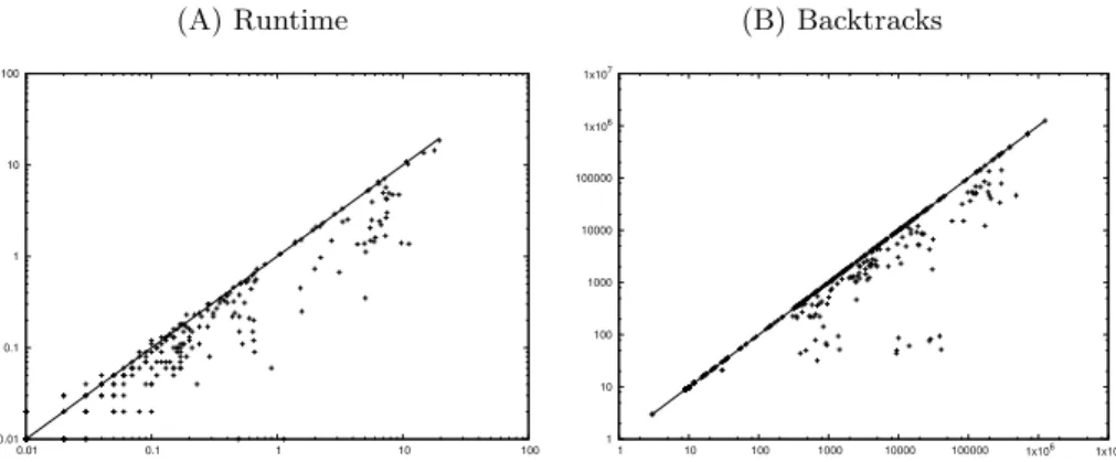
(A) Runtime 0.01 0.1 1 10 100 0.01 0.1 1 10 100 (B) Backtracks 1 10 100 1000 10000 100000 1x10⁶ 1x10⁷ 1 10 100 1000 10000 100000 1x10⁶ 1x10⁷
Fig. 4: Time in seconds (left) and backtracks (right) to maximise the result vari-able for random instances under SICStus Prolog 4.3.2 on a 2011 MacBook Pro 2.2 GHz quad-core Intel Core i7-950 machine with 6MB cache and 16 GB mem-ory. The x-axis is for the new automata and the y-axis is for the old automata: points below the diagonal represent good results for the new automata.
6
Benchmark on CP and MIP Solvers
To evaluate the CP and MIP decompositions of the time-series constraints, we compared their old automata [3] against the new automata of Section 3, and the new automata with and without implied constraints generated as in Section 5.
To compare the old automata against the new automata for CP, we generated instances for all the 266 time-series constraints over time series of length 15 over the domain {1, 2, 3}. Note that a domain of size 3 is large enough to allow all patterns to occur and to focus the propagation effort on the transition constraints and accumulator constraints but not on the signature constraints. We maximised the result variable, and used a timeout of 100 seconds. As can be seen in Figure 4, the decompositions of the new automata are almost always faster (actually 1.6 times faster on average) and always have fewer backtracks (actually 25% fewer backtracks on average) than those of the old automata.
To compare the new automata with and without implied constraints both for CP and MIP, we generated 40 instances for each constraint used in Section 7 below over time series of length 100 and random sub-intervals of [0, 1000] as domains. We maximised the result variable, and used a timeout of 300 seconds. Using SICStus Prolog [7], we chose a static search strategy, assigning the variables Xi by increasing index and trying values from smallest to largest.
This means that the first solution found is the same with and without implied constraints, and that the times and backtrack counts are directly comparable. The decompositions of the new automata are always faster in the presence of the top two implied constraints, namely 3.33 times faster on average, and always have fewer backtracks, by up to 5 orders of magnitude. In particular, all instances of half the constraints are now solved in less than 1 second instead of timing out.
Using the Gurobi 6.5 [12] MIP solver, the decompositions of the new au-tomata are almost always faster in the presence of the top two implied con-straints, namely also 3.33 times faster on average, and can solve to optimality 14% more instances. For the considered constraints, the decompositions of the new automata are always faster than those of the old automata, namely 1.63 times faster on average.
7
Evaluation on a Staff Scheduling Application
For a more realistic evaluation, we introduce a prototypical staff scheduling ap-plication that uses a number of time-series constraints. We consider the case of a service company, where demand varies over time, and has to be met at each time point. In order to provide the service level required, we have to define a manpower resource profile over time. Resource cost may vary over time, i.e., employees may be paid different rates at different times. If we could hire and fire personnel arbitrarily, we could follow the demand curve exactly, but this is not allowed, as business processes, employment rules, and union contracts limit how quickly we can change the number of persons employed. We are therefore required to sometimes employ more people than strictly necessary. Note that we are not dealing with a shift rostering problem, where the demand must be covered by people working different shift patterns. In the current problem we are only interested in the total manpower curve, over a long-term horizon.
The overall problem is to cover the given resource demand over time, while minimising overall resource cost, and at the same time satisfying the given time-series constraints.
7.1 Notation, Constants and Variables
In our benchmark, we use a time resolution of one week over a one year horizon, i.e. we consider n = 52 time points. The integer variables Xi describe the
sched-uled resource level at time i. These variables form a single time-series X1, ..., Xn,
all constraints are expressed over this time-series or over one of its sub-sequences. The symbols di define the given, fixed demand at each time point i. The
sym-bols ci define the cost of a resource unit at time point i. For each constraint we
also introduce an integer variable which represents the aggregated feature value for the constraint. The lower or upper domain bound of these variables will be constrained.
7.2 Objective Function
The objective is to minimise the total cost of the schedule, i.e.
obj∗= min
n
X
i=1
The overhead obj∗−Pn
i=1dici is the increase in cost due to the working rules.
We can use the overhead also to evaluate the potential cost/savings due to adding/removing a specific working rule. Another lower bound is the sum of the lower domain bounds after initial propagation: we use this to compute the finite-domain optimality gap in our evaluation.
7.3 Constraints
There are two types of constraints, one concerning the demand profile, and the other a set of time-series constraints. At each timepoint, the resources provided must exceed the required demand Xi≥ di.
The constraints on the time series are given in natural language form below, we also note the constraints used, following the naming scheme in [3].
1. The manpower profile can have at most two peaks. This is expressed with a NbPeak constraint with a parameter variable with an upper bound of two. 2. The manpower profile can have at most two valleys. This is handled by the
NbValley constraint.
3. The maximal manpower level at any peak of employment is 250. The num-bers employed at the start or end of the planning period can be higher. The MaxMaxPeak constraint handles this condition.
4. We can hire at most 5 persons in one week. This limit is caused by the in-duction training required. The inin-duction covers safety training, where spaces in each course are limited. We use the MaxRangeIncreasing constraint to model this condition.
5. We can fire at most 7 persons in one week (expressed with a MaxRangeDe-creasing constraint).
6. We can only have at most four consecutive increases of personnel in the planning period. This is expressed by the MaxWidthStrictlyIncreas-ingSequence constraint, considering that four consecutive increases lead to a pattern of width five.
7. We can only have at most six consecutive decreases of personnel numbers in the planning period (using MaxWidthStrictlyDecreasingSequence from Example 1).
8. If we reach a peak in the employment, the profile has to stay constant for at least 10 weeks. Otherwise, we will be violating a “hire and fire” union rule. This is handled by a MinWidthPlateau constraint.
9. If we fire a person, we can not hire another person for four weeks. Instead, we should keep on employing the person (MinWidthPlain).
10. We are not allowed to fire persons in the two weeks before Christmas (ex-pressed with a NbDecreasing constraint on a sub-sequence).
11. In every month, we can have at most 20 new hires. This is due to limitations of the human resources department. For this we use one SumRangeIn-creasing constraint for each month.
12. The difference between the highest and lowest peak should not be more than 30. We already have a MaxMaxPeak constraint to constrain the level of
the highest peak. A MinMaxPeak constrains the height of the lowest peak, an inequality between the parameters limits the difference to at most 30.
Manually generated redundant constraints In order to find solutions more easily, we initially manually defined some redundant constraints controlling the domain envelope. Constraint (4) can be approximated by inequalities Xi+1 ≤
Xi+ cwith a constant c equal to five (this is also generated by ImpGen), while
constraints (4) and (6) imply inequalities of the form Xi+p+1 ≤ Xi+ pc, as
any sequence of p + 1 intervals can contain at most p = 4 increases. These constraints are currently out of the scope of ImpGen because they are linear only at the instance level.
7.4 Search Routine and Experimental Setup
In order to evaluate the impact of different implementations of the constraints, we choose a static search strategy, assigning the Xi variables by increasing
in-dex, and enumerating values from smallest to largest. This means that the first solution found is the same for all CP models used, and the times and backtrack counts are directly comparable.
We create random sample problem instances that follow a common structure. There are demand peaks in Spring and Autumn, and reduced demand during Summer and Winter. The minimal difference between peaks and valleys is con-trolled by a parameter P , which we vary from 10 to 40 in steps of 5. For each parameter value, we generate 100 instances.
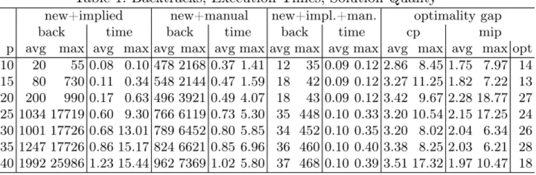
We compare different implementations of the time-series constraints, together with manually or automatically generated implied constraints, using the solvers described in Section 6, on the hardware introduced in Figure 4. On their own, the time-series constraints perform quite poorly. Both the old and the new automata definitions only solve instances for the easiest instance set (P=10), finding solu-tions for 12, respectively 16, of the 100 problems. Adding either manually defined constraints or the top two implied constraints as described in Section 5 to the new automata allow us to find solutions for all problem instances for all parame-ter values. Using the old automata with the manually defined constraints solves 90, 70, 45, 36, 31, 35, and 32 out of 100 instances for parameter values 10 to 40. For the combinations of automata and implied constraints that solve all in-stances we compare backtracks and solution times for the CP model in Table 1, which also shows the average and maximal optimality gap for both the CP and MIP models. Note that the finite-domain solver typically only finds a first solu-tion, and cannot prove optimality within the timeout period. We report results for finding that first solution. At the moment, the MIP solver, even when using the implied constraints and with a timeout of 300 seconds, only finds optimal solutions for some of the problem instances (column Opt), and performs worse than the CP model for some instances.
We can see that both automatically and manually generated implied con-straints are important, and that their combination significantly reduces the
Table 1: Backtracks, Execution Times, Solution Quality
new+implied new+manual new+impl.+man. optimality gap back time back time back time cp mip p avg max avg max avg max avg max avg max avg max avg max avg max opt 10 20 55 0.08 0.10 478 2168 0.37 1.41 12 35 0.09 0.12 2.86 8.45 1.75 7.97 14 15 80 730 0.11 0.34 548 2144 0.47 1.59 18 42 0.09 0.12 3.27 11.25 1.82 7.22 13 20 200 990 0.17 0.63 496 3921 0.49 4.07 18 43 0.09 0.12 3.42 9.67 2.28 18.77 27 25 1034 17719 0.60 9.30 766 6119 0.73 5.30 35 448 0.10 0.33 3.20 10.54 2.15 17.25 24 30 1001 17726 0.68 13.01 789 6452 0.80 5.85 34 452 0.10 0.35 3.20 8.02 2.04 6.34 26 35 1247 17726 0.86 15.17 824 6621 0.85 6.96 36 460 0.10 0.40 3.38 8.25 2.03 6.21 28 40 1992 25986 1.23 15.44 962 7369 1.02 5.80 37 468 0.10 0.39 3.51 17.32 1.97 10.47 18
search space explored. On average, the best CP solutions found are within 4% of the lower bound, but for some instances the gap is as large as 17%. The average MIP optimality gap is smaller, but the worst cases are even higher, and do not occur for the same instances as for the CP model.
8
Conclusion
Within the context of automaton-specified constraints in general, and time-series constraints in particular, the theoretical contributions of this paper have been shown to improve significantly both CP and MIP models. We hope our work motivates the quest for other general results that have a positive impact on different solving technologies, such as CP, MIP, local search, and SAT.
Acknowledgements. We thank Michel Minoux for his feedback on the integer linear programming decomposition in Section 4. We thank Mats Carlsson for his useful input during the early discussions of this paper. We also thank the anonymous referees for their helpful comments. The first and second authors are partially supported by the Gaspard-Monge programme. The authors at Mines Nantes are supported by project GRACeFUL, which has received funding from the European Union’s Horizon 2020 research and innovation programme under grant agreement № 640954. The authors at Uppsala University are supported by grants 2011-6133 and 2012-4908 of the Swedish Research Council (VR). The last author was supported by Science Foundation Ireland under Grant Number SFI/10/IN.1/I3032. The INSIGHT Centre for Data Analytics is supported by Science Foundation Ireland under Grant Number SFI/12/RC/2289.
References
1. Arafailova, E.: Reformulation of automata for time series constraints as linear programs. Master’s thesis, Université de Nantes, France (2015)
2. Beldiceanu, N., Carlsson, M., Debruyne, R., Petit, T.: Reformulation of global constraints based on constraints checkers. Constraints 10(4), 339–362 (2005)
3. Beldiceanu, N., Carlsson, M., Douence, R., Simonis, H.: Using finite transducers for describing and synthesising structural time-series constraints. Constraints 21(1), 22–40 (2016), http://dx.doi.org/10.1007/s10601-015-9200-3
4. Beldiceanu, N., Carlsson, M., Petit, T.: Deriving filtering algorithms from con-straint checkers. In: CP 2004. LNCS, vol. 3258, pp. 107–122. Springer (2004) 5. Beldiceanu, N., Flener, P., Pearson, J., Van Hentenryck, P.: Propagating regular
counting constraints. In: AAAI 2014. pp. 2616–2622. AAAI Press (2014) 6. Berstel, J.: Transductions and Context-Free Languages. Teubner (1979)
7. Carlsson, M., Ottosson, G., Carlson, B.: An open-ended finite domain constraint solver. In: Glaser, H., Hartel, P., Kuchen, H. (eds.) PLILP 1997. LNCS, vol. 1292, pp. 191–206. Springer (1997), the solver is at http://sicstus.sics.se
8. Côté, M.C., Gendron, B., Rousseau, L.M.: Modeling the regular constraint with integer programming. In: CPAIOR 2007. LNCS, vol. 4510, pp. 29–43. Springer (2007)
9. Demassey, S., Pesant, G., Rousseau, L.M.: A Cost-Regular based hybrid column generation approach. Constraints 11(4), 315–333 (2006)
10. FICO: MIP formulations and linearizations. Fair Isaac Corporation (June 2009), http://www.fico.com/en/node/8140?file=5125
11. Francisco Rodríguez, M.A., Flener, P., Pearson, J.: Implied constraints for automa-ton constraints. In: GCAI 2015. EasyChair Epic Series in Computing (forthcom-ing), preprint at http://www.it.uu.se/research/group/astra/publications 12. Gurobi Optimization, Inc.: Gurobi optimizer reference manual (2015), http://
www.gurobi.com
13. Minoux, M.: Personal communication (July 2015)
14. Pesant, G.: A regular language membership constraint for finite sequences of vari-ables. In: CP 2004. LNCS, vol. 3258, pp. 482–495. Springer (2004)
15. Sakarovitch, J.: Elements of Language Theory. Cambridge University Press (2009) 16. Sankaranarayanan, S., Sipma, H.B., Manna, Z.: Constraint-based linear-relations
analysis. In: SAS 2004. LNCS, vol. 3148, pp. 53–68. Springer (2004)