Powder processing using supercritical fluids

HAL Id: hal-01781679

https://hal.archives-ouvertes.fr/hal-01781679

Submitted on 8 Nov 2019

HAL is a multi-disciplinary open access

archive for the deposit and dissemination of sci-entific research documents, whether they are pub-lished or not. The documents may come from teaching and research institutions in France or

L’archive ouverte pluridisciplinaire HAL, est destinée au dépôt et à la diffusion de documents scientifiques de niveau recherche, publiés ou non, émanant des établissements d’enseignement et de recherche français ou étrangers, des laboratoires

Powder processing using supercritical fluids

Jacques Fages

To cite this version:

Jacques Fages. Powder processing using supercritical fluids. Supercritical fluids and materials, Jul 2003, Biarritz, France. p.33-85. �hal-01781679�

POWDER PROCESSING USING

SUPERCRITICAL FLUIDS

Jacques FAGES

Ecole des Mines d'Albi, Laboratoire de Génie des Procédés des Solides Divisés, UMR-CNRS 2392, Campus Jarlard, 81013 ALBI, FRANCE

E-mail: Jacques.Fages@enstimac.fr

Abstract

Particulate solids attract a lot of industrial interest as they are used so widely, particularly in the agro-food, pharmaceutical, cosmetics and mineral industries. However they are also the focus of a lot of scientific attention while their generation, their formulation and the control of their usage properties are still not well understood and mastered. In the domain of particle formation, processes using crystallisation from a supercritical medium constitute a new route to obtain finely divided solids. By using pressure as an operating parameter, these processes lead to the production of fine and monodisperse powders.

Previously to the study of the processes, it is necessary to know the solubility of the studied solids in supercritical phases which require the knowledge of the behaviour of the different fluid and solid phases involved.

There exist two families of processes, according to whether supercritical fluid - usually carbon dioxide - is used as a solvent or an anti-solvent: RESS or SAS. In the first case it is the drop in density due to the sudden decompression of the fluid, which is the driving force of nucleation. Because of its simplicity, RESS remains the first process to be tested and a large amount of different materials have been processed through RESS and its derivatives. Its main limitation lies in the rather poor solubility of several families of molecules in carbon dioxide. In the SAS process, it is the reciprocal dissolution of an organic solvent in the supercritical fluid which leads to the particle precipitation. The universality of SAS (there is always a proper solvent-antisolvent couple for the studied solute) will ensure future developments for very different type of materials. Very often, semi-continuous SAS process and RESS process can compete for pre-industrial particle generation

Supercritical-assisted particle formation has made a lot of progress in the recent years. Both RESS and SAS processes continue to undergo fundamental and applied research and have benefited from the recent years’ advances. Even if several controversial issues are still in debate in the scientific community, industrial applications are expected soon in many sectors, though it is the pharmaceutical industry which seems best equipped to gather a majority of its developments.

I. INTRODUCTION ... 35

I.1. Phase diagram of pure components ... 35

I.2. The supercritical state ... 36

II. SOLID SOLUBILITIES AND PHASE EQUILIBRIA ... 41

II.1. Modelling the solubility of a solid in a SCF ... 41

II.2. Equations of state EoS ... 42

II.3. Density-based models ... 44

II.4. Solid-fluid phase diagrams ... 48

II.5. Ternary systems ... 49

II.6. Solubility measurements ... 50

III. PARTICLE GENERATION: LIMITATIONS OF TRADITIONAL PROCESSES AND INTERESTS IN USING SFC-BASED TECHNOLOGIES ... 53

III.1. Size reduction ... 53

III.2. Crystallisation ... 53

III.3. Supercritical fluid technology ... 54

IV. THE RESS PROCESS ... 55

IV.1. Principle of the process ... 55

IV.2. Optimisation of the RESS process ... 56

IV.3. Particle size and morphology: towards a modelling of the process ... 59

IV.4. Applications of the RESS ... 60

IV.5. Conclusion and perspectives for RESS ... 62

V. THE SAS PROCESS AND RELATED TECHNOLOGIES ... 63

V.1. Principle of the process ... 63

V.2. Optimisation of the SAS process ... 65

V.3. Particle formation mechanisms ... 66

V.4. Modelling the SAS process ... 67

V.5. Control of crystal polymorphism ... 69

V.6. Applications of the process ... 70

V.7. Conclusion and perspectives for the SAS process ... 73

VI. PGSS, SFC-ASSISTED MICRO-ENCAPSULATION AND OTHER PROCESSES ... 74

VI.1. The PGSS process ... 74

VI.2. Micro encapsulation and coating processes ... 75

VI.3. Particles from chemical reactions ... 76

VII. INDUSTRIAL APPLICATIONS AND STRATEGIES ... 77

VIII. CONCLUSION ... 79

I.

INTRODUCTION

I.1. Phase diagram of pure components

Figure1: state surfaces of a pure component (courtesy of P. Carles) Isotherm P V T L G SCF S _Point Critical Critical Triple line point Critical pointTriple S L G SCF P T

S = Solid ; L = Liquid ; G = Gas ; SCF = Supercritical fluid Triple line Coexistence curve Point Critical P V S _L G SCF

The well-known phase diagram is probably the best way to introduce supercritical fluids and their properties.

A pure component can be characterised by two and only two of variables-of-state. If, for instance, P and T are fixed, then the density (or the molar volume V) can only take one value.

Another way to express this fact, is to say that these three variables are linked by an equation of state (EoS): f (P, V, T ) = 0

This is shown on figure 1 where the so-called state surfaces are represented on a three-dimensional diagram. On the more classical P,T or P,V diagrams, special projections of the first diagram, the phase change lines: sublimation, fusion and vaporisation are evidenced as well as two remarkable points.

On the P, T diagram, the triple point is the point where the solid, liquid and gaseous state coexist and the critical point ends the vaporisation curve under which liquid and vapour coexist.

On the P, V diagram, there is a triple line where the three states coexist, while the critical point is the maximum of the vaporisation curve.

I.2. The supercritical state

Beyond the critical point i.e. P > Pc and T > Tc, a pure compound is no longer either liquid or gaseous. It is in a state called "supercritical". In other words, at T > Tc, a gas cannot be liquefied by increasing the pressure. It is noticeable however, that by turning round the critical point (see arrows on figure 1) it is possible to go from the gaseous state to the liquid state (or vice-versa) without being subject at any time to a phase change.

Historically, it was the French researcher Cagniard de la Tour who first described this third state of matter in 1822 [1]. He performed experiments with a flint stone bead and alcohol introduced in a sealed barrel of a rifle. He noticed that at high pressure and temperature, the sound of the bead in the barrel had changed and it seemed as if the liquid had vanished. This was the first description of this peculiar state known today as the supercritical state.

The supercritical state exhibits properties, which are generally intermediate between those of liquids and gas. However some are much closer to those of liquids, this is the case of density while other properties such as viscosity are much more gas-like (see table 1).

Table 1 . Comparison of the properties of liquids, gases and supercritical fluids

Density

(kg. m

₎

Viscosity

(Pa.s)

Mass auto-diffusion

coefficient

(cm

_.s

₎

Gas

0.6 to 2

1 to 3 10

_{0.1 to 0.4}

SFC at Tc, Pc

200 to 500

1 to 3 10

_{0.7 10}

SFC at Tc, 4Pc

400 to 900

3 to 9 10

_{0.2 10}

Liquid

600 to 1600

0.2 to 3 10

_{0.2 to 2 10}

From this table it can be deduced that SCF are good solvents since solvent power is proportional to density. Their density is close to that of liquids but conversely to liquids a SCF is compressible, which can be of great interest.

A first consequence of this compressibility is shown on figure 2. This figure shows typical isobar curves of solubility in a supercritical solvent.

Another fundamental property of the SFC can be deduced from this curve: by varying the

operating pressure, the concentration of a solute can dramatically change. Therefore SCF

Concentration

P

T

P

T

are tuneable solvents which explains the numerous industrial applications of extraction using these solvents.

On figure 3, the reduced density rr (the ratio of the density divided by the density at the

critical point) has been plotted versus the reduced pressure Pr.

This figure shows another aspect of this peculiar solvent power: that of staying in a zone where the density is at the same time close to that of a liquid (rr > 1) and very sensitive to

pressure variation, it is necessary to work not too far from the critical point. In other words, the reduced temperature must be in the interval 1 < Tr < ~1.2 and the reduced pressure must be less than 4 to 5.

However, in the very close vicinity of the critical point, there is an infinite compressibility as expressed by the vertical slope of the curves. At this point the thermal diffusivity tends towards 0. In consequence, to avoid strong thermo-mechanical instabilities it is advisable to perform experimental work outside this zone.

Therefore, a supercritical fluid can be considered as a good solvent with large adjustable solvent power. Moreover the transport properties (high mass diffusion coefficient) and the low viscosity imply that the SCF will be able to penetrate into porous matrices like a gas or at least much more easily than a liquid.

1

1

PP

= P / P

ρ

= ρ/ρ

In summary, a SCF can be described as a dense but compressible fluid with good mass transfer properties. Moreover, these properties are easily tuneable by simple variations of temperature or more often pressure.

It is the combination of these properties, which explain the development of SCFs as extraction solvents since the seventies.

A great number of chemicals have been investigated as potential industrial supercritical solvents. Ethylene [2], ethane[3], nitrous oxide [4], and carbon dioxide were among the most used. Xenon [5], methanol [6], and other light hydrocarbons[7], have also been tested. Supercritical water has also been studied [8], however its critical co-ordinates are rather difficult to reach (Tc = 647 K) and industrial applications are still limited to toxic wastes oxidation [9]. Table 2 shows Tc, Pc and rc for some usual chemicals.

Table 2. Critical co-ordinates of some usual chemicals

Tc (K)

Pc (Mpa)

r

(kg/m

)

This table explains the choice of CO2, which is the far most widely used supercritical fluid. Its

Pc and Tc are relatively easy to reach.

In addition, its solvent power is relatively close to those of chlorinated solvents (CHCl3,

CH2Cl2, CFC’s) and normal alkanes like hexane which are already or might soon be banned.

Nevertheless, CO2 is a poor solvent for polar molecules [10]. However, Beckman [11] showed

that CO2 can also solubilise highly polar compounds provided adequate CO2-soluble surfactants

(like fluoro-ethers) are used.

Another property has recently been described by Fages et al. [13, 14]: SC-CO2 can inactivate

human viruses in bone tissue and can hence be used to process bone allografts in bone banks. Finally, it exhibits several other advantages: it is natural, cheap, easily available, gaseous at

comes from the environment and will return to it after use) and therefore, in this way, does not add to the greenhouse effect.

However, there is another property of the SCF's which has been recently under the spotlights: the ability to generate fine solid particles from supercritical solutions.

The first report was made by Hannay and Hogarth in 1879 [14] who reported the formation of "snow" and “frost” in a gas submitted to cycles of compression-decompression. Today this report is considered as the first RESS process (see chapter 4) ever performed.

This property was re-discovered in the early eighties and Krukonis made a report at the 1984 annual meeting of the AIChE [15], which can be considered as the first paper in his area. This property will be described later in this paper.

II.

SOLID SOLUBILITIES AND PHASE EQUILIBRIA

The comprehension of the phase equilibria between a heavy solid and a light supercritical solvent is necessary to develop a scientific approach of the particle generation processes [16, 17, 18]. This chapter gives some of the basic information required. Most of the chapter will be devoted to binary systems but the ternary systems will also be evoked at the end.

II.1. Modelling the solubility of a solid in a SCF

The solubility of a solid (expressed as a mole fraction) in an ideal gas is the ratio of the sublimation pressure (which depends only on temperature) over the total pressure of the system:

/ P

A supercritical fluid does not behave as an ideal gas since the theory of ideal gases implies that the molecules of the gas do not interact. On the contrary a supercritical fluid is dense which explains that -fortunately- the solubility of a given solid is much higher than the theoretical solubility in an ideal gas.

The ratio of these two solubilities has been called the enhancement factor E. In the following equation y2 is the mole fraction of the solute in the fluid.

Eq. (1) The mole fraction of a solute is given by the following equation in which the subscript 2 refers to the solute. V2s is the molar volume of the pure solid, while j2 is the fugacity coefficient in the

fluid phase, traducing the deviation to ideality of the fugacity noted f. f2= P y2 in an ideal gas and f2 = j2 P y2 in a real fluid.

The enhancement factor can be as high as 106 _.

Eq. (2)

The molar volume in the solid phase is assumed to be constant over a very broad pressure range and can be estimated easily by experiment.

E =

P y

P

y

=

P

ϕ

P

exp

V

2

S

RT

P − P2

sat

(

)

⎡

⎣

⎢

⎤

⎦

⎥

The fugacity coefficient j2 can be calculated by means of an equation of state (see & 2.2).

Then, the mole fraction of the solute can be calculated provided the sublimation pressure (a function of T) is known. In some cases Psat can be estimated [19].

However, the solute can be a new or unusual molecule for which no thermodynamic data can be found in the literature. Such data can be estimated or experimentally measured -very often requiring a hard work- or another strategy can be developed for solubility prediction using empirical models based on the correlation between solubility and fluid density.

II.2. Equations of state EoS

For a review of the use of equations of state for the calculation of fluid-phase equilibria, see the paper of Wei and Sadus [20].

Pure components:

As already stated in the introduction an equation of state of a pure component is of the form: f (P,T,V) = 0.

Mariotte's law , known as the ideal gas law is: PV = RT

However, this law is valid only at low pressures when gases can be considered to be "ideal gases".

To take into account the interaction between the molecules several EoS have been proposed. Van der Waals equation introduces two parameters, a and b.

• a represents an attractive effect between the fluid molecules (e.g. as shown by tension surface forces) .

• b is known as the co-volume, it is the lower limit of the molar volume when the most compact arrangement of the molecules can be achieved.

Eq. (3)

This equation is said to be "cubic" since the molar volume can be calculated from the pressure by a polynomial equation of degree 3.

a and be can be calculated by using the infinite compressibility at the critical point:

P =

RT

V − b

−

a

V

Eq. (4)

The values are:

Eq. (5) (6)

This equation allows calculating of the critical values for P,T and V and by replacing these variables by their reduced values:

Eq. (7)

This universal equation known as the "corresponding state law" expresses the fact that all the pure components which follow the VdW equation share the same behaviour.

Several other analytical EoS have been proposed in order to improve the VdW equation. The most used are the Peng-Robinson EoS [21]:

Eq. (8)

and the modified Redlich - Kwong - EoS proposed by Soave in 1972 [22]:

Eq. (9)

These equations were proposed to improve the pertinence of the term a in the VdW equation. There are of great help and exhibit good accuracy provided the calculations are not made in close vicinity to the critical point [23].

Binary mixtures:

For a binary mixture, EoS can be used with the mole fraction yi of each component (y1 + y2 =

∂

P

∂

V

⎛

⎝

⎞

⎠

= 0 et

∂

P

∂

V

⎛

⎝

⎜

⎞

⎠

= 0

a =

27

64

R

_T

P

and b =

1

8

RT

P

P =

RT

V − b

−

a(T)

V

+ 2bV − b

P =

RT

V − b

−

a(T)

V

+ bV

The EoS is of the form: f (P,T,V,yi) = 0

In the VdW equation, a and b are a function of yi and of the ai and bi coefficients for each pure

component of the mixture:

Eq. (10) Eq. (11)

a12 and b12 are given by the following expressions:

Eq. (12) Eq. (13)

The equations giving a12,b12 and kij (the binary interaction parameter ; 0< kij < 1) are known as

the "VdW mixing rules" or the "classical mixing rules" .

These mixing rules can be generalised to any EoS parameter l of a mixture with n components:

Eq. (14)

Several authors have proposed more sophisticated mixing rules for better solubility prediction especially when specific interaction (hydrogen bonds) are found.

With these rules one can calculate the fugacity coefficient and therefore the mole fraction of the solute.

II.3. Density-based models

Another approach for modelling solid solubilities in SCF's is to correlate the solubility to the fluid density. Several authors have noticed that the logarithm of the solubility is a linear function

a = a

y

+ 2y

y

a

+ a

y

b = b

y

+ 2y

y

b

+ b

y

a

= (1 − k

) a

a

b

=

1

2

(b

+ b

)

λ

=

∑

λ

∑

y

y

of the density or sometimes of the logarithm of the density. Kumar and Johnston [24] have shown that this type of correlation is valid in a domain 0.5 < rr < 2.0.

This type of correlation is very useful since there are relatively easy to apply without the knowledge of thermodynamic data very often lacking for new molecules.

The Chrastil model [25] is probably one of the most used. In this model k molecules of the SCF form a complex with one molecule of the solute:

Eq. (15)

C2 is the concentration (in g. l-1) of the solute in the fluid, a and b are constants characteristics of

the mixture solute-fluid.

This equation can also be written in the form:

Eq. (16)

r is the density of the fluid which is generally assumed to be the same as that of the pure solvent and which can be calculated via an EOS. The number of fluid molecules k involved in the

complex is not necessarily an integral. k, a and b are adjusted in order to best fit the experimental data.

The enhancement factor E can also be represented as a function of the density logarithm.

Mendez-Santiago and Teja [26] have shown that the following equations are valid in the domain 0.5 < rr < 2.0:

Eq. (17) The knowledge of E implies that the sublimation pressure at the given T is known. When it is not the case, these authors propose another equation in which the sublimation pressure has been replaced by an equation in 1/T. This gives an equation with a dependence between the mole fraction of the solute and the fluid density and the temperature:

Eq. (18) a, a', b, b' and g are independent of T and can be adjusted on experimental data.

Finally, in another paper, the same authors [27] have improved equation (17) by taking into

C

=

ρ

exp(

a

T

+ b)

ln C

= k ln

ρ

+

a

T

+ b

T ln E = α + β ρ

ln y

= α' + β' ρ + γT

account the co-solvent mole fraction, y3:

Eq. (19) a”, b”and d are three new adjustable parameters.

Another semi-empirical correlation by Ziger and Eckert [28] gives the logarithm of E as a function of thermodynamic properties of both the solvent and the solute.

Recently, Sauceau et al. [29] have extended and improved these three models. They propose a new equation valid whatever the co-solvent:

Eq. (20)

vs. r, where superscript cos means cosolvent. By plotting

the solubility data of naproxen in carbon dioxide (data from literature with 4 different co-solvents) are gathered on a single line.

Influence of P, T and r on the solubility of a solid in a SCF

Effect of T

The influence of temperature on solubility takes into account two antagonistic phenomena. When T increases, the density tends to decrease which corresponds to a lowering of the solvating power. However, this rise in temperature gives at the same time an increase in the sublimation pressure of the solute, which has an opposite effect on solubility. It has been observed that at intermediate pressures (in th

e zone where the compressibility is very high) it is the first phenomenon, which is predominant while the second is predominant at high pressures. Therefore the isotherms of solubility exhibit the trends shown in figure 4 with a crossover pressure (there is another crossover pressure in the low-pressure zone not represented on this figure, see figure 5.). The region in which solubility decreases when the temperature rises is known as the retrograde region. With two different solutes having a different crossing point there is a domain where increasing the temperature will increase the solubility of one solid and decrease the solubility of the other. Chimovitz et al. [30] developed a process for the separation of solid mixtures base on this rationale.

T ln E

_{( )}

= α" + β"ρ

+ δy

T ln E

_{( )}

=

A

+

B ρ

+

C T

+

D

y

∑

( )

∑

Figure 4. Influence of temperature on solubility Effect of P

Figure 5. Solid solubility behaviour in SC CO2 vs. pressure

T1 T2 Solubility T3 Pressure T1<T2<T3

Solid 2

T

T

P

P

T

Solid 1

_T

T

>T

Solubility

P

Over a very large range of pressure, the fugacity coefficient j2 decreases very rapidly when

pressure increases, explaining the observed increase of solubility (j2 is at the denominator in the

equation). At low pressures this may change and a decrease of solubility with increasing pressure can be obtained as shown in figure 5. This is the behaviour of an ideal gas.

At very high pressures, the solubility becomes almost insensitive to pressure.

Effect of r

An increase in density leads to an increase in solubility. Intermolecular distances are lower and specific interactions between the solvent and the solute are enhanced. The dependence of solubility vs. density is explicited in & 2.3.

II.4. Solid-fluid phase diagrams

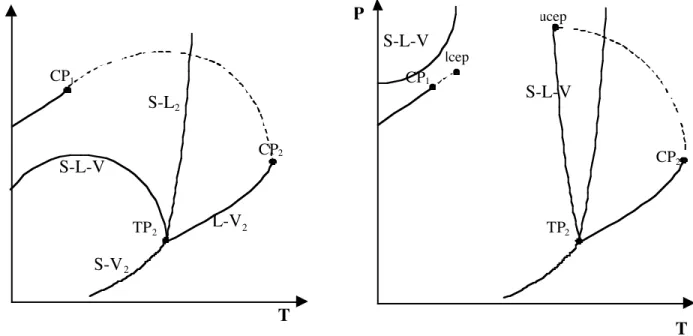
Two main types of diagrams P, T can be encountered:

In these diagrams, subscript 1 and 2 refer to the fluid and the solid respectively.

In the simplest case on the left diagram in figure 6, there is a continuous critical curve linking the two critical points of each component. A curve of coexistence of three phases (S-L-V) also appears. The shape of this curve shows that the melting point of the solid (the temperature at which a liquid phase appears) may decrease while the pressure is increasing. This phenomenon is known as the melting point depression. It corresponds to a dissolution of the light component into the solid leading to an easier fusion.

CP1 TP2 P S-L-V T CP2 CP1 TP2 P T CP2 lcep ucep S-L-V S-L-V S-L2 S-V2 L-V₂

This diagram represents a case where the fluid and the solid are "similar" in terms of molecular size and structure. It is seldom the case in industrial applications.

The more common case when there is a very different structure between the fluid (very often CO2) and the solid (very often a much bigger molecule with polarity) is represented on the

right-hand side diagram of figure 6. In this figure, the critical curve is no longer continuous. In the same way, the SLV curve has also split into two separate curves.

Two remarkable points appear: the lcep (lower critical end point) and the ucep (upper critical end point). Between these two points appears a “temperature window” of solubility in which whatever the pressure, there are only coexistence of a solid phase and a vapour phase with some heavy component dissolved.

How to use these diagrams: depending on the T,P operating conditions, several cases from a single monophase to a three-phase system can be encountered [31]. It is the P,y2 or T,y2 diagrams

which can give the exact configuration. II.5. Ternary systems

In many industrial applications a third component is involved. It may be a co-solvent which is able to enhance the solubility of a solute in the SCF. In particle design, the RESS process might be concerned. It may also be a solvent of the solute, the solution being then used in a process where the SCF is used as an anti-solvent (SAS process). Pöhler & Kiran [32, 33] have investigated the volumetric properties of CO2 with a cosolvent. The mixture composition may

become an additional parameter for an improved control of the process involved.

The co-solvent effect:

A co-solvent is a small polar molecule (light alcohol, acetone,..) which is added at low concentration in a supercritical fluid to modify its solvent power [34, 35]. The effect on solubility of some molecules may be tremendously affected. It is not rare to increase the solubility 100-fold with a few molar percent of a co-solvent.

A co-solvent changes the fluid density and its P,V,T properties. In addition, it can creates molecular specific interactions with the solute: hydrogen bonds, dipole interactions... Dobbs et al. [32, 33] studied the influence of polar and non-polar solvents. They showed that a polar co-solvent which can create hydrogen bonds with a solute increase the solubility in a non-polar supercritical solvent like CO2.

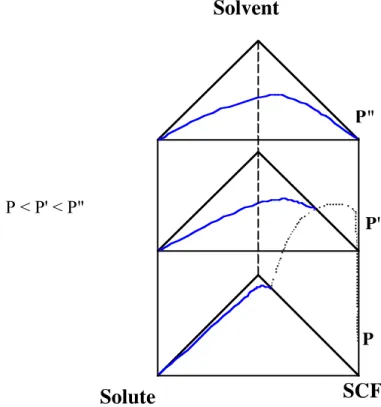
Phase diagrams:

are mainly used. To take into account the pressure variation the diagrams can be packed one on top on the others as shown on figure 7.

In this example the SCF and the solute are insoluble while the SCF is more and more soluble in the solvent as the pressure increases. The solvent and the solute are miscible at all pressures. The diagrams are represented for a temperature higher than the SCF critical temperature.

Each side of the prism is in fact a (P,y) diagram. On the side SCF-Solvent the dotted-line represents the pressure-composition behaviour of this binary mixture.

This example is a simple one with only a single-phase zone beyond the binodal curve and a two-phase zone under the binodal curve.

More complex diagrams can be encountered. Kikic et al. [38] gave an analysis of three-phase equilibria in binary and ternary systems for applications in particle generation processes.

II.6. Solubility measurements

The experimental techniques which can be developed for measuring solid solubilities in a SCF can be classified in two major groups [39]: synthetic methods and analytical methods.

P'

Solute

SCF

P"

P

Solvent

Figure 7. Phase diagram for a ternary mixture

Synthetic methods involve the determination of equilibrium without sampling. They normally require a static view cell of which the volume can be varied by any adapted system. It is the visual determination of the appearance or disappearance of a phase (bubble, dew) which gives the experimental data points. Once loaded with known amounts of the mixture to be studied a variation of temperature and cell volume allows the scanning of the P,T diagram.

In analytical methods, the compositions of the phases in equilibrium are obtained by analysis after sampling. These methods are the most widely used for determining solid-fluid equilibrium.

Among them there are the static and the phase-circulation methods. In the static methods, the solid is put in contact with the fluid and the mixture is allowed to attain an equilibrium state in appropriately stirred conditions. In these methods the difficulty is to get a sample without disturbing the equilibrium in order to have a good relevance of the analysis.

In the phase-circulation methods, a known quantity of fluid is allowed to re-circulate through a column in which the solute has been disposed, providing the agitation necessary to achieve thermodynamic equilibrium.

Finally, there are dynamic open-flow methods where the fluid passes through a bed of the solid. The fluid flow (which determines the contact time), the geometry of the equilibrium cell, determine whether or not the residence time is long enough to reach the equilibrium.

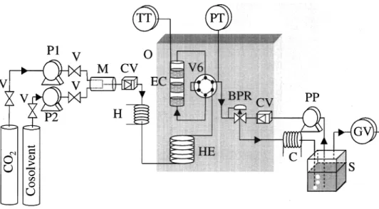
An example of such device is given on the figure 8. This apparatus was designed and built by the phase equilibria research team in the Ecole des Mines de Paris at Fontainebleau, France. It is based on a dynamic analytical method.

This apparatus was developed by Sauceau and co-workers to measure solid solubilities in pure CO2 and in CO2 plus a co-solvent [40]. Data obtained on naphthalene have been successfully

compared to those in the literature [2, 41]. A specific study on a pharmaceutical molecule was then performed [42, 43].

The equilibrium cell has been designed to achieve efficient stirring and efficient mass transfer in order to have the exiting supercritical mixture at thermodynamic equilibrium. A back pressure regulator (BPR) allows a constant pressure in the line. At the outlet, where the supercritical fluid is expanded to atmospheric pressure, the solid is allowed to crystallise and is immediately solubilised by a recovery liquid solvent stream. The apparatus is designed to avoid any dead volume and potential clogging by the solid, a problem encountered with most of the open circuit techniques used to measure solubilities in supercritical fluid.

The solubility of the solid in supercritical fluid is calculated from the total volume of gaseous solvent (extraction solvent) used and the concentration of solid in the recovery solute liquid phase. From these two measurements and knowing the total volume of the recovery solute liquid solvent, the solubility of the solid in the supercritical fluid can be calculated.

h ea t er , H , is u sed t o r a pidly h ea t t h e solven t t o t em per a t u r es a bove it s cr it ica l t em per a t u r e. Th e su -per cr it ica l flu id t h en en t er s a n oven (Spa m e), wh er e t h e solu bilit y cell is t h er m or egu la t ed. Th e oven ca n be u sed for t em per a t u r es u p t o 400 K, wit h t em per a t u r e r egu la -t ion wi-t h in 0.1 K. Beca u se of -t h e -t h er m a l in er -t ia of -t h e equ ilibr iu m cell, it s in t er n a l t em per a t u r e is fou n d t o be st a ble t o wit h in 0.05 K. A h ea t exch a n ger , H E , con -t a in ed in -t h e oven , is u sed -t o se-t -t h e -t em per a -t u r e of -t h e solven t a t t h e desir ed level (t em per a t u r e of t h e r equ ir ed solu bilit y m ea su r em en t ) befor e it en t er s t h e solu bilit y cell. H E con sist s of a br a ss cylin der a r ou n d wh ich is wou n d t h e st a in less st eel solven t cir cu it . Th e cylin der a n d t u bin g a r e cover ed wit h a br a ss r a dia t or . Down -st r ea m of t h e h ea t exch a n ger , a six-wa y, t wo-posit ion h igh -pr essu r e Va lco va lve is loca t ed in t h e cir cu it t o eit h er dir ect t h e su per cr it ica l flu id t o t h e cell or bypa ss it . Th is pr ovides a m ea n s for r em ovin g even t u a l solid deposit s fr om t h e lin e. Cylin dr ica l in sh a pe, t h e cell E C conta ins three compa rtments pla ced one a bove the other a n d fit t ed a t t h eir bot t om s wit h st a in less st eel sin t er ed disks a n d O r in gs. Th is is equ iva len t t o t h r ee differ en t cells con n ect ed in ser ies. Th e solid powder , for wh ich solu bilit y m ea su r em en t s a r e r equ ir ed, is pla ced in side t h e t h r ee com pa r t m en t s, wh ich h a ve a t ot a l volu m e of a bou t 5 cm3_{. Th e sin t er ed disks pr even t st r ippin g of t h e}

solid du r in g t h e exper im en t a n d a llow a sm a ll pr essu r e dr op, a dva n t a geou s for a t t a in in g sa t u r a t ion , wh ile a good disper sion of t h e su per cr it ica l solven t is a ch ieved. E C wit h st a n ds pr essu r es u p t o 50 MP a a t t em per a t u r es u p t o 400 K. Th e cell ca p is sea led in t h e bot t om pa r t u sin g a silicon e O r in g. Th e t wo pa r t s (ca p a n d bot t om ) a r e pr essed a ga in st ea ch ot h er wit h a fa st -con n ect in g m ech a n ica l device. Th e pr essu r e of t h e su per cr it ica l

473 K a n d 70 MP a . At t h e ou t let of t h e BP R, t h e pr essu r e is r edu ced t o a bou t a t m osph er ic pr essu r e, a n d t h en a r ecover in g liqu id solven t (a su fficien t ly good solven t a t a t m osph er ic pr essu r e t o r ecover a ll of t h e solu t e) st r ea m is u sed t o get t h e solu t e in liqu id st a t e for collect ion . Wit h ou t t h is solven t , t h e solu t e wou ld pr ecipit a t e du r in g t h e pr essu r e dr op, a n d t h is wou ld lea d t o pot en t ia l cloggin g. F in a lly, a sepa r a t or S is u sed t o ven t t h e ga s a n d collect t h e solven t ph a se. At t h e en d of ea ch exper im en t a l r u n , t h e liqu id solven t lin e is wa sh ed wit h fr esh solven t t o r ecover a ll of t h e solu t e. Th e t ot a l volu m e of ga seou s CO2 (ext r a ct ion solven t ), V1, is m ea su r ed by m ea n s of a volu m et er GV, a n d t h e con cen t r a t ion of solid in t h e solu t e r ecover in g liqu id ph a se C₂L is m ea su r ed by ga s or liqu id ch r om a t ogr a -ph y. Wit h t h ese t wo da t a a n d t h e t ot a l volu m e of t h e solu t e r ecover in g liqu id solven t , VL, det er m in ed, t h e

solu bilit y, y2, of t h e solid in su per cr it ica l flu id is

ca lcu la t ed by

wh er e

a n d

F ig u re 1. F low dia gr a m of t h e a ppa r a t u s.

y2) n₂

∑

4610 In d. E n g. Ch em . Res., Vol. 39, No. 12, 2000

III. PARTICLE GENERATION: LIMITATIONS OF TRADITIONAL

PROCESSES AND INTERESTS IN USING SFC-BASED

TECHNOLOGIES

The use of materials as finely divided powder is ubiquitous in industry. Whatever the domain involved: mineral industry, fine chemistry, cosmetics, agro-food industry, paints, pharmaceuticals, detergents, ... powders are largely used.

Generation of fine particles can be achieved by two main routes:

• size reduction: crushing, grinding, milling, comminution, micronisation

• crystallisation: precipitation, atomisation, crystallisation by evaporation, cooling or variation in ionic strength

III.1. Size reduction

Because of their relative simplicity the processes using the first route are still extremely used in industry.

However, they have inherent drawbacks which may hinder or even prevent their use: • Low energetic yield

• Pollution by the grinding medium

• Limited control on particle size (generation of undesired dust) • No control on particle shape

• Broad particle size distribution

• Not usable with thermolabile products or hazardous chemicals

• A low limit in mean particle size of a few micrometers beyond which it is extremely difficult to go

• In some specific applications there is the need of the use of an adjuvant • At least one step of sieving is compulsory to complete the process

III.2. Crystallisation

The second route uses the generation of a solid phase from a fluid phase. The most classical processes using this route are:

• Spray-drying, atomisation: the liquid medium (very often water) is evaporated by exposure for a short time at high temperature yielding a solid residue previously solubilised in the medium

• Precipitation: a chemical reaction involving two (or more) reactants leads to the formation of a solid phase insoluble in the liquid

• Crystallisation: by tuning either the temperature, the pH, the ionic strength or by evaporating the solvent, nuclei of solid particles are formed and grow, finally leading to a powder.

As in the first route this second type of processes share several disadvantages: • no control of crystal polymorphism

• residual solvent

• need for an additional drying step

All these processes are performed at atmospheric pressure, which is very seldom used as a variable.

III.3. Supercritical fluid technology

Supercritical fluid technology appears to be a third route for particle generation [44, 45]. Most of the drawbacks of the two previous routes are avoided and in addition some products cannot be micronized by the classical methods. Supercritical processes give micro or even nanoparticles with narrow size distribution and can also be used to manufacture microencapsulation or surface coating of an active substance particle with a polymer.

One of the main feature of supercritical fluid technology is the use of pressure as a very useful and practical operating parameter. Their use as a medium from which a solid phase can be obtained has been known for a long time [14]. However its only very recently (about twenty years ago) that scientific reports were published in which those properties were developed for particle generation.

IV. THE RESS PROCESS

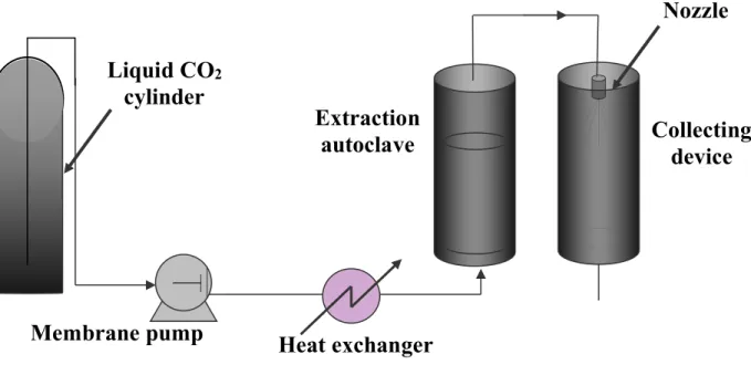
IV.1. Principle of the process

Figure 9. The RESS process: schematic flow diagram

RESS stands for Rapid Expansion of Supercritical Solutions and is sometimes called spray crystallisation [46].

Its principle is very simple:

As shown in the introduction section a SCF may exhibit good solvent capacity for solid compounds. Moreover, this solvent power is dependent on the fluid density, which can be varied by modifying temperature and pressure ("a SCF is dense and compressible" in other words it can be a good or a poor solvent depending on the operating conditions).

Therefore a solid dissolved in a SCF can be crystallised from the homogeneous supercritical solution -P and T are chosen to give a monophase mixture- provided the density is low enough. The easiest way to provoke a drop in density is to force the fluid to pass through a hole or a capillary or a nozzle in which an adiabatic expansion can be achieved. Nozzle diameter must be small enough to allow a large depressurisation. Typically it is of a few decades of micrometers. Downstream from the nozzle, the fluid is generally in the gaseous state with a very poor solvating power. Figure 9 gives a schematic view of a device for RESS particle production.

Liquid CO

cylinder

Heat exchanger

Membrane pump

Collecting

device

Extraction

autoclave

Nozzle

IV.2. Optimisation of the RESS process

First of all, it is necessary to have the best possible understanding of what happens upstream from the nozzle that is to say during the extraction step. Therefore, it is important either to collect data from the literature when they exist, or to perform experiments or modelling, about the solute solubility in the SCF. Chapter 2 gives a brief overview of the measurement and the modelling of the solubility of a solid in a SCF.

The key parameters of this extraction step are obviously the operating T and P. The flow rate of the fluid may also play an important role since a thermodynamic equilibrium may or may not be reached in the extraction autoclave. In fact, the kinetics of the dissolution must not be neglected and diffusional limitations can occur. Additional problems may be encountered when the solid to be extracted is not a pure component. Fractionation of the load can lead to a variation in the composition of the particles upon depressurisation.

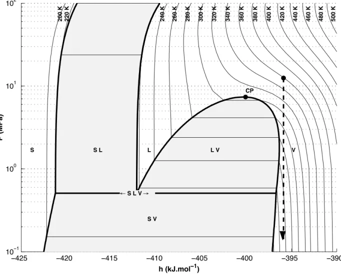
Figure 10. RESS expansion in the pressure-enthalpy diagram for pure CO2

−425 −420 −415 −410 −405 −400 −395 −390 10−1 100 101 102 200 K 220 K 240 K 260 K 280 K 300 K 320 K 340 K 360 K 380 K 400 K 420 K 440 K 460 K 480 K 500 K h (kJ.mol−1) P (MPa) ← S L V → S S L L L V V S V CP

To understand what will happen during fluid expansion, a Mollier diagram (pressure P vs. molar enthalpy h) is very useful [47]. An acceptable assumption is to consider that the depressurisation is an iso-enthalpic process (in fact there is a variation of kinetic energy of the fluid, which should be taken into account). Therefore, the expansion step will be a vertical line on this diagram.

Such a drop in pressure implies an important decrease in temperature as shown on figure 10 which is the Mollier diagram for pure CO2.

In the example shown on this figure, the starting point as well as the arrival point, are chosen to be in the single-phase zone of the diagram. However, to ensure such conditions, the temperature before expansion must be rather high which may be incompatible with the solute to be extracted. A lower pre-expansion temperature may lead to a condensation or freezing of the SCF (the triple point of CO2 is at 5.2 bars).

Some authors have pointed out the fact that to compensate this drop in temperature, the nozzle can be heated [48]. The potential problems are clogging due to the solute crystallisation and the possible appearance of a liquid and/or a solid phase of the solvent.

In order to avoid these problems, several possibilities exist: a proper geometry of the nozzle (length, diameter, ratio of one to the other,...) can prevent any plugging, while an adequate choice of the values of T and P (as shown on the diagram) may allow only a single fluid phase and a solid phase. In particular, the pre-expansion temperature as already noted but also the post-expansion pressure are of the utmost importance.

Nevertheless, this latter solution is not always practicable, particularly with thermosensitive molecules. In such cases a heated nozzle or a heating device just upstream from the nozzle can be very useful. To determine the thermodynamic route of the depressurisation, it is necessary to calculate the heat transfer from the nozzle to the fluid.

Nucleation of the solute occurs during the sudden expansion of the solution and is due to the mechanical perturbation, which propagates at the speed of sound leading to very uniform conditions [49] and therefore to a very narrow particle size distribution.

Indeed, the expansion time depends not only on the speed of sound (which varies with the operating conditions and the nature of the fluid) but also on the length of the capillary nozzle. However, an approximation between 10-4 _{to 10}-6 _{second has been proposed [50].}

It is during this very short period of time that solubility falls by several orders of magnitude leading to large supersaturation ratios. This ratio is defined as the concentration of the solute over the solubility (the concentration at saturation).

Eq. (21)

S =

c

The driving force of the nucleation process is the difference between the chemical potential of the solid in both phases (fluid and solid) which is related to the activity of the solute in the solution and at equilibrium [51]. A simpler way to express this is to say that the supersaturation drives the nucleation.

This supersaturation comes from the drop in density which is very large especially near the critical point. The value of the enhancement factor (see & 2.1) which can be as high as 105 _{or 10}6_,

can give an idea of the large supersaturation ratios obtained, provided the fluid after expansion can be considered to be an ideal gas. This is the case when the expansion pressure is close to atmospheric pressure.

However, the expansion, may not be complete and can be controlled. It may be advantageous to limit the depressurisation and to let a pressure of a few tens of bars. This will diminish the supersaturation ratio but the recycling of the fluid might be facilitated. In fact relatively small changes in pressure may cause a dramatic fall in density and therefore in solubility. Again, the h,P diagram shown in figure 10 is of great help to determine which conditions can be used.

The most obvious drawback of RESS is the lack of solubility of several families of molecules in the CO2. To overcome this problem one way is to change the supercritical fluid. However, this

is seldom possible since the few other candidate molecules (N2O, light hydrocarbons,...) are

much more hazardous than is CO2 [52].

Another possibility is to use the RESS process with a co-solvent [53] being previously dissolved in the CO2. In this case the advantage of not using any chemical solvent is lost but it

might be interesting to use a co-solvent using such low-toxicity solvents like acetone or ethanol.

The phase diagrams (h, P or P, T) of the binary mixture is different from the pure component diagram. As an example, the P, T diagram for the mixture (95 % CO2 - 5% Ethanol) shows that

the two-phase envelope is considerably enlarged by the addition of 5 % co-solvent (figure 11). This has to be taken into account when determining the operating conditions.

Chang and Randolph [54] showed that addition of up to 1.5 % mole fraction of toluene in supercritical ethylene enhances b-carotene solubility while particles obtained trough expansion remained unchanged. The maximum mole fraction was determined to maintain a single phase fluid after depressurisation.

The choice of the proper co-solvent is not trivial and the affinity two-by-two supercritical fluid, co-solvent and solute are to be considered. A mixture of co-solvents may also be used [55].

Moreover, it is not possible to predict the co-solvent effect from the solubility of the solute in the liquid co-solvent. Therefore, solubility measurements of the solid in the mixture SCF-co-solvent are highly recommended [44, 56].

Mole fractions: CO2=95% and Ethanol=5% (Calculation: PR EOS)

Figure 11. P,T diagram of a CO2-Ethanol mixture

IV.3. Particle size and morphology: towards a modelling of the process

The particles obtained by this route are expected to be small with a narrow particle size distribution (PSD).

The rate of nucleation as well as the size of nuclei is inversely proportional to the square of Ln S. Very high values of S will therefore give very large number of small nuclei.

One possible way to control particle size is therefore to adapt the supersaturation by varying the drop in pressure through the nozzle. Alessi et al. [57] have shown that an increase in the pressure of the expansion vessel or a decrease in the pressure upstream the nozzle led to an

mean particle size is much larger (most articles claim particles ranging from several hundreds of nm to a few µm) than those predicted by the theory. Debenedetti [59] gave a critical nucleus size of 20 nm for phenanthrene in SC-CO2. Nevertheless, submicronic particles can be obtained [60].

By modelling the evolution of pressure, temperature and density along a capillary nozzle, Debenedetti et al. [61] have evidenced the role of density in a capillary nozzle on particle size and morphology. Ksibi et al. [62] made a numerical simulation of the RESS process in which solute nucleation is taken into account in addition to the jet hydrodynamics influenced by the nozzle geometry.

Working with polymers in CHF2Cl, Lele & Shine [63] also found that the morphology

changes with the fluid density at the nozzle entrance. The same authors [64] could correlate the morphology obtained, fine particles or fibres, with the time-scale available for phase separation. It is noticeable that for polymers the precipitation occurs from a polymer liquid rich phase after a liquid-liquid phase separation. Large fibres were obtained when phase separation had occurred early, upstream the nozzle, while fine (0.2 to 0.6 µm) particles were produced for a late, in the nozzle, phase separation.

More recently, Helfgen et al. [65] developed a numerical model to predict particle formation. Using CO2 and CHF3 as solvents they made particles of cholesterol, griseofulvin and benzoic

acid. They showed that the nucleation occurred in the supersonic free jet and that particle growth was mainly due to coagulation.

IV.4. Applications of the RESS

There are numerous published examples of particles produced by RESS.

There are some reports with inorganic compounds, mainly not with CO2 (such compounds

exhibit too low a solubility in CO2)but other solvents like pentane or water. In the domain of

ceramics processing, Matson et al. [66, 67] worked on ceramics and produced powders and fibres from silica and polycarbosilane. To intimately blend different ceramic materials a possible process is to dissolve them in supercritical water and to expand the solution to form ultrafine powders. These powders are then sintered and this next operation can be greatly facilitated by finely divided and ultra-pure powders.

Among the papers reported with other supercritical solvents, Sun et al. [68] made nanoscale lead sulphide (PbS is a semiconductor) using a RESS process modified in two ways. The expansion was done in a liquid solution and a reaction occurred, one reactant being dissolved in the SCF and the other in the liquid receiving solution. The solvents used were ammonia, methanol and acetone.

It is however the domain of organic molecules which have been the most extensively studied. There are a few examples of applications in the agro-food industry:

• Cocoa butter which crystals present several polymorphs [69] is a good candidate to be treated by RESS [70]

• b-carotene, a vitamin precursor which presents a rather good solubility in supercritical CO2

[71, 72], nitrous oxide [4] and ethane [73], will probably deserve to be studied in the goal to produce particles [54].

However, most of the foodstuffs are not expensive enough to allow a crystallisation by means of supercritical technology.

Due to their high added value, it is the pharmaceuticals, which are by far the most studied. The use of RESS for producing drug controlled release systems (with a polymer) has also been widely studied.

Several reviews have already listed most of these works [48, 49, 74]. Among the pharmaceuticals one can cite (from supercritical CO2 instead otherwise specified):

• lovastatin, a hypocholesterol drug [75, 76], • b-estradiol, a steroid [15],

• salicylic acid, an antalgic [77], • caffeine, theophylline [78], • cholesterol [65, 79],

• phenacetin, an analgesic [80],

• hormones: progesterone, testosterone [48], • ibuprofene, an anti-inflammatory drug [81], • stigmasterol [82],

• griseofulvin, an antifungal drug, obtained from supercritical CHF3 [83],

• carmabazepine, an anticonvulsant [84],

However it is clear that a lot of work done in the research laboratories of pharmaceutical companies have never been published.

Knutson et al. [74] reviewed the use of the RESS process for producing polymeric microspheres containing active substances. These devices are aimed for controlled drug delivery and are very often made of an active drug coated by or encapsulated in a biocompatible polymer. The most used polymers are the poly-lactic acids (PLA) and poly-glycolic acids (PGA) which are known for their good compatibility with the human body.

The drug and the polymer must be dissolved in the fluid (generally CO2). They can be

dissolved in the same vessel or independently and both streams are joined before entering the nozzle. Because of the poor CO2 solubility of most polymers, co-solvents such as

fluorohalocarbons have been used [85]. However, their toxicity as well as their negative impact on the environment reduce the interest for such a process.

Lovastatin, has been crystallised as needles embedded in microspheres of DL-PLA [74]. IV.5. Conclusion and perspectives for RESS

RESS remains interesting because of its simplicity of use. It has proven to be usable with all kind of molecules and particularly with active pharmaceutical drugs. It can also be used with polymers to give encapsulated particles for control drug delivery.

The conditions gathered in a RESS process exhibit several advantages due to the huge supersaturation ratios and the fact that the solvent after expansion returns to a gaseous state:

• Particles are very fine • Particles are monodisperse • The fluid can be recycled

• There is no contamination or residual solvent • Thermolabile molecules can be processed

• Chemical or shock sensitive molecules can be processed • Control of polymorphism is sometimes possible[84].

In spite of a very large numbers of publications on this process, most authors agree that RESS is very often limited by the solubility of the solute to be crystallised. This explains why processes using a supercritical fluid as an anti-solvent have been so widely developed in recent years (see chapter 5). In addition, a lot of work on modelling the nucleation and growth of the crystals in the jet remains to be done. Most of the reports show that particle size and morphology are generally not well controlled and each particular case needs a specific study. The influence of nozzle geometry probably deserves much more work.

However, when facing the problem of getting a very fine crystalline powder, RESS remains the first process to test. A low solubility can in some instances be accepted or overcome. Appropriate tuning of the fluid density and the use of an adequate co-solvent are two powerful tools which use may completely change the fate of the industrial use of RESS for a specific molecule.

An additional advantage, on an industrial point of view, lies in the fact that the principle of RESS have been described for more than one century ago. That means that no patent can be filed on the particle generation itself.

V.

THE SAS PROCESS AND RELATED TECHNOLOGIES

V.1. Principle of the process

Figure 12. The SAS process: schematic flow diagram

When the solute is not soluble enough in a supercritical fluid, this can be used as an anti-solvent.

This type of process is particularly recommended with molecules such as sugars, proteins, polymers, metallic oxides and polymers that are known for their very poor solubility in SC CO2.

The general acronym for this family of processes is SAS for Supercritical Anti Solvent. The rationale of the process is as follows:

In addition to the substance to be produced as a powder and the SCF, a third component, very often an organic solvent has to be used. This solvent is chosen for being a good solvent of the component to be micronised and ideally, it should meet three different requirements:

- it must solubilise the solute in relatively large amounts

- it must have good compatibility with the anti-solvent. It is even better if it is completely

Pump

Liquid

CO

cylinder

Mixing device

Collecting basket

Solution vessel

Heat exchanger

When both the organic solution and the anti-solvent are contacted, the antisolvent dissolves in the organic phase decreasing the density, the solvent power and therefore the solubility of the solute. At the same time the solvent evaporates in the supercritical phase increasing the solute concentration. It is this mass transfer in both directions which accounts for the rapid supersaturation of the solute and therefore the nucleation of crystals.

Several ways of achieving a SAS process can be encountered:

• Figure 12 gives a schematic view of a SAS device in which both streams are contacted at the nozzle. This operating method has been referred to as the SEDS process, for Solution Enhanced Dispersion by Supercritical Fluids [86]. It is a continuous process except for the particle collection which has to be done batchwise. The solvent can be collected in separators while the antisolvent can be recycled by compression, heating and re-injection. Washing of the expansion vessel with pure SCF is recommended before particle collection. Ruchatz et al. [87], have demonstrated the importance of process parameters on the solvent residues concentration.

Several other possibilities exist:

• For instance the SCF can be injected in the solution in a closed vessel (batch mode) which is known as GAS process for Gaseous Anti Solvent. In this case the rate of addition of the SCF is obviously an important parameter. The SCF provokes an expansion of the solution which in turn gives supersaturation and particle formation. The vessel has to be returned to atmospheric pressure to collect the particles The solvent must therefore be eliminated by flow supercritical fluid throughout the vessel in order to "dry" the particles. An appearance of a liquid phase rich in organic solvent must be avoided in order not to solubilise the solute again. This batch mode has several drawbacks: the pressure increases continuously during operation meaning that the supersaturation is not controlled, which leads to wide particle distribution. Moreover, it is not really suited to industrial applications.

• The organic solution can be sprayed in a vessel in which supercritical fluid is flowing. The dissolution of the SCF in the solution droplets provokes the particle generation, which can be collected afterwards in the vessel while the mixture SCF-solvent can be sent to a separator. This process is called ASES (for Aerosol Extraction Solvent System).

• Such a process in batch mode, where the solution is introduced into a closed vessel containing the dense compressed anti-solvent [88] has been given the name PCA (for Precipitation with Compressed Antisolvent).

V.2. Optimisation of the SAS process

Several parameters have an influence on the size and the morphology of the obtained particles. As with the RESS process the operating T and P upstream and downstream from the nozzle are obviously key-parameters. The role of the nozzle is to favour droplet formation which is rather different from the RESS case in which the main role of the nozzle is to provoke a huge drop in pressure. Nozzle geometry is also an important parameter in controlling the process. In addition, the concentration of the solute in the solution and the relative flow rates of the solution and the anti-solvent are also to be taken into account.

The volumetric expansion of the organic solvent due to the dissolution of the anti-solvent has been recognised as an important parameter [89, 90]. Most of the former papers described SAS in batch mode and therefore the main phenomenon was the volumetric expansion of the organic solution upon injection of a compressed SCF.

This expansion is defined by the following equation:

Eq. (22)

V is the volume of the liquid expanded phase while V0 is the volume of the pure solvent

before the anti-solvent injection.

Using a view cell it has been possible to directly measure the volumetric expansion. As an example, figure 13 shows the volumetric expansion of a classical organic solvent, DMSO, in CO2. The volume of the liquid phase increases with pressure. However, for a given pressure the

volume expansion is less pronounced as the temperature increases. Warwick et al. [91] showed such an expansion with another solvent, DMF, versus the mole fraction of CO2. It was noticed

that all the isotherms overlap in a single curve which have the same shape of those presented in figure 13. Therefore, the volume expansion for a given solvent depends only on the mole fraction of both constituents.

The volume expansion can be predicted by using an equation of state with quadratic mixing rules (see & 2.2). Reverchon [92] reviewed the studies in which several authors have measured this expansion depending on the operating conditions and on the nature of the solvent. These observations are of the utmost importance for the batch mode processes where the particle are produced from a liquid phase rich in solvent.

ΔV =

V (P, T) - V

V

De la Fuente et al. [93] defined the volumic expansion from the molar volumes and they showed on the mixtures CO2-toluene-phenanthrene and CO2-toluene-naphtalene that the

minimum of volumic expansion corresponds to the solid crystallisation.

Figure 13 (from Reverchon, [92]). Volumetric expansion of DMSO in CO2

From an industrial point of view, it is the semi-continuous mode where there is a co-injection of the supercritical anti-solvent and the liquid solution which appears to be the most promising.

The expansion curves are therefore less pertinent since the phenomena involved are rather different. The particles are formed from the drops of the solution which collide into the fluid phase. As the antisolvent flow rate is generally much higher than those of the solution, one can use the P,h diagram to see how many phases are present at the equilibrium.

An example has been given in figure 11 with the diagram of a 95 % CO2-5% Ethanol mixture.

This may correspond to a practical ratio of the anti-solvent over the solution of about 20. This diagram shows the two-phase envelope which is to be avoided in order not to have a liquid phase in the expansion chamber. Such a liquid phase might re-solubilise the particles formed.

V.3. Particle formation mechanisms

In semi-continuous processes which are those most studied today because of their potential industrial applications, the mass-transfer and nucleation occur at the surface of solution droplets

200 400 Volumetric expansion (%) 100 50 P (bar) 313 K 308 K 303 K

in a continuous flow of antisolvent. It is therefore necessary to understand the fate of these droplets. There is a competition between two phenomena which occur simultaneously:

• the anti-solvent effect i.e. the dissolution of the anti-solvent into the solution. The consequence is the swelling of the solution droplets.

• the evaporation of the solvent into the anti-solvent. The consequence is the shrinking of the solution droplets.

A key-question must therefore be addressed:

Do the droplets of solvent in a flow of antisolvent swell or shrink?

Shekunov et al. [94] showed results obtained with optical methods, image analysis, laser interferometry and PIV. They showed that droplets of ethanol in a turbulent flow of supercritical CO2 do not swell as expected but on the contrary seem to retract as long as the ethanol dissolves

("evaporates") in the CO2. Depending on the pressure (below or above the critical mixture point)

the behaviour of the droplet changes:

At low pressures (below the mixture critical pressure) the droplets of ethanol decrease regularly. Nucleation and growth of crystals occur at the droplet interface leading to agglomerated particles.

At higher pressures, a liquid ethanol jet appears from each droplet. Nucleation occurs within the shrinking ethanol-rich droplets and the mixing regime has a great importance. No swelling has been observed whatever the operating conditions.

Reverchon [92] observed that the particle morphology is linked with the expansion volume DV. Interpretating the results from different series of batchwise experiments, this author assumed an expansion of liquid droplets in all cases.

Low DV led to agglomerated particles. Obtained in batch mode, these particles were obtained from a crystallisation in the liquid phase.

Intermediate values for DV gave particles in the shape of hollow spheres called "balloons". The proposed mechanism is a fast expansion of the droplets.

Finally, at the highest values for DV, the smallest particles with a narrow particle size distribution were obtained. Balloon disintegration was proposed for the involved mechanism. However, a crystallisation from fast-shrinking droplets cannot be excluded.

In addition, some growth phenomena such as coalescence can also greatly modify the morphology of the final powder.

V.4. Modelling the SAS process

Phase equilibria calculations are at the basis of tentative for modelling SAS. However, when using a semi-continuous process, the data from fluid phase equilibria analysis are not sufficient. Fluid dynamics and crystallisation must also be taken into account. Crystallisation is by