HAL Id: hal-02884657
https://hal.archives-ouvertes.fr/hal-02884657
Submitted on 15 Jul 2020
HAL is a multi-disciplinary open access
archive for the deposit and dissemination of
sci-entific research documents, whether they are
pub-lished or not. The documents may come from
teaching and research institutions in France or
abroad, or from public or private research centers.
L’archive ouverte pluridisciplinaire HAL, est
destinée au dépôt et à la diffusion de documents
scientifiques de niveau recherche, publiés ou non,
émanant des établissements d’enseignement et de
recherche français ou étrangers, des laboratoires
publics ou privés.
targeted maximum likelihood estimator for causal
inference with different covariates sets: a comparative
simulation study
Arthur Chatton, Florent Le Borgne, Clémence Leyrat, Florence Gillaizeau,
Chloé Rousseau, Laetitia Barbin, David Laplaud, Maxime Léger, Bruno
Giraudeau, Yohann Foucher
To cite this version:
Arthur Chatton, Florent Le Borgne, Clémence Leyrat, Florence Gillaizeau, Chloé Rousseau, et al..
G-computation, propensity score-based methods, and targeted maximum likelihood estimator for causal
inference with different covariates sets: a comparative simulation study. Scientific Reports, Nature
Publishing Group, 2020, 10 (1), pp.9219. �10.1038/s41598-020-65917-x�. �hal-02884657�
G-computation, propensity
score-based methods, and targeted
maximum likelihood estimator
for causal inference with different
covariates sets: a comparative
simulation study
Arthur chatton
1,2, florent Le Borgne
1,2, clémence Leyrat
1,3, florence Gillaizeau
1,4,
chloé Rousseau
1,4,5, Laetitia Barbin
4, David Laplaud
4,6, Maxime Léger
1,7, Bruno Giraudeau
1,8& Yohann foucher
1,4✉
controlling for confounding bias is crucial in causal inference. Distinct methods are currently employed to mitigate the effects of confounding bias. Each requires the introduction of a set of covariates, which remains difficult to choose, especially regarding the different methods. We conduct a simulation study to compare the relative performance results obtained by using four different sets of covariates (those causing the outcome, those causing the treatment allocation, those causing both the outcome and the treatment allocation, and all the covariates) and four methods: g-computation, inverse probability of treatment weighting, full matching and targeted maximum likelihood estimator. our simulations are in the context of a binary treatment, a binary outcome and baseline confounders. the simulations suggest that considering all the covariates causing the outcome led to the lowest bias and variance, particularly for g-computation. The consideration of all the covariates did not decrease the bias but significantly reduced the power. We apply these methods to two real-world examples that have clinical relevance, thereby illustrating the real-world importance of using these methods. We propose an R package RISCA to encourage the use of g-computation in causal inference.
The randomised controlled trial (RCT) remains the primary design for evaluating the marginal (population average) causal effect of a treatment, i.e., the average treatment effect between two hypothetical worlds where: i) everyone is treated and ii) everyone is untreated1. Indeed, a well-designed RCT with a sufficient sample size
ensures the baseline comparability between groups, thus allowing the estimation of a marginal causal effect. Nevertheless, it is well established that RCT is performed under optimal circumstances (e.g., over-representation of treatment-adherent patients, low frequency of morbidity), which may be different from real-life practices2.
Observational studies have the advantage of limiting the issue of external validity, but treated and untreated patients are often non-comparable, leading to a high risk of confounding bias.
To reduce such confounding bias, the vast majority of observational studies have been based on multivariable models (mainly linear, logistic, or Cox models), allowing for the direct estimation of conditional (subject-specific) effects, i.e., the average effect across sub-populations of subjects who share the same characteristics. Several
1INSERM UMR 1246 - SPHERE, Université de Nantes, Université de Tours, Nantes, France. 2A2COM-IDBC, Pacé, France. 3Department of Medical Statistics & Cancer Survival Group, London School of Hygiene and Tropical Medicine, London, UK. 4Centre Hospitalier Universitaire de Nantes, Nantes, France. 5INSERM CIC1414, CHU Rennes, Rennes, France. 6Centre de Recherche en Transplantation et Immunologie INSERM UMR1064, Université de Nantes, Nantes, France. 7Département d’Anesthésie-Réanimation, Centre Hospitalier Universitaire d’Angers, Angers, France. 8INSERM CIC1415, CHRU de Tours, Tours, France. ✉e-mail: [email protected]
methods have been proposed to estimate marginal causal effects in observational studies, amongst which pro-pensity score (PS)-based methods are increasingly used in epidemiology and medical research3.
Propensity score-based methods make use of the PS in four different ways to account for confounding, namely matching, stratification, conditional adjustment4 and inverse probability of treatment weighting (IPTW)5.
Stratification and conditional adjustment on PS are associated with the highest bias6–8, because the two methods
estimate the conditional treatment effect rather than the marginal causal effect. Matching on PS remains the most common approach with a usage rate of 83.8% in 303 surgical studies using PS-based methods9 and 68.9% in 296
medical studies (without restriction regarding the field) also using PS-methods10. The IPTW appears to be less
biased and associated with a lower variance than matching in several studies8,11–14. Nevertheless, in particular
settings, full matching (FM) was associated with lower mean square error (MSE) in other studies15–17.
Multivariable models, even non-linear ones, can also be used to indirectly estimate the marginal causal effect with g-computation (GC)18. This method is also called the parametric g-formula1 or (g-)standardisation19 in
the literature. Snowden et al.20 and Wang et al.21 detailed the corresponding methodology for estimating the
average treatment (i.e., marginal causal) effect on the entire population (ATE) or only on the treated (ATT), respectively. The ATE is the average effect, at the population level, of moving an entire population from untreated to treated. The ATT is the average effect of treatment on those subjects who ultimately received the treatment22.
Furthermore, some authors23,24 have proposed combinations of GC and PS to improve the estimation of the
marginal causal effect. These methods are known as doubly robust estimators (DRE) because they require the specification of both the outcome (for GC) and treatment allocation (for PS) mechanisms to minimise the impact of model misspecification. Indeed, these estimators are consistent as long as either the outcome model or the treatment model is estimated correctly25.
Each of these methods carries out the adjustment in different ways, but all of these methods rely on the same condition: a correct specification of the PS or the outcome model1. In practice, a common issue is choosing the
set of covariates to include to obtain the best performance in terms of bias and precision. Three simulation stud-ies7,26,27 have investigated this issue for PS-based methods. They studied four sets of covariates: those causing the
outcome, those causing the treatment allocation, those are a common cause of both the treatment allocation and the outcome, and all the covariates. For the rest of this paper, we called these strategies the outcome set, the
treat-ment set, the common set and the entire set, respectively. These studies argued in favour of the outcome or
com-mon sets for PS-based methods, but it is not immediately clear that such works will generalise to other methods of causal inference. Brookhart et al.26 and Lefebvre et al.27 focused on count and continuous outcomes. Austin et al.7
investigated binary outcomes on matching, stratification and adjustment on PS. However, GC and DRE also require the correct specification of the outcome model with a potentially different set of covariates. Recent works have shown that efficiency losses can accompany the inclusion of unnecessary covariates28–31. De Luna et al.32 also
highlighted the variance inflation caused by the treatment set. In contrast, VanderWeele and Shpitser33 suggested
the inclusion of both the outcome and the treatment sets.
Before selecting the set of covariates, one needs to select the method to employ. Several studies have compared the performances of GC, PS-based methods and DRE in a point treatment study to estimate the ATE13,23,25,34–36.
Half of these studies investigated a binary outcome13,25,34. Only Colson et al.17 studied the ATT, but they focused
on a continuous outcome. Except in Neugebauer and van der Laan25, these studies only investigated the ATE (or
ATT) defined as a risk difference. The CONSORT recommended the presentation of both the absolute and the relative effect sizes for a binary outcome, “as neither the relative measure nor the absolute measure alone gives a
complete picture of the effect and its implications”37. None of these studies was interested in the set of covariates
necessary to obtain the best performance.
In our study, we sought to compare different sets of covariates to consider to estimate a marginal causal effect. Moreover, we compared GC, PS-based methods and DRE for both the ATE and ATT, either in terms of risk dif-ference or marginal causal OR. Three main types of outcome are used in epidemiology and medical research: con-tinuous, binary and time-to-event outcomes. We focused on a binary outcome because i) a continuous outcome is often appealing for linear regression where the two conditional and marginal causal effects are collapsible38, and
ii) time-to-event analyses present additional methodological difficulties, such as the time-dependant covariate distribution39. We also limit our study to a binary treatment, as in the current literature, and the extension to three
or more modalities is beyond the scope of our study.
The paper is structured as follows. In the next section, the methods are detailed. The third section presents the design and results of the simulations. In the fourth section, we consider two real data sets. Finally, we discuss our results in the last section.
Methods
Setting and notations.
Let A denote the binary treatment of interest ( =A 1 for treated patients and 0 oth-erwise), Y denote the binary outcome ( =Y 1 for events and 0 otherwise), and L denote a set of baseline covariates. Consider a sample of size n in which one can observe the realisations of these random variables: a, y, and l, respec-tively. Define π =a E P Y( ( =1 (do A=a L), )) or π =a E P Y( ( =1 (do A=a L A), ) =1) as the expectedpropor-tions of event if the entire (ATE) or the treated (ATT) populapropor-tions were treated (do A( =1)) or untreated (do A( =0)), respectively40. From these probabilities, the risk difference can be estimated as π∆ =π −π
1 0 and
the log of the marginal causal OR estimated as θ=logit( )/logit( )π1 π0, where logit(•) = log(•/(1 − •)). The
meth-ods described bellow allow for the estimation of both the ATE and the ATT effects.
Causal inference requires the three following assumptions, called identifiability conditions: i) The values of exposure under comparisons correspond to well-defined interventions that, in turn, correspond to the versions of treatment in the data. ii) The conditional probability of receiving every value of treatment, though not decided by the investigators, depends only on the measured covariates. iii) The conditional probability of receiving
every value of the treatment is greater than zero, i.e., is positive. These assumptions are known as consistency,
(conditional) exchangeability and positivity, respectively1. However, PS-based methods rely on treatment
alloca-tion modelling to obtain a pseudo-populaalloca-tion in which the confounders are balanced across treatment groups. Covariate balance can be checked by computing the standardised difference of the covariates included in the PS between the two treatment groups10. In contrast, GC relies on outcome modelling to predict hypothetical
outcomes for each subject under each treatment regimen. Note that one can ignore the lack of positivity if one is willing to rely on Q-model extrapolation1. As is the case for standard regression models, these methods also
require the assumptions of no interference, no measurement error and no model misspecification.
Weighting on the inverse of the propensity score.
Formally, the PS is =pi P A( i =1 )Li, i.e. the proba-bility that subject i ( =i 1,…,n) will be treated according to his or her characteristics Li at the time of the treatment allocation4. It is often estimated using a logistic regression. The IPTW makes it possible to reduce confounding bycorrecting the contribution of each subject i by a weight ωi. For ATE, Xu et al.41 defined
ω =i A P Ai ( i=1)/pi +(1−A P Ai) ( i =0)/(1−pi). The use of stabilised weights has been shown to produce a suitable estimate of the variance even when there are subjects with extremely large weights5,41. For ATT, Morgan and
Todd42 defined ω =A +(1−A p) /(1−p)
i i i i i. Based on ωi, the following weighted univariate logistic regression
can be fitted: logit{ (P Y=1 )}A =αˆ0+αˆ , resulting in π1A ˆ0=(1+exp(−αˆ0))−1, πˆ1=(1+exp(−αˆ0−αˆ1))−1,
and θˆ=αˆ1. To obtain var( ), we used a robust sandwich-type variance estimator ˆθ 5 with the R package sandwich43.
full Matching on the propensity score.
The FM minimises the average within-stratum differences in the PS between treated and untreated subjects16. Then, two weighting systems can be applied in each stratum, makingit possible to estimate either the ATE or the ATT unlike other matching methods which can only estimate the ATT44. If t and u denote the number of treated and untreated subjects in a given stratum, one can define the
weight for a subject i in this stratum as ω =i A P Ai ( =1)(t+u u)/ +(1−Ai)(1−P A( =1))(t+u t)/ for ATE and ω =i Ai+(1−A t ui) / for ATT16. In the latter case, the weights of untreated subjects are rescaled such that the sum of the untreated weights across all the matched sets is equal to the number of untreated subjects:
ωi=ωi× ∑nj=1(1−Aj)/∑nj=1ωj(1−Aj)45. From the resulting paired data set, we fitted a weighted univariate logistic regression, and the rest of the data analysis is tantamount to IPTW. We used the R package MatchIt45 to
generate the pairs.
G-computation.
Consider the following multivariable logistic regression logit{ (P Y=1 , )}A L =γA+βL. This regression is frequently called the Q-model20. Once fitted, one can compute for all subjects= =
ˆP Y( i 1 (do Ai 1), )Li and ˆP Y( i=1 (do Ai=0), )Li, i.e. the two expected probabilities of events if they were treated or untreated20. For ATE, one can then obtain π =ˆ n−∑P Yˆ = do A =a L
( 1 ( ), )
a 1 i i i i. The same procedure
can be performed amongst the treated patients for ATT21. For implementation in practice, consider a treated
subject ( =Ai 1) included in the fit of the Q-model. Thanks to this model, one can then compute for this subject his or her predicted probabilities of the event if he or she received the treatment (do A( i=1)) or not (do A( i=0)).
Computing these predicted probabilities for all the subjects, one can obtain two vectors of probabilities if the entire sample were treated or not. The corresponding means correspond to πˆ1 and πˆ0, respectively. We obtained
θ
ˆ
var( ) by simulating the parameters of the multivariable logistic regression assuming a multinormal
distribu-tion46. Note that we could have used bootstrap resampling instead. However, regarding the computational burden
of bootstrapping and the similar results obtained by Aalen et al.46, the variance estimates in the simulation study
were only based on parametric simulations. We used both bootstrap resampling and parametric simulations in the applications.
targeted Maximum Likelihood estimator.
Amongst the several existing DREs, we focused on the tar-geted maximum likelihood estimator (TMLE)24, for which estimators of ATE and ATT have been proposed47. TheTMLE begins by fitting the Q-model to estimate the two expected hypothetical probabilities of events πˆ1 and πˆ0. An additional “targeting” step involves estimation of the treatment allocation mechanism, i.e., the PS
Figure 1. Causal diagram. Solid lines corresponded to a strong association (OR = 6.0) and dashed lines to a
=
P A( i 1 )Li, which is then used to update the initial estimates obtained by GC. In the presence of residual
con-founding, the PS provides additional information to improve the initial estimates. Finally, the updated estimates of πˆ1 and πˆ0 are used to generate π∆ or θˆ. We used the efficient influence curve to obtain standard errors47,48. A
recent tutorial provides a step-by-step guided implementation of TMLE49.
Simulation study
Design.
We used a close data generating procedure from previous studies on PS models7,50. We generated thedata in three steps. i) Nine covariates (L1, …, L9) were independently simulated from a Bernoulli distribution with
a parameter equal to 0.5 for all covariates. ii) We generated the treatment A according to a Bernoulli distribution with a probability obtained by the logistic model with the following linear predictor: γ0+γ1 1L ++γ9 9L . We fixed the parameter γ0 at −3.3 or −5.2 to obtain a percentage of treated patients equal to 50% for scenarios related to ATE and 20% for ATT, respectively. iii) We simulated the event Y using a Bernoulli distribution with a proba-bility obtained by the logistic model with the following linear predictor: β0+β1A+β2 1L ++β10 9L. We set
the parameter β1 for a conditional OR at 0 (the null hypothesis is no treatment effect) or 2 (the alternative hypoth-esis is a negative impact of treatment). We also fixed the parameter β0 at −3.65 and −3.5 to obtain a percentage of the event close to 50% in ATE and ATT, respectively. Figure 1 presents the values of the regression coefficients γ1 to γ9 and β1 to β10. We considered four covariates sets as explained in the introduction: the outcome set included
the covariates L1 to L6, the treatment set included the covariates L L L L L L1, , , , ,2 4 5 7 8, the common set included
the covariates L L L L1, , ,2 4 5, and the entire set included the covariates L1 to L9. For each of the four methods and the four covariate sets, we studied the performance under different sample sizes: =n 100, 300, 500 and 2000. For
each scenario, we randomly generated 10 000 data sets. We computed the theoretical values of π1 and π0 by aver-aging the values of π1 and π0 obtained from univariate logistic models (treatment as the only covariate) fitted from
data sets simulated as above, except that the treatment A was simulated independently of the covariates L50. We
reported the following criteria: i) the percentage of non-convergence, ii) the mean absolute bias (e.g., θE( )ˆ −θ), iii) the MSE ( θE[(ˆ−θ) ]2), the variance estimation bias θ θ
= × − ˆ ˆ
(
E Var Var)
VEB 100 [ ( )] / ( ) 1 51, theempirical coverage rate of the nominal 95% confidence intervals (CIs), defined as the percentage of 95% CI including the theoretical value, the type I error, defined as the percentage of rejection of the null hypothesis under the null hypothesis, and the statistical power, defined as the percentage of rejections of the null hypothesis under the alternative hypothesis. The MSE was our primary performance measure of interest because it combines bias and variance. We assumed that the identifiability conditions hold in these scenarios. We further performed the same simulations by omitting L1 in the PS or in the Q-model to evaluate the impact of an unmeasured
con-founder. We performed all the analyses using R version 3.6.052.
Results
convergence.
Non-convergence only occurred for ATT estimation when sample sizes were lower or equal to 300 subjects (see Fig. 2). The GC, IPTW and FM had a minimal convergence percentage higher than 98%, even under small sample size (n = 100). Similarly, TMLE experienced some difficulty in converging for ATT estimation in the medium-sized sample (n = 300). However, they experienced severe difficulty in converging in the small sample with a convergence percentage of approximately 92%.Mean bias.
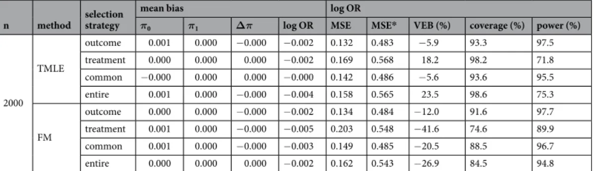
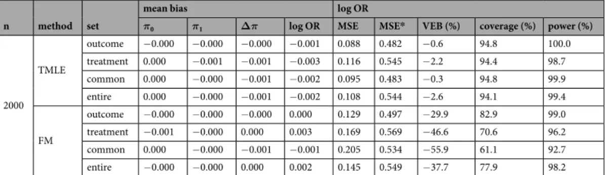
As expected with the common set, the mean absolute bias of θ was close to zero for GC, IPTW and TMLE when the three identifiability assumptions hold with a maximum at −0.028 given moderate sample size (n = 300) under the alternative hypothesis for ATT estimation (Table 1). Note that the three other covariate sets led to a bias close to zero with a maximum of 0.053 for TMLE with the entire set given small sample size (n = 100) under the alternative hypothesis for ATE estimation (Table 2). Furthermore, FM was also associated with a simi-lar bias with a maximum of 0.082 given a small sample size (n = 100), with the treatment set under the alternative hypothesis for the ATE estimation. With an unmeasured confounder, the bias increased in all scenarios with an method selection strategy
mean bias log OR
π0 π1 Δπ log OR MSE MSE* VEB (%) coverage (%) power (%)
100 GC outcome 0.000 −0.001 −0.001 0.012 0.526 0.716 −6.2 94.1 17.7 treatment 0.002 −0.001 −0.003 0.006 0.580 0.786 −5.7 94.1 14.0 common 0.002 −0.001 −0.003 0.006 0.552 0.735 −4.2 94.8 15.1 entire −0.001 −0.001 −0.001 0.013 0.558 0.768 −8.8 93.3 16.9 IPTW outcome 0.000 −0.001 −0.001 0.008 0.578 0.727 10.8 97.3 7.8 treatment −0.000 −0.001 −0.001 0.000 0.716 0.837 −1.2 95.1 9.8 common 0.002 −0.001 −0.003 0.003 0.587 0.743 6.6 96.8 8.8 entire −0.003 −0.001 0.002 0.005 0.741 0.838 −1.5 95.2 9.6 TMLE outcome −0.001 −0.001 0.000 0.002 0.694 0.794 30.0 95.7 5.8 treatment 0.000 −0.001 −0.001 −0.020 0.876 0.955 183.3 98.8 1.0 common −0.000 −0.001 −0.001 −0.001 0.702 0.794 10.4 95.3 7.3 entire −0.003 −0.001 0.001 −0.013 0.886 0.953 412.2 98.8 0.5 FM outcome −0.004 −0.001 0.003 0.022 0.665 0.787 −16.7 90.1 18.9 treatment −0.006 −0.001 0.004 0.017 0.822 0.911 −32.3 81.3 25.2 common −0.001 −0.001 −0.000 0.010 0.653 0.795 −15.3 91.0 17.5 entire −0.008 −0.001 0.006 0.022 0.842 0.921 −33.8 80.3 26.7 300 GC outcome 0.001 −0.001 −0.002 −0.021 0.283 0.555 −1.6 94.5 43.6 treatment 0.002 −0.001 −0.003 −0.024 0.319 0.606 −2.3 94.3 35.2 common 0.002 −0.001 −0.003 −0.023 0.304 0.561 −1.5 94.8 38.5 entire 0.001 −0.001 −0.002 −0.022 0.297 0.600 −2.6 94.0 39.9 IPTW outcome 0.002 −0.001 −0.003 −0.027 0.301 0.556 16.4 97.9 24.0 treatment 0.001 −0.001 −0.002 −0.026 0.372 0.628 6.6 96.2 21.4 common 0.003 −0.001 −0.004 −0.028 0.318 0.563 9.1 96.8 26.1 entire 0.001 −0.001 −0.002 −0.025 0.361 0.622 11.7 97.2 20.0 TMLE outcome 0.000 −0.001 −0.001 −0.023 0.358 0.577 −2.3 93.6 29.0 treatment 0.002 −0.001 −0.003 −0.035 0.454 0.683 51.2 99.1 6.8 common 0.001 −0.001 −0.002 −0.023 0.378 0.582 −3.5 93.0 26.5 entire 0.002 −0.001 −0.003 −0.035 0.432 0.674 81.8 99.3 4.4 FM outcome −0.000 −0.001 −0.001 −0.020 0.351 0.579 −11.7 91.9 37.2 treatment −0.001 −0.001 −0.000 −0.022 0.444 0.656 −30.2 82.7 38.9 common 0.001 −0.001 −0.002 −0.024 0.363 0.587 −14.6 90.4 36.9 entire −0.001 −0.001 0.000 −0.020 0.439 0.662 −29.3 83.2 39.1 500 GC outcome 0.001 −0.001 −0.002 −0.014 0.217 0.509 −1.1 94.7 64.5 treatment 0.001 −0.001 −0.002 −0.014 0.245 0.556 −1.5 94.4 53.6 common 0.001 −0.001 −0.002 −0.015 0.233 0.618 −0.8 94.8 57.6 entire 0.001 −0.001 −0.002 −0.014 0.228 0.552 −2.0 94.2 60.5 IPTW outcome 0.002 −0.001 −0.003 −0.019 0.230 0.509 16.5 97.9 43.3 treatment 0.000 −0.001 −0.001 −0.013 0.285 0.574 6.8 96.6 35.4 common 0.002 −0.001 −0.003 −0.018 0.244 0.514 9.2 96.8 43.7 entire 0.000 −0.001 −0.001 −0.014 0.274 0.571 12.3 97.2 33.9 TMLE outcome 0.001 −0.001 −0.002 −0.015 0.272 0.521 −4.7 93.4 48.5 treatment 0.001 −0.001 −0.002 −0.018 0.347 0.618 35.0 99.1 15.9 common 0.000 −0.001 −0.001 −0.013 0.289 0.527 −4.8 93.1 43.7 entire 0.001 −0.001 −0.002 −0.019 0.328 0.611 51.1 99.3 12.9 FM outcome 0.001 −0.001 −0.002 −0.015 0.265 0.525 −9.9 92.4 53.0 treatment −0.001 −0.001 −0.000 −0.011 0.346 0.597 −31.0 82.7 51.7 common 0.001 −0.001 −0.001 −0.014 0.283 0.530 −15.8 90.1 52.3 entire −0.002 −0.001 0.001 −0.008 0.340 0.596 −29.8 83.2 52.6 2000 GC outcome 0.000 0.000 −0.000 −0.002 0.108 0.479 −1.7 94.7 99.6 treatment 0.001 0.000 −0.000 −0.003 0.122 0.524 −1.2 94.8 98.6 common 0.001 0.000 −0.000 −0.003 0.116 0.480 −0.9 94.7 99.1 entire 0.000 0.000 −0.000 −0.002 0.113 0.523 −1.8 94.5 99.4 IPTW outcome 0.002 0.000 −0.001 −0.006 0.113 0.478 16.3 97.6 98.1 treatment 0.000 0.000 −0.000 −0.002 0.138 0.539 7.9 96.4 93.0 common 0.002 0.000 −0.001 −0.006 0.120 0.480 9.4 97.0 97.7 entire 0.000 0.000 −0.000 −0.002 0.131 0.537 13.9 97.4 93.6 Continued
minimum of 0.456 for GC with the common set given a large sample size for the ATT estimation (see Online Supporting Information (OSI) for complete results). The results were similar under the null hypothesis (see OSI).
Variance.
For all methods, the outcome set led to the lowest MSE, followed closely by the common set. G-computation led to the lowest MSE and FM to the highest. In ATT, IPTW had lower MSE than TMLE. Note that the VEB was particularly high for FM in all ATE scenarios with a minimum of −17.5% (n = 500 with the outcome set). For the ATT, FM also had a higher VEB than other methods, apart from TMLE with the treatment or entire sets in sample sizes of fewer than 2000 subjects. In the presence of an unmeasured confounder, the MSE increased in all scenarios in agreement with the increase in bias. The VEBs did not change notably with an unmeasured confounder.coverage and error rates.
G-computation produced coverage rates close to 95%, except for ATE in a small sample size leading to an anti-conservative 95% CIs with a minimum of 91.7% with the entire set under the null hypothesis. Anti-conservatives 95% CIs were also produced by FM in all scenarios, and by TMLE given a small sample size. Conversely, conservative 95% CIs were obtained when using TMLE for the ATT with the entire or the treatment sets, and when using IPTW for ATT or ATE with the outcome or the common sets.Lending confidence to these results, the type I error was close to 5% for GC in all scenarios and may vary for other methods. The power was more impacted by the choice of the covariate set. The outcome set led to the highest power for GC.
Applications
We illustrated our findings by using two real data sets. First, we compared the efficiency of two treatments, i.e., Natalizumab and Fingolimod, sharing the same indication for active relapsing-remitting multiple sclerosis. Physicians preferentially use Natalizumab in practice for more active disease, indicating possible confounders. Given the absence of a clinical trial with a direct comparison of their efficacy, Barbin et al.53 recently conducted an
observational study. We reused their data. Second, we sought to study barbiturates that can lead to a reduction of the patient functional status. Indeed, barbiturates are suggested in Intensive Care Units (ICU) for the treatment of refractory intracranial pressure increases. However, the use of barbiturates is associated with haemodynamic repercussions that can lead to brain ischaemia and immunodeficiency, which may contribute to the occurrence of infection. These applications were conducted in accordance with the French law relative to clinical noninterven-tional research. According to the French law on Bioethics (July 29, 1994; August 6, 2004; and July 7, 2011, Public Health Code), the patients’ written informed consent was collected. Moreover, data confidentiality was ensured in accordance with the recommendations of the French commission for data protection (Commission Nationale Informatique et Liberté, CNIL decisions DR-2014-558 and DR-2013-047 for the first and the second application, respectively).
To define the four sets of covariates, we asked experts (D.L. for multiple sclerosis and M.L. for ICU) which covariates were causes of the treatment allocation and which were causes of the outcome, as proposed by VanderWeele and Shpitser33. We checked the positivity assumption and the covariate balance (see OSI). We
applied B-spline transformations for continuous variables when the log-linearity assumption did not hold.
natalizumab versus fingolimod to prevent relapse in multiple sclerosis patients.
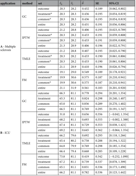
The outcome was at least one relapse within one year of treatment initiation. Six hundred and twenty-nine patients from the French national cohort OFSEP were included (www.ofsep.org). The first part of Table 3 presents a description of their baseline characteristics.All included patients could have received either treatment. Therefore, we sought to estimate the ATE. The first part of Table 4 presents the results according to the different possible methods and covariate sets. The GC, IPTW and TMLE yield similar results regardless of the covariate sets considered. Thus, Fingolimod exhibits lower effi-cacy than Natalizumab with an OR [95% CI] ranging from 1.50 [1.02; 2.21] for IPTW with the entire set to 1.55 [1.06; 2.28] for GC with the common set. When using FM, the OR ranged from 1.73 [1.19; 2.51] with the outcome set to 1.78 [1.23; 2.56] with the common set. Note that, unlike IPTW, FM does not to balance all covariates in the outcome set with standardised differences higher than 10%.
Overall, the confounder-adjusted proportion of patients with at least one relapse within the first year of treatment was lower in the hypothetical world where all patients received Natalizumab (approximately 20% and
n method selection strategy
mean bias log OR
π0 π1 Δπ log OR MSE MSE* VEB (%) coverage (%) power (%)
2000 TMLE outcome 0.001 0.000 −0.000 −0.002 0.132 0.483 −5.9 93.3 97.5 treatment 0.000 0.000 0.000 −0.002 0.169 0.568 18.2 98.2 71.8 common −0.000 0.000 0.000 −0.000 0.142 0.486 −5.6 93.6 95.5 entire 0.001 0.000 −0.000 −0.004 0.158 0.565 23.5 98.6 75.3 FM outcome 0.000 0.000 −0.000 −0.002 0.134 0.484 −12.0 91.6 97.7 treatment 0.001 0.000 −0.000 −0.005 0.203 0.548 −41.6 74.6 89.9 common 0.001 0.000 −0.000 −0.003 0.149 0.485 −20.5 88.5 96.7 entire 0.000 0.000 0.000 −0.002 0.162 0.543 −26.9 84.5 94.8 Table 1. Simulation results comparing the ATT estimation under the alternative hypothesis. *MSE in the presence of an unmeasured confounder. Theoretical values: π1= .0 701,π0= .0 589,θ= .0 492.
n method set
mean bias log OR
π0 π1 Δπ log OR MSE MSE* VEB (%) coverage (%) power (%)
100 GC outcome −0.001 −0.002 −0.001 −0.003 0.404 0.634 −7.3 93.2 24.7 treatment −0.002 −0.001 0.000 0.004 0.477 0.727 −9.5 92.4 19.9 common −0.001 −0.002 −0.001 −0.002 0.434 0.650 −6.6 93.5 22.1 entire −0.002 −0.001 0.001 0.003 0.450 0.714 −11.4 91.8 22.6 IPTW outcome −0.003 −0.001 0.001 0.011 0.464 0.646 12.1 97.4 12.1 treatment −0.006 0.002 0.008 0.046 0.633 0.769 −7.6 93.8 16.7 common −0.002 −0.001 0.001 0.010 0.480 0.657 6.3 96.3 13.5 entire −0.006 0.003 0.009 0.053 0.647 0.773 −7.2 94.7 16.4 TMLE outcome −0.001 −0.002 −0.000 0.003 0.438 0.642 −14.3 89.5 26.9 treatment −0.004 0.002 0.006 0.039 0.572 0.757 −24.9 84.3 27.5 common −0.001 −0.002 −0.001 0.002 0.469 0.657 −10.7 90.9 21.2 entire −0.005 0.003 0.007 0.043 0.544 0.748 −30.7 80.9 34.3 FM outcome −0.005 0.002 0.006 0.039 0.549 0.710 −24.3 87.1 28.5 treatment −0.009 0.005 0.014 0.082 0.677 0.832 −37.7 78.0 35.1 common −0.005 0.001 0.006 0.038 0.563 0.713 −26.3 85.8 29.1 entire −0.007 0.006 0.014 0.082 0.674 0.830 −37.3 78.1 34.8 300 GC outcome −0.000 −0.000 0.000 0.001 0.221 0.532 −1.9 94.5 59.8 treatment −0.000 −0.000 0.000 0.001 0.259 0.608 −2.8 94.3 47.4 common −0.000 −0.000 0.000 0.001 0.237 0.539 −1.2 94.8 53.5 entire −0.000 −0.000 0.000 0.001 0.241 0.600 −3.4 94.0 53.0 IPTW outcome −0.001 −0.000 0.001 0.006 0.239 0.533 20.2 98.0 34.7 treatment −0.002 0.000 0.003 0.014 0.330 0.615 4.6 96.0 29.5 common −0.001 −0.000 0.001 0.006 0.252 0.541 13.3 97.4 36.5 entire −0.002 0.000 0.002 0.013 0.326 0.607 7.9 96.6 28.5 TMLE outcome −0.000 −0.001 −0.000 0.000 0.233 0.532 −3.0 93.9 54.2 treatment −0.001 0.000 0.002 0.009 0.310 0.612 −10.4 90.6 40.2 common −0.001 −0.001 0.000 0.001 0.249 0.540 −1.5 94.6 48.1 entire −0.001 0.000 0.001 0.008 0.290 0.603 −13.2 89.6 46.1 FM outcome −0.002 0.000 0.002 0.010 0.294 0.552 −20.2 88.7 51.6 treatment −0.003 0.003 0.006 0.032 0.389 0.652 −39.3 77.0 53.3 common −0.001 −0.000 0.001 0.008 0.315 0.588 −25.5 86.2 51.3 entire −0.003 0.003 0.006 0.032 0.377 0.644 −37.4 77.8 52.2 500 GC outcome −0.000 0.000 0.001 0.003 0.168 0.501 −0.4 94.8 81.1 treatment −0.000 0.000 0.001 0.002 0.198 0.573 −1.0 94.8 69.0 common −0.000 0.000 0.000 0.002 0.183 0.505 −0.7 94.9 75.0 entire −0.000 0.000 0.001 0.004 0.183 0.569 −1.0 94.8 75.3 IPTW outcome −0.001 0.000 0.001 0.005 0.180 0.501 22.2 98.3 58.5 treatment −0.001 0.001 0.001 0.007 0.248 0.573 8.1 96.5 42.3 common −0.001 0.000 0.001 0.005 0.193 0.505 13.8 97.3 58.6 entire −0.001 0.000 0.001 0.006 0.239 0.569 13.1 97.2 41.3 TMLE outcome −0.000 0.000 0.000 0.002 0.177 0.501 −0.8 94.7 76.8 treatment −0.000 0.000 0.000 0.003 0.234 0.571 −5.9 92.7 56.1 common −0.000 0.000 0.000 0.002 0.190 0.505 −0.5 94.7 69.7 entire −0.000 0.000 0.000 0.003 0.218 0.566 −7.5 91.8 63.1 FM outcome −0.001 0.000 0.001 0.005 0.219 0.518 −17.5 89.8 70.1 treatment −0.002 0.002 0.003 0.018 0.302 0.598 −39.8 76.2 65.5 common −0.001 −0.000 0.001 0.005 0.266 0.555 −31.8 82.3 66.4 entire −0.002 0.002 0.004 0.019 0.289 0.592 −37.1 78.3 66.2 2000 GC outcome −0.000 −0.000 −0.000 −0.001 0.085 0.482 −0.6 94.6 100.0 treatment 0.000 −0.001 −0.001 −0.003 0.099 0.550 −0.6 94.7 99.8 common 0.000 −0.001 −0.001 −0.003 0.092 0.483 −0.8 94.7 99.9 entire −0.000 −0.000 −0.000 −0.001 0.091 0.550 −0.6 94.7 99.9 IPTW outcome −0.000 −0.000 0.000 0.002 0.090 0.482 21.2 98.2 99.8 treatment 0.000 −0.001 −0.001 −0.002 0.122 0.547 9.3 96.7 95.1 common −0.000 −0.000 0.000 0.001 0.096 0.483 13.5 97.3 99.7 entire 0.000 −0.000 −0.001 −0.002 0.117 0.546 14.3 97.5 95.6 Continued
varying slightly depending on method and set of covariates) than one in which all patients received Fingolimod (approximately 28%). This difference of approximately 8% is clinically meaningful and suggests the superiority of Natalizumab over Fingolimod to prevent relapses at one year. This result was concordant with the recent clinical literature53,54.
impact of barbiturates in the icU on the functional status at three months.
We define an unfa-vourable functional outcome by a 3-month Glasgow Outcome Scale (GOS) lower than or equal to 3. We used the data from the French observational cohort AtlanREA (www.atlanrea.org) to estimate the ATT of barbiturates because physicians recommended these drugs to a minority of severe patients. The second part of Table 3 presents the baseline characteristics of the 252 included patients.The second part of Table 4 presents the results according to the different possible methods and covariate sets. G-computation and TMLE lead to the conclusion of a significant negative effect of barbiturates regardless of the covariate set considered with an OR [95% CI] ranging from 0.43 [0.25; 0.76] for GC with the common set to 0.51 [0.29; 0.90] for TMLE with the entire set. By contrast, the results were discordant when using different covari-ate sets for IPTW and FM. We report, for instance, OR estimcovari-ates obtained by FM ranging from 1.520 with the outcome set to 2.300 with the common set. In line with the simulation study, the estimated standard errors were higher for these methods (0.294 and 0.293 for GC and TMLE when the outcome set was considered, respectively) leading to lower power. Note also that standardised differences were higher than 10% for the IPTW with the entire set (see OSI) and for FM with the outcome, the treatment and the entire sets.
Depending on the methods and sets of covariates included, we estimated that from 18% to 20% of patients treated with barbiturates had an unfavourable GOS at three months. If these patients had not received barbitu-rates, the methods estimate that from 30% to 35% would have had an unfavourable GOS at three months. For the patients, this difference is meaningful but full clinical relevance depends also on the effect of barbiturates on other clinically relevant outcomes, such as death or ventilator-associated pneumonia. However, the results obtained by GC or TMLE differ with those obtained by Majdan et al.55, who did not find any significant effect of barbiturates
on the GOS at six months. Two main methodological reasons can explain this difference: the GOS was at six months rather than three months post-initiation, and the authors used multivariate logistic regression leading to a different estimand.
Discussion
The aim of this study was to better understand the different sets of covariates to consider when estimating the marginal causal effect.
The results of our simulation study, limited to the studied scenarios, highlight that the use of the outcome set was associated with the lower bias and variance, principally when associated with GC, for both ATE and ATT. As expected, an unmeasured confounder led to increased bias, regardless of method employed. Although we do not report an impact on the variance, the effect’s over- or under-estimation leads to the corresponding over- or under-estimation of power and compromises the validity of the causal inference.
The performance of FM is lower than that of the other studied methods, especially for the variance. Our results were in line with King and Nielsen56, who argued for halting the use of PS matching for many reasons such as
covariate imbalance, inefficiency, model dependence and bias. Nonetheless, Colson et al.17 found slightly higher
MSE for GC than FM. Their more simplistic scenario, with only two simulated confounders leading to little covar-iate imbalance, could explain the difference with our results. Moreover, is unclear whether they accounted for the matched nature of the data, as recommended by Austin and Stuart16 or Gayat et al.50.
While DRE offers protection against model misspecification23,34,36, our simulation study resulted in the finding
that GC was more robust to the choice of the covariate set than the other methods, TMLE included. This result was particularly important when the treatment set was taken into account, which fits with the results of Kang and Schafer35: when both the PS and the Q-model were misspecified, DRE had lower performance than GC.
Furthermore, GC was associated with lower variance than DRE in several simulation studies13,17,35, which accords
with our results.
The first application to multiple sclerosis (ATE) illustrated similar results between the studied methods. In contrast, the second application (ATT) to severe trauma or brain-damaged patients showed different results between the methods. In agreement with simulations, the estimations obtained with GC or TMLE were similar
n method set
mean bias log OR
π0 π1 Δπ log OR MSE MSE* VEB (%) coverage (%) power (%)
2000 TMLE outcome −0.000 −0.000 −0.000 −0.001 0.088 0.482 −0.6 94.8 100.0 treatment 0.000 −0.001 −0.001 −0.003 0.116 0.545 −2.2 94.4 98.7 common 0.000 −0.000 −0.001 −0.002 0.095 0.483 −0.3 94.8 99.9 entire 0.000 −0.000 −0.001 −0.002 0.108 0.544 −2.6 94.1 99.4 FM outcome −0.000 −0.000 −0.000 0.000 0.129 0.497 −29.9 82.9 99.0 treatment −0.001 −0.000 0.000 0.003 0.169 0.569 −46.6 70.6 96.2 common 0.000 −0.000 −0.001 −0.001 0.205 0.534 −55.9 61.1 92.7 entire −0.000 −0.000 0.000 0.002 0.145 0.549 −37.7 77.9 98.2 Table 2. Simulation results comparing the ATE estimation under the alternative hypothesis. *MSE in the presence of an unmeasured confounder. Theoretical values: π1= .0 557,π0= .0 441,θ= .0 466.
in terms of logOR estimation and variance regardless of the covariate set considered. Estimations obtained with IPTW or FM were highly variable, depending on the covariate set employed: some indicated a negative impact of barbiturates and others did not. These results also tended to demonstrate that GC or TMLE had the highest statistical power. Variances obtained by parametric simulations or by bootstrap resampling were similar (results not displayed).
One can, therefore, question the relative predominance of the PS-based approach compared to GC, although there are several potential explanations. First, there appears to be a pre-conceived notion according to which multivariable non-linear regression cannot be used to estimate marginal absolute and relative effects57. Indeed,
under logistic regression, the mean sample probability of an event is different from the event probability of a subject with the mean sample characteristics. Second, while there is an explicit variance formula for the IPTW58,
the equivalent is missing for the GC. The variance must be obtained by bootstrapping, simulation or the delta method. Third, several didactic tutorials on PS-based methods can be found, for instance59–61.
We still believe that PS-based methods may have value when multivariate modelling is complex, for instance, for multi-state models62. In future research, it would be interesting to examine whether the use of potentially
bet-ter settings would provide equivalent results, such as the Williamson estimator for IPTW58, the Abadie-Imbens
estimator for PS matching63, or bounded the estimation of TMLE, which can also be updated several times36. We
also emphasise that we did not investigate these methods when the positivity assumption does not hold. Several authors have studied this problem13,25,35,36,64. G-computation was less biased than IPTW or DRE except in Porter
et al.36, where the violation of the positivity assumption was also associated with model misspecifications. The
robustness of GC to non-positivity could be due to a correct extrapolation into the missing sub-population, which is not feasible with PS1. Other perspectives of this work are to extend the problem to i) time-to-event, continuous
or multinomial outcomes and ii) multinomial treatment. However, implementing GC using continuous treatment raises many important considerations concerning the research question and resulting inference64.
A - Multiple sclerosis Overall (n = 629)
First line treatment Relapse at 1 year
Ntz (n = 326) Fng (n = 303) p No (n = 478) Yes (n = 151) p Patient age, years (mean, sd) 37.0 9.6 36.8 9.9 37.2 9.2 0.6505 37.1 9.7 36.6 9.2 0.5849 Female patient (n, %) 479.0 76.2 254.0 77.9 225.0 74.3 0.2822 367.0 76.8 112.0 74.2 0.5124 Disease duration, years (mean, sd) 8.5 6.4 8.0 6.1 9.0 6.8 0.0505 8.6 6.6 8.2 6.0 0.4809 At least one relapse (n, %) 526.0 83.6 293.0 89.9 233.0 76.9 <0.0001 391.0 81.8 135.0 89.4 0.0277 Gd-enhancing lesion on MRI (n, %) 311.0 49.4 185.0 56.7 126.0 41.6 0.0001 240.0 50.2 71.0 47.0 0.4944 EDSS score >3 (n, %) 288.0 45.8 166.0 50.9 122.0 40.3 0.0074 212.0 44.4 76.0 50.3 0.1986 Previous immunomodulatory treatment (n, %) 556.0 88.4 293.0 89.9 263.0 86.8 0.2284 424.0 88.7 132.0 87.4 0.6672 B – ICU Overall (n = 252) Barbiturates treatment Favourable GOS at 3 months
No (n = 178) Yes (n = 74) p No (n = 180) Yes (n = 72) p Patient age, years (mean, sd) 47.4 17.4 48.7 17.9 44.1 15.7 0.0565 50.8 16.4 38.7 16.9 <0.0001 Female patient (n, %) 89.0 35.3 58.0 32.6 31.0 41.9 0.1592 68.0 37.8 21.0 29.2 0.1963
Diabetes (n, %) 17.0 6.7 15.0 8.4 2.0 2.7 0.0989 15.0 8.3 2.0 2.8 0.1122
Nosological entity: Severe trauma (n, %) 124.0 49.2 95.0 53.4 29.0 39.2 0.0403 77.0 42.8 47.0 65.3 0.0012 SAP ≤90 mmHg before admission (n, %) 56.0 22.2 36.0 20.2 20.0 27.0 0.2368 46.0 25.6 10.0 13.9 0.0442 Evacuation of subdural or extradural hematoma (n, %) 41.0 16.3 33.0 18.5 8.0 10.8 0.1301 27.0 15.0 14.0 19.4 0.3878 External ventricular drain (n, %) 64.0 25.4 39.0 21.9 25.0 33.8 0.0486 48.0 26.7 16.0 22.2 0.4640 Evacuation of cerebral hematoma or lobectomy (n, %) 42.0 16.7 28.0 15.7 14.0 18.9 0.5362 34.0 18.9 8.0 11.1 0.1345 Decompressive craniectomy (n, %) 27.0 10.7 15.0 8.4 12.0 16.2 0.0686 21.0 11.7 6.0 8.3 0.4396 Blood transfusion before admission (n, %) 34.0 13.5 25.0 14.0 9.0 12.2 0.6903 26.0 14.4 8.0 11.1 0.4841 Pneumonia before increased ICP (n, %) 29.0 11.5 16.0 9.0 13.0 17.6 0.0519 19.0 10.6 10.0 13.9 0.4538 Osmotherapy (n, %) 112.0 44.4 75.0 42.1 37.0 50.0 0.2525 89.0 49.4 23.0 31.9 0.0115 GCS score ≥8 62.0 24.6 39.0 21.9 23.0 31.1 0.1237 37.0 20.6 25.0 34.7 0.0183 Hemoglobin, g/dL (mean, sd) 11.8 2.3 11.7 2.2 12.1 2.5 0.1824 11.8 2.4 11.9 1.9 0.7373 Platelets, counts/mm3 (mean, sd) 206.7 78.0 207.4 79.7 205.1 74.2 0.8312 209.0 83.8 200.9 61.1 0.4589
Serum creatinine, mmol/L (mean, sd) 71.1 29.3 71.1 27.6 71.1 33.3 0.9853 72.4 32.6 67.9 18.7 0.2732 Arterial pH (mean, sd) 7.3 0.1 7.3 0.1 7.3 0.1 0.0978 7.3 0.1 7.3 0.1 0.6317 Serum proteins, g/L (mean, sd) 58.2 10.4 57.7 10.6 59.6 9.7 0.1662 58.0 10.7 58.8 9.7 0.5963 Serum urea, mmol/L (mean, sd) 5.0 2.5 5.2 2.7 4.7 1.8 0.1827 5.2 2.3 4.5 2.9 0.0505 PaO2/FiO2 ratio (mean, sd) 302.7 174.0 292.7 154.7 326.6 212.9 0.1595 282.1 172.4 354.2 168.4 0.0028
SAPS II score (mean, sd) 47.6 11.4 47.6 10.7 47.6 12.9 0.9847 49.9 10.8 41.8 10.7 <0.0001 Table 3. Baseline characteristics of patients of the two studied cohorts. Ntz: Natalizumab, Fng: Fingolimod,
Gd: Gadolinium, MRI: Magnetic Resonance Imaging, EDSS: Expanded Disability Status Scale, SAP: Systolic Arterial Pressure, ICP: Intra-Cranial Pressure, GCS: Glasgow Coma Scale, PaO2/FiO2: arterial partial Pressure
To facilitate its use in practice, we have implemented the estimation of both ATE and ATT, and their 95% CI, from a logistic model in the existing R package entitled RISCA (available at cran.r-project.org/web/packages/ RISCA). We provide an example of R code in the appendix. Note that the package did not consider the inflation of the type I error rate due to the modelling steps of the Q-model. Users also have to consider novel strategies for post-model selection inference.
In the applications, we classified covariates into sets based on experts knowledge33. However, several statistical
methods can be useful when no clinical knowledge is available. Heinze et al.65 proposed a review of the most used,
while Witte and Didelez66 reviewed strategies specific to causal inference. Alternatively, data-adaptive methods
have recently been developed, such as the outcome-adaptive LASSO67 to select covariates associated with both
the outcome and the treatment allocation. Nevertheless, according to our results, it may be preferable to focus on constructing the best outcome model based on the outcome set. For instance, the consideration of a super learner68,69, merging models and modelling machine learning algorithms may represent an exciting perspective70.
Finally, we emphasise that the conclusions from our simulation study cannot be generalised to all situations. They are consistent with the current literature on causal inference, but theoretical arguments are missing for gen-eralisation. Notably, our results must be considered in situations where both the PS and the Q-model are correctly specified and where positivity holds.
To conclude, we demonstrate in a simulation study that adjusting for all the covariates causing the outcome improves the estimation of the marginal causal effect (ATE or ATT) of a binary treatment in a binary outcome. Considering only the covariates that are a common cause of both the outcome and the treatment is possible when the number of potential confounders is large. The strategy consisting of considering all available covariates,
i.e., no selection, did not decrease the bias but significantly decreased the power. Amongst the different studied
methods, GC had the lowest bias and variance regardless of covariate set considered. Consequently, we recom-mend that the use of the GC with the outcome set, because of its highest power in all the simulated scenarios. For
application method set πˆ0 πˆ1 θˆ SE 95% CI
A - Multiple sclerosis GC outcome 20.3 28.2 0.432 0.189 [0.062, 0.802] treatment* 20.3 28.3 0.436 0.195 [0.054, 0.819] common* 20.3 28.3 0.436 0.195 [0.054, 0.819] entire 20.3 28.2 0.431 0.191 [0.056, 0.806] IPTW outcome 21.2 28.8 0.406 0.195 [0.023, 0.789] treatment* 20.3 28.2 0.433 0.191 [0.059, 0.808] common* 20.3 28.2 0.433 0.191 [0.059, 0.808] entire 21.3 28.9 0.406 0.196 [0.022, 0.791] TMLE outcome 21.2 28.8 0.407 0.195 [0.025, 0.790] treatment* 20.3 28.2 0.433 0.190 [0.061, 0.806] common* 20.3 28.2 0.433 0.190 [0.061, 0.806] entire 21.1 28.9 0.410 0.196 [0.026, 0.794] FM outcome 19.1 29.0 0.549 0.189 [0.178, 0.921] treatment* 19.9 30.6 0.575 0.187 [0.210, 0.941] common* 19.9 30.6 0.575 0.187 [0.210, 0.941] entire 21.1 31.9 0.561 0.183 [0.201, 0.920] B - ICU GC outcome 66.3 81.1 0.778 0.294 [0.201, 1.354] treatment 65.3 81.1 0.824 0.298 [0.240, 1.407] common 65.0 81.1 0.836 0.289 [0.270, 1.402] entire 66.5 81.1 0.769 0.295 [0.191, 1.347] IPTW outcome 31.0 81.1 0.656 0.356 [−0.042, 1.354] treatment 68.2 81.1 0.693 0.355 [−0.002, 1.388] common 67.4 81.1 0.729 0.353 [0.038, 1.421] entire 69.2 81.1 0.645 0.362 [−0.064, 1.354] TMLE outcome 66.2 79.6 0.692 0.293 [0.118, 1.266] treatment 65.4 80.2 0.758 0.288 [0.194, 1.322] common 64.8 79.9 0.769 0.298 [0.185, 1.354] entire 66.4 79.4 0.668 0.285 [0.109, 1.228] FM outcome 73.8 81.1 0.419 0.342 [−0.252, 1.090] treatment 67.2 81.1 0.739 0.337 [0.078, 1.399] common 65.1 81.1 0.831 0.336 [0.173, 1.490] entire 66.2 81.1 0.782 0.336 [0.123, 1.442]
Table 4. Results of the two applications. *Treatment and common sets contain same covariates. π0: Percentage
of event in the Natalizumab (or control) group, π1: Percentage of event in the Fingolimod (or Barbiturates)
instance, at least 500 individuals were necessary to achieve a power higher than 80% in ATE, with a theoretical OR at 2, and a percentage of treated subjects at 50%. In ATT, we needed larger sample size to reach a power of 80% because the estimation considers only the treated patients. With 2000 individuals, all the studied methods with the outcome set led to a bias close to zero and a statistical power superior to 95%.
Received: 9 July 2019; Accepted: 26 April 2020; Published: xx xx xxxx
References
1. Hernan, M. A. & Robins, J. M. Causal Inference: What if? (Chapman & Hall/CRC, 2020).
2. Zwarenstein, M. & Treweek, S. What kind of randomized trials do we need? Journal of Clinical Epidemiology 62, 461–463, https:// doi.org/10.1016/j.jclinepi.2009.01.011 (2009).
3. Gayat, E. et al. Propensity scores in intensive care and anaesthesiology literature: a systematic review. Intensive Care Medicine 36, 1993–2003, https://doi.org/10.1007/s00134-010-1991-5 (2010).
4. Rosenbaum, P. R. & Rubin, D. B. The central role of the propensity score in observational studies for causal effects. Biometrika 70, 41–55, https://doi.org/10.2307/2335942 (1983).
5. Robins, J. M., Hernán, M. A. & Brumback, B. Marginal structural models and causal inference in epidemiology. Epidemiology 11, 550–560, https://doi.org/10.1097/00001648-200009000-00011 (2000).
6. Lunceford, J. K. & Davidian, M. Stratification and weighting via the propensity score in estimation of causal treatment effects: a comparative study. Statistics in medicine 23, 2937–2960, https://doi.org/10.1002/sim.1903 (2004).
7. Austin, P. C., Grootendorst, P., Normand, S.-L. T. & Anderson, G. M. Conditioning on the propensity score can result in biased estimation of common measures of treatment effect: a Monte Carlo study. Statistics in Medicine 26, 754–768, https://doi.org/10.1002/ sim.2618 (2007).
8. Abdia, Y., Kulasekera, K. B., Datta, S., Boakye, M. & Kong, M. Propensity scores based methods for estimating average treatment effect and average treatment effect among treated: A comparative study. Biometrical Journal 59, 967–985, https://doi.org/10.1002/ bimj.201600094 (2017).
9. Grose, E. et al. Use of propensity score methodology in contemporary high-impact surgical literature. Journal of the American
College of Surgeons 230, 101–112.e2, https://doi.org/10.1016/j.jamcollsurg.2019.10.003 (2020).
10. Ali, M. S. et al. Reporting of covariate selection and balance assessment in propensity score analysis is suboptimal: a systematic review. Journal of Clinical Epidemiology 68, 112–121, https://doi.org/10.1016/j.jclinepi.2014.08.011 (2015).
11. Le Borgne, F., Giraudeau, B., Querard, A. H., Giral, M. & Foucher, Y. Comparisons of the performance of different statistical tests for time-to-event analysis with confounding factors: practical illustrations in kidney transplantation. Statistics in Medicine 35, 1103–1116, https://doi.org/10.1002/sim.6777 (2016).
12. Hajage, D., Tubach, F., Steg, P. G., Bhatt, D. L. & De Rycke, Y. On the use of propensity scores in case of rare exposure. BMC Medical
Research Methodology 16, https://doi.org/10.1186/s12874-016-0135-1 (2016).
13. Lendle, S. D., Fireman, B. & van der Laan, M. J. Targeted maximum likelihood estimation in safety analysis. Journal of Clinical
Epidemiology 66, S91–S98, https://doi.org/10.1016/j.jclinepi.2013.02.017 (2013).
14. Austin, P. C. The performance of different propensity-score methods for estimating differences in proportions (risk differences or absolute risk reductions) in observational studies. Statistics in Medicine 29, 2137–2148, https://doi.org/10.1002/sim.3854 (2010). 15. Austin, P. C. & Stuart, E. A. Estimating the effect of treatment on binary outcomes using full matching on the propensity score.
Statistical Methods in Medical Research 26, 2505–2525, https://doi.org/10.1177/0962280215601134 (2017).
16. Austin, P. C. & Stuart, E. A. The performance of inverse probability of treatment weighting and full matching on the propensity score in the presence of model misspecification when estimating the effect of treatment on survival outcomes. Statistical Methods in
Medical Research 26, 1654–1670, https://doi.org/10.1177/0962280215584401 (2017).
17. Colson, K. E. et al. Optimizing matching and analysis combinations for estimating causal effects. Scientific Reports 6, https://doi. org/10.1038/srep23222 (2016).
18. Robins, J. M. A new approach to causal inference in mortality studies with a sustained exposure period-application to control of the healthy worker survivor effect. Mathematical Modelling 7, 1393–1512, https://doi.org/10.1016/0270-0255(86)90088-6 (1986). 19. Vansteelandt, S. & Keiding, N. Invited commentary: G-computation-lost in translation? American Journal of Epidemiology 173,
739–742, https://doi.org/10.1093/aje/kwq474 (2011).
20. Snowden, J. M., Rose, S. & Mortimer, K. M. Implementation of g-computation on a simulated data set: Demonstration of a causal inference technique. American Journal of Epidemiology 173, 731–738, https://doi.org/10.1093/aje/kwq472 (2011).
21. Wang, A., Nianogo, R. A. & Arah, O. A. G-computation of average treatment effects on the treated and the untreated. BMC Medical
Research Methodology 17, https://doi.org/10.1186/s12874-016-0282-4 (2017).
22. Imbens, G. W. Nonparametric estimation of average treatment effects under exogeneity: A review. The Review of Economics and
Statistics 86, 4–29, https://doi.org/10.1162/003465304323023651 (2004).
23. Bang, H. & Robins, J. M. Doubly robust estimation in missing data and causal inference models. Biometrics 61, 962–973, https://doi. org/10.1111/j.1541-0420.2005.00377.x (2005).
24. van der Laan, M. J. & Rubin, D. B. Targeted maximum likelihood learning. The International Journal of Biostatistics 2, https://doi. org/10.2202/1557-4679.1043 (2006).
25. Neugebauer, R. & van der Laan, M. J. Why prefer double robust estimators in causal inference? Journal of Statistical Planning and
Inference 129, 405–426, https://doi.org/10.1016/j.jspi.2004.06.060 (2005).
26. Brookhart, M. A. et al. Variable Selection for Propensity Score Models. American Journal of Epidemiology 163, 1149–1156, https:// doi.org/10.1093/aje/kwj149 (2006).
27. Lefebvre, G., Delaney, J. A. C. & Platt, R. W. Impact of mis-specification of the treatment model on estimates from a marginal structural model. Statistics in Medicine 27, 3629–3642, https://doi.org/10.1002/sim.3200 (2008).
28. Schisterman, E. F., Cole, S. R. & Platt, R. W. Overadjustment bias and unnecessary adjustment in epidemiologic studies.
Epidemiology 20, 488–495, https://doi.org/10.1097/EDE.0b013e3181a819a1 (2009).
29. Rotnitzky, A., Li, L. & Li, X. A note on overadjustment in inverse probability weighted estimation. Biometrika 97, 997–1001, https:// doi.org/10.1093/biomet/asq049 (2010).
30. Schnitzer, M. E., Lok, J. J. & Gruber, S. Variable selection for confounder control, flexible modeling and collaborative targeted minimum loss-based estimation in causal inference. The International Journal of Biostatistics 12, 97–115, https://doi.org/10.1515/ ijb-2015-0017 (2016).
31. Myers, J. A. et al. Effects of adjusting for instrumental variables on bias and precision of effect estimates. American Journal of
Epidemiology 174, 1213–1222, https://doi.org/10.1093/aje/kwr364 (2011).
32. De Luna, X., Waernbaum, I. & Richardson, T. S. Covariate selection for the nonparametric estimation of an average treatment effect.
Biometrika 98, 861–875, https://doi.org/10.1093/biomet/asr041 (2011).
33. VanderWeele, T. J. & Shpitser, I. A new criterion for confounder selection. Biometrics 67, 1406–1413, https://doi.org/10.1111/j.1541-0420.2011.01619.x (2011).
34. Schuler, M. S. & Rose, S. Targeted maximum likelihood estimation for causal inference in observational studies. American Journal
of Epidemiology 185, 65–73, https://doi.org/10.1093/aje/kww165 (2017).
35. Kang, J. D. Y. & Schafer, J. L. Demystifying double robustness: A comparison of alternative strategies for estimating a population mean from incomplete data. Statistical Science 22, 523–539, https://doi.org/10.1214/07-STS227 (2007).
36. Porter, K. E., Gruber, S., van der Laan, M. J. & Sekhon, J. S. The relative performance of targeted maximum likelihood estimators. The
International Journal of Biostatistics 7, https://doi.org/10.2202/1557-4679.1308 (2011).
37. Moher, D. et al. Consort 2010 explanation and elaboration: updated guidelines for reporting parallel group randomised trials. BMJ 340, c869, https://doi.org/10.1136/bmj.c869 (2010).
38. Greenland, S., Robins, J. M. & Pearl, J. Confounding and collapsibility in causal inference. Statistical Science 14, 29–46, https://doi. org/10.1214/ss/1009211805 (1999).
39. Aalen, O. O., Cook, R. J. & Røysland, K. Does cox analysis of a randomized survival study yield a causal treatment effect? Lifetime
Data Analysis 21, 579–593, https://doi.org/10.1007/s10985-015-9335-y (2015).
40. Pearl, J., Glymour, M. & Jewell, N. P. Causal Inference in Statistics: A Primer (John Wiley & Sons, 2016).
41. Xu, S. et al. Use of Stabilized Inverse Propensity Scores as Weights to Directly Estimate Relative Risk and Its Confidence Intervals.
Value in Health 13, 273–277, https://doi.org/10.1111/j.1524-4733.2009.00671.x (2010).
42. Morgan, S. L. & Todd, J. J. A diagnostic routine for the detection of consequential heterogeneity of causal effects. Sociological
Methodology 38, 231–282, https://doi.org/10.1111/j.1467-9531.2008.00204.x (2008).
43. Zeileis, A. Object-oriented computation of sandwich estimators. Journal of Statistical Software 16, 1–16, https://doi.org/10.18637/ jss.v016.i09 (2006).
44. Austin, P. C. The use of propensity score methods with survival or time-to-event outcomes: reporting measures of effect similar to those used in randomized experiments: Propensity scores and survival analysis. Statistics in Medicine 33, 1242–1258, https://doi. org/10.1002/sim.5984 (2014).
45. Ho, D., Imai, K., King, G. & Stuart, E. MatchIt: Nonparametric Preprocessing for Parametric Causal Inference. Journal of Statistical
Software 42, 1–28, https://doi.org/10.18637/jss.v042.i08 (2011).
46. Aalen, O. O., Farewell, V. T., De Angelis, D., Day, N. E. & Gill, O. N. A markov model for hiv disease progression including the effect of hiv diagnosis and treatment: application to aids prediction in england and wales. Statistics in Medicine 16, 2191–2210, https://doi. org/10.1002/(sici)1097-0258(19971015)16:19<2191::aid-sim645>3.0.co;2-5 (1997).
47. van der Laan, M. J. & Rose, S. Targeted learning: causal inference for observational and experimental data. Springer series in statistics (Springer, 2011).
48. Hampel, F. R. The influence curve and its role in robust estimation. Journal of the American Statistical Association 69, 383–393,
https://doi.org/10.2307/2285666 (1974).
49. Luque-Fernandez, M. A., Schomaker, M., Rachet, B. & Schnitzer, M. E. Targeted maximum likelihood estimation for a binary treatment: A tutorial. Statistics in Medicine 37, 2530–2546, https://doi.org/10.1002/sim.7628 (2018).
50. Gayat, E., Resche-Rigon, M., Mary, J.-Y. & Porcher, R. Propensity score applied to survival data analysis through proportional hazards models: a Monte Carlo study. Pharmaceutical Statistics 11, 222–229, https://doi.org/10.1002/pst.537 (2012).
51. Morris, T. P., White, I. R. & Crowther, M. J. Using simulation studies to evaluate statistical methods. Statistics in Medicine 38, 2074–2102, https://doi.org/10.1002/sim.8086 (2019).
52. R Core Team. R: A Language and Environment for Statistical Computing. (R Foundation for Statistical Computing, Vienna, Austria, 2014).
53. Barbin, L. et al. Comparative efficacy of fingolimod vs natalizumab. Neurology 86, 771–778, https://doi.org/10.1212/
WNL.0000000000002395 (2016).
54. Kalincik, T. et al. Switch to natalizumab versus fingolimod in active relapsing-remitting multiple sclerosis. Annals of Neurology 77, 425–435, https://doi.org/10.1002/ana.24339 (2015).
55. Majdan, M. et al. Barbiturates Use and Its Effects in Patients with Severe Traumatic Brain Injury in Five European Countries. Journal
of Neurotrauma 30, 23–29, https://doi.org/10.1089/neu.2012.2554 (2012).
56. King, G. & Nielsen, R. Why propensity scores should not be used for matching. Political Analysis 27, 435–454, https://doi. org/10.1017/pan.2019.11 (2019).
57. Nieto, F. J. & Coresh, J. Adjusting survival curves for confounders: a review and a new method. American Journal of Epidemiology 143, 1059–1068, https://doi.org/10.1093/oxfordjournals.aje.a008670 (1996).
58. Williamson, E. J., Forbes, A. & White, I. R. Variance reduction in randomised trials by inverse probability weighting using the propensity score. Statistics in Medicine 33, 721–737, https://doi.org/10.1002/sim.5991 (2014).
59. Williamson, E. J., Morley, R., Lucas, A. & Carpenter, J. Propensity scores: From naïve enthusiasm to intuitive understanding.
Statistical Methods in Medical Research 21, 273–293, https://doi.org/10.1177/0962280210394483 (2012).
60. Austin, P. C. An Introduction to Propensity Score Methods for Reducing the Effects of Confounding in Observational Studies.
Multivariate Behavioral Research 46, 399–424, https://doi.org/10.1080/00273171.2011.568786 (2011).
61. Haukoos, J. S. & Lewis, R. J. The propensity score. JAMA 314, 1637–1638, https://doi.org/10.1001/jama.2015.13480 (2015). 62. Gillaizeau, F. et al. Inverse probability weighting to control confounding in an illness-death model for interval-censored data.
Statistics in Medicine 37, 1245–1258, https://doi.org/10.1002/sim.7550 (2018).
63. Abadie, A. & Imbens, G. W. Large sample properties of matching estimators for average treatment effects. Econometrica 74, 235–267,
https://doi.org/10.1111/j.1468-0262.2006.00655.x (2006).
64. Moore, K. L., Neugebauer, R., van der Laan, M. J. & Tager, I. B. Causal inference in epidemiological studies with strong confounding.
Statistics in Medicine 31, 1380–1404, https://doi.org/10.1002/sim.4469 (2012).
65. Heinze, G., Wallisch, C. & Dunkler, D. Variable selection - a review and recommendations for the practicing statistician. Biometrical
Journal 60, 431–449, https://doi.org/10.1002/bimj.201700067 (2018).
66. Witte, J. & Didelez, V. Covariate selection strategies for causal inference: Classification and comparison. Biometrical Journal 61, 1270–1289, https://doi.org/10.1002/bimj.201700294 (2019).
67. Shortreed, S. M. & Ertefaie, A. Outcome-adaptive lasso: variable selection for causal inference. Biometrics 73, 1111–1122, https://doi. org/10.1111/biom.12679 (2017).
68. van der Laan, M. J., Polley, E. C. & Hubbard, A. E. Super learner. Statistical Applications in Genetics and Molecular Biology 6, Article 25, https://doi.org/10.2202/1544-6115.1309 (2007).
69. Naimi, A. I. & Balzer, L. B. Stacked generalization: An introduction to super learning. European journal of epidemiology 33, 459–464,
https://doi.org/10.1007/s10654-018-0390-z (2018).
70. Pirracchio, R. & Carone, M. The balance super learner: A robust adaptation of the super learner to improve estimation of the average treatment effect in the treated based on propensity score matching. Statistical Methods in Medical Research 27, 2504–2518, https:// doi.org/10.1177/0962280216682055 (2018).
Acknowledgements
The authors would like to thank the members of AtlanREA and OFSEP Groups for their involvement in the study, the physicians who helped recruit patients and all patients who participated in this study. We also thank the clinical research associates who participated in the data collection. The analysis and interpretation of these data are the responsibility of the authors. This work was partially supported by a public grant overseen by the