Universit´e de Montr´eal
Improved Training of Energy-Based Models
par Rithesh Kumar
D´epartement d’informatique et de recherche op´erationnelle Facult´e des arts et des sciences
M´emoire pr´esent´e `a la Facult´e des arts et des sciences en vue de l’obtention du grade de Maˆıtre `es sciences (M.Sc.)
en informatique
June, 2019
Universit´e de Montr´eal Facult´e des arts et des sciences
Ce m´emoire intitul´e:
Improved Training of Energy-Based Models
pr´esent´e par: Rithesh Kumar
a ´et´e ´evalu´e par un jury compos´e des personnes suivantes: Stefan Monnier, pr´esident-rapporteur
Yoshua Bengio, directeur de recherche Neil Stewart, membre du jury
Résumé
L’estimation du maximum de vraisemblance des mod`eles bas´es sur l’´energie est un probl`eme difficile `a r´esoudre en raison de l’insolubilit´e du gradient du logarith-mique de la vraisemblance. Dans ce travail, nous proposons d’apprendre `a la fois la fonction d’´energie et un m´ecanisme d’´echantillonnage approximatif amorti `a l’aide d’un r´eseau de g´en´erateurs neuronaux, qui fournit une approximation efficace du gradient de la log-vraisemblance. L’objectif qui en r´esulte exige la maximisation de l’entropie des ´echantillons g´en´er´es, que nous r´ealisons en utilisant des estimateurs d’information mutuelle non param´etriques r´ecemment propos´es. Enfin, pour stabili-ser le jeu antagoniste qui en r´esulte, nous utilisons une p´enalit´e du gradient, centr´ee en z´ero, d´eriv´ee comme condition n´ecessaire issue de la litt´erature sur l’alignement des scores. La technique propos´ee peut g´en´erer des images nettes avec des scores d’Inception et de FID comp´etitifs par rapport aux techniques r´ecentes de GAN, ne sou↵rant pas d’e↵ondrement de mode, et comp´etitive par rapport aux techniques de d´etection d’anomalies les plus r´ecentes.
Le chapitre 1 introduit les concepts essentiels `a la compr´ehension des travaux pr´esent´es dans cette th`ese, tels que les mod`eles graphiques fond´es sur l’´energie, les m´ethodes de Monte-Carlo par chaˆınes de Markov, les r´eseaux antagonistes g´en´e-ratifs et l’estimation de l’information mutuelle. Le chapitre 2 contient un article d´etaillant notre travail sur l’am´elioration de l’entraˆınement des fonctions d’´ener-gie. Enfin, le chapitre 3 pr´esente quelques conclusions tir´ees de ce travail de th`ese, la port´ee des travaux futurs, ainsi que des questions ouvertes qui restent sans r´eponse.
mˆots-cles: apprentissage profond, apprentissage non supervis´e, mod`eles g´en´era-tifs, mod`eles bas´es sur l’´energie
Summary
Maximum likelihood estimation of energy-based models is a challenging problem due to the intractability of the log-likelihood gradient. In this work, we propose lear-ning both the energy function and an amortized approximate sampling mechanism using a neural generator network, which provides an efficient approximation of the log-likelihood gradient. The resulting objective requires maximizing entropy of the generated samples, which we perform using recently proposed nonparametric mutual information estimators. Finally, to stabilize the resulting adversarial game, we use a zero-centered gradient penalty derived as a necessary condition from the score matching literature. The proposed technique can generate sharp images with Incep-tion and FID scores competitive with recent GAN techniques, does not su↵er from mode collapse, and is competitive with state-of-the-art anomaly detection techniques. Chapter 1 introduces concepts that are crucial to understanding the work pre-sented in the thesis, such as Energy-based graphical models, Markov Chain Monte Carlo, Generative Adversarial Networks and Mutual Information Estimation. Chap-ter 2 contains a detailed article about our work on improved training of energy functions. Chapter 3 provides some conclusions drawn from this thesis work and scope for future work and open questions that have been left unanswered.
Keywords: deep learning, unsupervised learning, generative models, energy-based models
Table des matières
R´esum´e . . . iii
Summary . . . iv
Contents . . . v
List of Figures. . . vii
List of Tables . . . viii
List of Abbreviations . . . ix Acknowledgments . . . x 1 Introduction . . . 1 1.1 Overview . . . 1 1.2 Contributions . . . 2 1.3 Unsupervised Learning . . . 3 1.3.1 Generative Modeling . . . 4 1.4 Graphical Model . . . 5
1.4.1 Directed Graphical Models . . . 6
1.4.2 Undirected Graphical Models . . . 7
1.5 Markov Chain Monte Carlo Inference . . . 9
1.5.1 Gibbs Sampling . . . 10
1.5.2 Metropolis Hastings algorithm . . . 11
1.6 Energy Based Models . . . 13
1.6.1 EBMs with Hidden Units . . . 14
1.6.2 Boltzmann Machines . . . 16
1.6.3 Restricted Boltzmann Machines . . . 16
1.6.4 Sampling in RBMs . . . 18
1.6.5 Contrastive Divergence . . . 19
1.6.6 Alternative to Contrastive Divergence. . . 20
1.7 Recent Deep Learning Methods . . . 20
1.7.1 Neural Estimators of Mutual Information . . . 21
1.7.3 Evaluation Metrics . . . 24
2 Maximum Entropy Generators for Energy-based Models . . . 26
2.1 Introduction . . . 27
2.2 Background . . . 28
2.3 Maximum Entropy Generators for Energy-Based Models . . . 30
2.3.1 Improving training stability . . . 32
2.3.2 Improving sample quality via latent space MCMC . . . 33
2.4 Related Work . . . 34
2.5 Experiments . . . 36
2.5.1 Visualizing the learned energy function . . . 36
2.5.2 Investigating Mode Collapse . . . 37
2.5.3 Modeling Natural Images. . . 38
2.5.4 Anomaly Detection . . . 39
2.5.5 MCMC Sampling in visible vs latent space . . . 41
3 Conclusion . . . 43
Table des figures
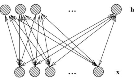
1.1 Undirected graphical model of a Restricted Boltzmann Machine (RBM). There are no links between units of the same layer, only between input (or visible) units xj and hidden units hi, making the conditionals P (h|x) and P (x|h) factorize conveniently. . . . 17
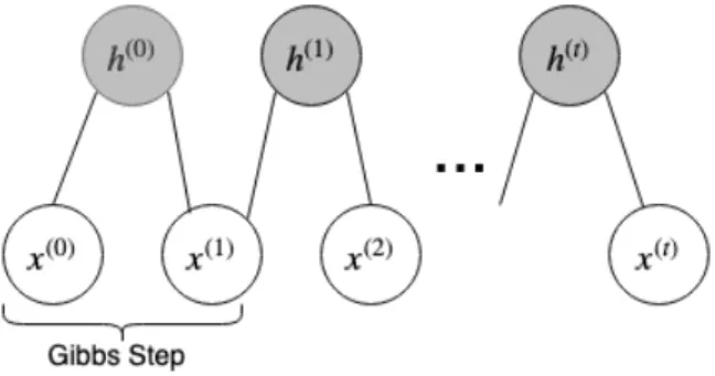
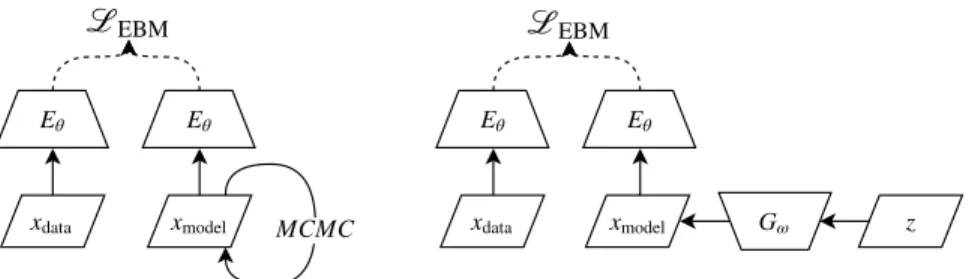
1.2 Illustration of Blocked Gibbs Sampling in RBMs. As t! 1, sample (x(t), h(t)) are guaranteed to be samples of P (x, h) . . . . 18 2.1 Left: Traditional maximum likelihood training of energy-based
mo-dels. Right: Training of maximum entropy generators for energy-based models . . . 28
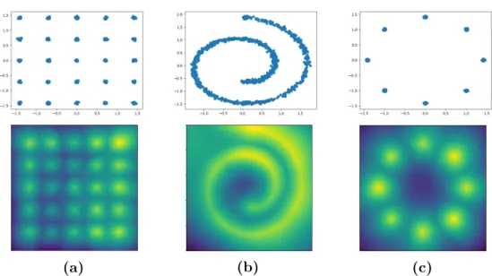
2.2 Top: True data points for three popular toy dataset (a) 25-gaussians, (b) swiss roll, and (c) 8-gaussians. Bottom: Corresponding probabi-lity density visualizations using the learned energy function. Density was estimated using a sample based approximation of the partition function. . . 37
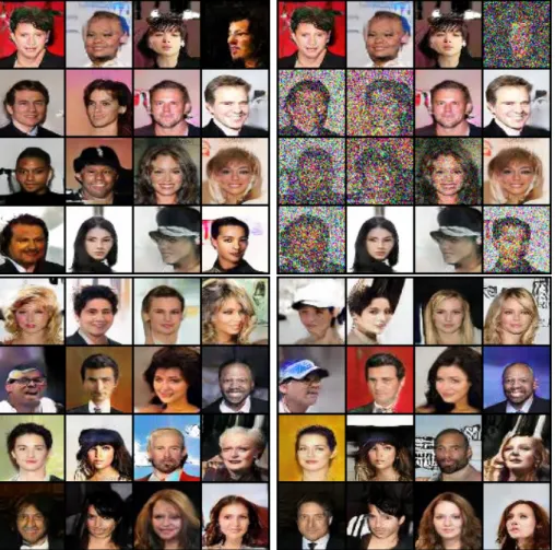
2.3 Samples from the beginning and end of the MCMC in visible space (top) and latent space (bottom) using the MALA proposal and acceptance criteria. MCMC in visible space has poor mixing and gets attracted to spurious modes, while MCMC in latent space seems to change semantic attributes of the image, while not producing spurious modes. . . 42
Liste des tableaux
2.1 Number of captured modes and Kullback-Leibler divergence between the training and samples distributions for ALI [Dumoulin et al., 2016], Unrolled GAN [Metz et al., 2016], VeeGAN [Srivastava et al., 2017], WGAN-GP [Gulrajani et al., 2017]. Numbers except MEG and WGAN-GP are borrowed from Belghazi et al. [2018] . . . 38
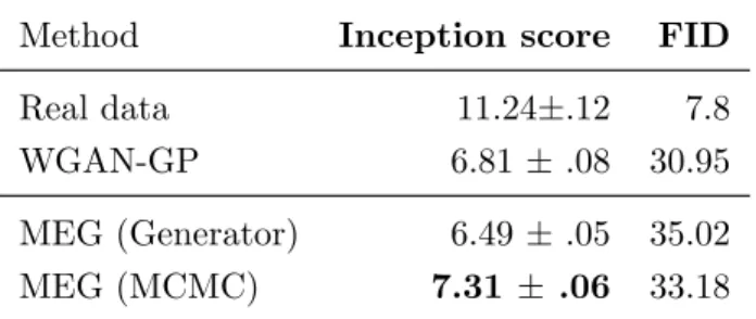
2.2 Inception scores and FIDs with unsupervised image generation on CIFAR-10. We used 50000 sample estimates to compute Inception Score and FID. . . 39
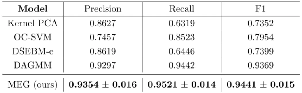
2.3 Performance on the KDD99 dataset. Values for OC-SVM, DSEBM values were obtained from Zong et al. [2018]. Values for MEG are derived from 5 runs. For each individual run, the metrics are averaged over the last 10 epochs. . . 40
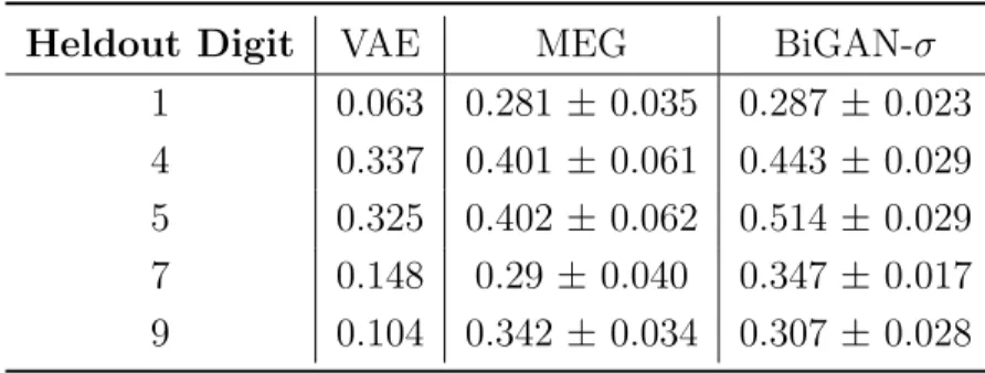
2.4 Performance on the unsupervised anomaly detection task on MNIST measured by area under precision recall curve. Numbers except ours are obtained from [Zenati et al., 2018]. Results for MEG are averaged over the last 10 epochs to account for the variance in scores. . . 41
List of Abbreviations
MEG Maximum Entropy GeneratorsMCMC Markov Chain Monte Carlo GAN Generative Adversarial Networks PCA Principal Components Analyis
t-SNE t-Distributed Stochastic Neighbour Embedding CI Conditional Independence
GM Graphical Model
DGM Directed Graphical Model DAG Directed Acyclic Graph HMM Hidden Markov Model VAE Variational Auto-Encoder UGM Undirected Graphical Model
CPD Conditional Probability Distribution MALA Metropolis Adjusted Langevin Algorithm MH Metropolis Hastings
RBM Restricted Boltzmann Machine WGAN Wasserstein GAN
RNN Recurrent Neural Networks EBM Energy Based Model
CD Contrastive Divergence MI Mutual Information
Acknowledgments
I am extremely grateful for an amazing set of family, friends and advisors without whom my work would not be possible.
I’m grateful to Prof. Yoshua Bengio for accepting me as a graduate student and for encouraging me to explore deep learning research in a variety of disciplines such as speech, vision and natural language processing. His guidance has been instrumental in helping me become the researcher that I am today. I would also like to thank Prof. Aaron Courville for all the helpful research guidance he has provided throughout my study.
I would like to the thank the following co-authors, co-workers, and colleagues (ran-dom order): Kundan Kumar, Kyle Kastner, Soroush Mehri, Jose Sotelo, Alexandre de Br´ebisson, Sandeep Subramanian, Sherjil Ozair, Anirudh Goyal, Tristan Deleu, Shagun Sodhani, Evan Racah, Sai Krishna, Ankesh Anand, Pablo Piantanida, Ales-sandro Sordoni, Philip Bachman, Sarath Chandar, Dmitriy Serdyuk, Alex Lamb, Olexa Bilanuik, Sai Rajeshwar, Philemon Brakel, Shawn Tan, Chinwei Huang, Sina Honari, Anh Nguyen, Kris Sankaran, Florian Golemo, Devansh Arpit, Iulian Serban, Jae Hyun Lim, Faruk Ahmed ; Thank you for all the though-provoking research conversations and brainstorming sessions.
I owe a huge debt of gratitude to Fr´ed´eric Bastien, Simon Lefran¸cois, Ahmed Mamlouk and Quentin Lux for their support and managing the computing infra-structure at the lab.
My graduate life wouldn’t be as easy without the help of C´eline Begin and Linda Peinthi´ere for all their administrative help during my studies.
Finally, the work reported in this thesis would not have been possible without the financial support from: Ubisoft, Google, Samsung, IBM, NSERC, Calcul Quebec, Compute Canada, the Canada Research Chairs and CIFAR.
1
Introduction
1.1
Overview
Machine learning is an important part of modern computer science with im-portant applications across many industries including commerce, finance, logistics, agriculture, and education. Many detailed references exist for deeply understanding machine learning, such as [Bishop, 2006, Hastie et al., 2005, Murphy,2012, Good-fellow et al.,2016].
In this thesis, we present our work - Maximum Entropy Generators for Energy-based Models (MEG), which focuses on advancing the state of art in unsupervised learning and generative modeling. Unsupervised learning is regarded as crucial for artificial intelligence because it promises to take advantage from unlabelled data [Lake et al., 2017]. This work primarily focuses on improving a particular class of algorithms to solve unsupervised learning called energy-based modeling derived from the probabilistic graphical modeling literature. Our work uses deep learning techniques with neural networks to perform function approximation.
This chapter strives to provide an overview of the pre-requisite concepts and terminology required in order to understand the research work presented in this thesis and its important contributions. We begin by first motivating the impor-tance of advancing research in the topics of unsupervised learning and generative modeling. Second, we provide a short introduction to the field of probabilistic gra-phical modeling - which uses graphs to express conditional dependence structure between random variables in a probabilistic model. Third, we discuss Markov Chain Monte Carlo methods, which are a popular class of algorithms for sampling from high-dimensional probability distributions. Next, we discuss a class of methods for performing unsupervised learning called energy-based modeling, which is the
core focus of this thesis. This section also provides a historical perspective on the previous seminal works that serve as an inspiration for the research presented in this thesis. Finally, we explain terminologies and short concepts from recent deep learning literature, such as neural estimators of mutual information, generative adversarial networks and evaluation metrics used for measuring quality of images.
1.2
Contributions
We propose a novel framework for training energy-based models called Maximum Entropy Generators (MEG) to perform unsupervised learning. A key impediment to train based models has been the requirement to sample from the energy-function during maximum likelihood estimation which requires running an expensive Markov Chain Monte Carlo (MCMC) process in each step. In this work, we pro-vide an alternate, fast and efficient method for maximum likelihood training of energy-based models using amortized neural generators and entropy maximization techniques.
We show that the resulting energy function can be successfully used for anomaly detection and strongly outperforms recently published results with energy-based models. We show that MEG generates sharp images (with competitive scores in quantitative evaluation metrics such as Inception and Fr´echet Inception Distance) and does not su↵er from the common mode-mixing issue of many maximum likeli-hood generative models which results in blurry samples.
We also show that our model accurately captures more modes in the data distribution than standard generative adversarial networks (GANs), thereby solving the common mode collapse issue of state of the art GAN-based generative models.
We note that many terms in the above contributions may seem enigmatic to an average reader. We hope that the following sections in the introduction help in resolving the gap in knowledge that is required to understand the remainder of this thesis.
1.3
Unsupervised Learning
The focus of this research work broadly falls under the category of unsupervised learning and generative modeling. This section provides a short introduction to unsupervised learning, which is a sub-field of machine learning that is concerned with learning without labeled data. Since our proposed model - MEG is also a type of generative model, this section also explains the topic of generative modeling and practical use-cases of generative models such as MEG.
Machine learning is typically divided into supervised and unsupervised lear-ning. In predictive or supervised learning, the objective is typically to learn a mapping from inputs x to labels y, given a labeled training datasetD = {(xi, yi)}Ni=1.
The input variables can be any complex structured object such as images, sentences, audio, etc. The corresponding labels can be image categories, positive or negative sentiment of text and speaker identity. If the output labels are categorical, the task is known as classification. If the output labels are continuous, the task is known as regression.
Unsupervised learning is interesting since it is closer to human and animal learning. We are expected to deduce patterns from the sensory input we receive from the physical world. It is also advantageous to not require human experts to label the data. Unsupervised learning also has the potential learn more complex models because there is more information in the input data than just a simple mapping from the input to a single label.
In unsupervised learning, the objective is to discover interesting patterns in the data using only the input dataset. A few common types of unsupervised learning are:
1. Density estimation, in which the task is to recover the the data distribution pdata. Having access to pdata is useful for a variety of purposes, such as
making predictions. Another popular application is anomaly detection. For ex: a credit card company might suspect fraud if a purchase is very unlikely given a model of a customer’s spending habits. Mixture of gaussians is a popular example for density estimation model.
2. Manifold learning, in which the learning algorithm tries to explain the data as lying on a low-dimensional manifold embedded in the original space. A few examples of such models are nonlinear principal components analysis (PCA) and t-distributed stochastic neighbour embedding (t-SNE) [Maaten
and Hinton, 2008].
3. Clustering, in which the task is to discover a set of categories that the data can be divided into neatly. For example: clustering speech data into groups based on the number of speakers. Example of clustering algorithms include k-means clustering and mean-shift clustering.
1.3.1
Generative Modeling
As defined in [Lake et al.,2017], generative modeling is concerned with learning a model that specifies a probability distribution over the data. For instance, in a classification task with examples X and class labels y, a generative model specifies the distribution of data given labels P (X|y), as well as a prior on labels P (y), which can be used for sampling new examples or for classification by using Bayes’ rule to compute P (y|X). A discriminative model in contrast specifies P (y|X) directly, possibly by using a neural network to predict the label for a given data point, and cannot directly be used to sample new examples or to compute other queries regarding the data.
The intuition is that, generative models try to capture how the data was genera-ted in order to perform other downstream tasks such as classification, semi-supervised learning, denoising, matrix completion, structured prediction etc. One important advantage is that generative models do not require human annotated data and labels. A good generative model captures the salient features and underlying factors of variability from a large amount of unsupervised data. Additionally, a generative model provides a mechanism for producing samples from the distribution learned by the model. In contrast, discriminative models do not care about how the data was generated and instead directly categorize the signal.
Some popular examples of generative models are gaussian mixtures models [Titterington et al., 1985], hidden Markov models [Rabiner, 1989], variational
auto-encoders [Kingma and Welling, 2013], generative adversarial networks [Goodfellow et al., 2014a], etc. Popular examples of discriminative models are support vector machines [Cortes and Vapnik, 1995], k-nearest neighbours [Altman,1992], conditio-nal random fields [La↵erty et al., 2001], etc.
Recently, generative models have been utilized for purposes such as representation learning and semi-supervised learning [Radford et al., 2015, Odena et al., 2017,
Salimans et al., 2016], domain adaptation [Ganin et al., 2016, Tzeng et al.,2017], text to image synthesis [Reed et al., 2016], speech recognition [Graves et al.,2013], speech synthesis [Oord et al.,2016], image compression [Theis et al., 2017], super resolution [Ledig et al., 2017], inpainting [Pathak et al., 2016, Yeh et al., 2017], image enhancement [Zhang et al., 2019] , style transfer and texture synthesis [Gatys et al.,2016,Johnson et al.,2016], image-to-image translation [Isola et al.,2017,Zhu et al., 2017], and video generation and prediction [Vondrick et al., 2016].
1.4
Graphical Model
MEG is an energy-based model, which is a type of undirected graphical model, derived from the probabilistic graphical modeling literature. In this section we pro-vide a background on probabilistic modeling using graphs. Specifically, we motivate the use of graphs to express conditional independence structure between random variables, explain graph terminology and discuss two major types of graphical models - directed and undirected. We also show a particular form of undirected graphical models which serves as the foundation for energy-based models.
Probabilistic modeling attempts to answer the core questions of how to com-pactly represent the joint distributions of multiple correlated random variables such as words in a document, pixels in an image, genes in a micro-array, etc [Murphy,
2012]. Related set of questions that are relevant to probabilistic modeling are infer-ring a set of variables given another and inferinfer-ring the parameters of a distribution given a reasonable amount of data.
By the chain rule of probability, we can always represent a joint distribution as follows, using any ordering of the variables:
p(x1:V) = p(x1)p(x2|x1)p(x3|x2, x1)...p(xV|x1:V 1) (1.1)
They key to efficiently represent large joint distributions is to make assumptions about their conditional independences (CI), where two random variables X and Y are conditionally independent given Z (denoted X ? Y |Z) if and only if (i↵) p(X, Y|Z) = p(X|Z)p(Y |Z). A graphical model (GM) is a way to represent a joint distribution by making CI assumptions. In particular, the nodes in the graph represent random variables, and the (lack of) edges represent CI assumptions. Terminology
A graph G = (V, E) consists of a set of nodes or vertices, V = 1, ..., V and a set of edges, E = {(s, t) : s, t 2 V}. A graph can be represented by an adjacency matrix where G(s, t) = 1 is used to denote that s! t is an edge in the graph. If G(s, t) = 1 i↵ G(t, s) = 1, we say that the graph is undirected, otherwise it is directed. It is also assumed that the graph has no self loops, i.e. G(s, s) = 0.
For a directed graph, the parents of a node is the set of all nodes that feed into it: pa(s), {t : G(t, s) = 1}. Correspondingly, the children of a node is the set of all nodes that feed out of it: ch(s), {s : G(t, s) = 1}.
1.4.1
Directed Graphical Models
In directed graphical models (DGMs), probability distributions over the random variables are represented using a directed acyclic graph (DAG). The directed edges are used to represent the conditional independences exhibited by the probability distribution. The key property of DAGs is that the nodes can be ordered such that parents come before children (topological ordering). Given such an order, the ordered Markov property is defined to be the assumption that a node only depends on its immediate parents, not on all predecessors in the ordering, i.e.,
where pa(s) are the parents of the node s and pred(s) are the predecessors of the node s in the ordering.
In general, the joint probability distribution represented by the graph can be written as: p(x1:V) = V Y t=1 p(xt|xpa(t)) (1.3)
where p(xt|xpa(t)) denotes a non-negative function of the variables normalized such
that R p(xt|xpa(t))dxt = 1.
In recent works, directed versions of graphical models have been used to synthesize sensory data through a sampling process which often converts a simple distribution over latent (or hidden) variables1 that models causes in the sensory data, into complex distributions over the data distribution. The hidden variables often represent quantities of interest, such as the identity of the word that someone is currently speaking. The observed variables are what we measure, such as an acoustic waveform. These models can also be used to analyze sensory data by computing the posterior distribution over latent variables given data. An early instantiation of this idea was the Helmholtz machine [Dayan et al., 1995], in which the analysis was performed by a recognition model and the synthesis was performed by a separate generative model, and the two were trained together to maximize the marginal probability of the data. Popular example of directed graphical modeling include the hidden Markov models (HMMs) [Rabiner, 1989] and the more recent work on variational auto-encoders (VAE) [Kingma and Welling, 2013, Rezende et al., 2014].
1.4.2
Undirected Graphical Models
In undirected graphical models (UGMs), also called Markov random fields, the probability distribution over the random variables is represented using an undi-rected graph, which is more natural for certain problems such as image analysis and spatial statistics. From Murphy [2012], UGMs define CI relationships via simple graph separation as follows: for sets of nodes A, B, and C, we say xA?G xB | xC
i↵ C separates A from B in the graph G. This means that, when we remove all
1. In statistics, latent variables (as opposed to observable variables), are variables that are not directly observed but are rather inferred (through a mathematical model) from other variables that are observed (directly measured)[Wikipedia,2019a].
the nodes in C, if there are no paths connecting any node in A to any node in B, then the CI property holds. This is called the global Markov property for UGMs.
The set of nodes that renders a node t conditionally independent of all the other nodes in the graph is called t’s Markov blanket ; denote by mb(t). Formally, the Markov blanket satisfies the following property:
t ? V \ cl(t)|mb(t) (1.4)
where cl(t) , mb(t) [ {t} is the closure of node t. In a UGM, a node’s Markov blanket is its set of immediate neighbours. This is called the undirected local Markov property. From the local Markov property, we can also easily see that two nodes are conditionally independent given the rest if there is no direct edge between them. This is called the pairwise Markov property.
Unlike DGMs which associate a conditional probability distribution (CPD) with each node in the graph (of the form p(xs|xpa(s)), UGMs associate potential
functions or factors with each maximal clique in the graph. The potential function for clique c is given by c(xc|✓c) where ✓c denotes the parameters of the potential
function for clique c. The potential function can be any non-negative function of its arguments. The joint distribution is then defined to be proportional to the product of clique potentials: p(x|✓) = 1 Z(✓) Y c2C c(xc|✓c) (1.5)
where C is the set of all maximal cliques in the graph G and Z(✓) is the partition function given by:
Z(✓),X
x
Y
c2C
c(xc|✓c) (1.6)
Note that the partition function ensures that the overall distributions sums to 1. Hence it is also called the normalization constant.
potential function or clique potential can also be represented as an energy function E(xc) > 0 which denotes the energy associated with the variables in clique c:
c(xc|✓c) = exp( E(xc|✓c)) (1.7)
It can be seen that high probability states correspond to low energy configurations and low probability states correspond to high energy configurations. Models of this form are known as energy based models.
In recent work, these methods model the data as the stationary distribution of a stochastic process (e.g. various Boltzmann machines ; Salakhutdinov and Hinton
[2009]). Sampling under this method corresponds to a potentially powerful iterative process of repeatedly applying a fixed stochastic operator that can gradually turn simple initial distributions over data into complex stationary distributions over data. However a key impediment to this approach is the mixing time problem: if the stationary distribution has multiple modes, the sampling process can take a long time to mix, or reach the stationary distribution, due to the excessive time sampling methods can take to jump between modes.
1.5
Markov Chain Monte Carlo Inference
In this section, we explain the topic of Monte Carlo approximations and also inference using Markov Chain Monte Carlo (MCMC). Monte Carlo approximations are omnipresent in deep learning literature since the optimization of neural networks is typically performed using mini-batch stochastic gradient descent (which uses a stochastic (Monte Carlo) estimate of the true batch gradient across the entire dataset). Additionally, energy-based models such as MEG also use Monte Carlo approximations of the log-likelihood gradient (explained in detail in the energy-based models section).
MCMC is the most popular method for sampling from high-dimensional distri-butions and was placed in the top 10 most important algorithms of the 20th century.
MCMC methods are relevant in the context of energy-based modeling since it is re-quired to sample from the energy-function during the maximum likelihood training of EBMs (explained in detail in the following section). Specifically in our work on MEG, we use a popular MCMC method called Metropolis-adjusted Langevin algorithm (MALA) [Wikipedia,2019b] to generate high quality samples from our energy-model.
In general, Monte Carlo approximations use the principle that computing the distribution of a function f of a random variable X can be expensive to compute using the change of variables formula. Instead, we can approximate the distribution of f (X) using the empirical distribution of the samples {f(xs)}S
s=1,
where x1, ..., xS ⇠ p(X). Thus, we can use Monte Carlo to approximate the expected
value of any function of a random variable as follows:
E[f(X)] ⇡ S1
S
X
s=1
f (xs) (1.8)
However, drawing samples x1, ..., xS ⇠ p(X) might be non-trivial in practical
use-cases when p(X) is a very high-dimensional probability distribution. This motivates the necessity for algorithms that can draw samples from high-dimensional probabi-lity distributions. Markov Chain Monte Carlo is a popular class of algorithms that attempt to solve this problem.
From Murphy [2012], the basic idea behind Markov Chain Monte Carlo is to construct a Markov chain on the state space X whose stationary distribution is the target density p⇤(x) of interest (this may be a prior or a posterior). That is, we perform a random walk on the state space, in such a way that the fraction of time we spend in each state x is proportional to p⇤(x). By drawing (correlated !) samples
x0, x1, x2, ... , from the chain, we can perform Monte Carlo integration wrt p⇤.
1.5.1
Gibbs Sampling
Gibbs sampling is one of the most popular MCMC algorithms and is also the most widely used algorithm for sampling from energy-based models.
conditioned on the values of all the other variables in the distribution. That is, given a joint sample xs of all the variables, we generate a new sample xs+1 by sampling
each component in turn, based on the most recent values of the other variables. An example of a Gibbs sampling step with 3 variables:
xs+11 ⇠ p(x1|xs2, xs3)
xs+1
2 ⇠ p(x2|xs+11 , xs3)
xs+13 ⇠ p(x3|xs+11 , xs+12 )
The expression p(xi|x i) is called the full conditional of the variable i. If p(x) is
represented as a graphical model, the full conditional for variable i will reduce to the Markov blanket of i, which are its neighbours in the graph.
The shortcoming of Gibbs sampling is that it is typically slow and sequential since each Gibbs step requires D steps where D is the number of variables in the graph.
1.5.2
Metropolis Hastings algorithm
Although Gibbs sampling is simple, it is restrictive in terms of the class of models to which it can be applied, such as when the corresponding graphical model has no useful Markov structure. In addition, Gibbs sampling can be slow as men-tioned above. Metropolis Hastings (MH) algorithm is a more general algorithm that can alternatively be used to sample from high-dimensional probability distri-butions. This topic is specifically relevant in context to our work, since we use a variant of the Metropolis Hastings algorithm to draw samples from our energy model.
The basic idea of MH algorithm as defined in Murphy [2012] is, in each step, first a proposal is made to move to a new state x0 from state x with probability
q(x0|x), where q is known as the proposal distribution. Next, the proposal to move
to state x0 is accepted or rejected depending on a formula that ensures that the
fraction of time spent on each state x is proportional to p⇤(x) (necessary since we
want the stationary distribution of the Markov chain to be p⇤(x)). If the proposal is accepted, the new state is x0, else the new state is the same as the current state
x. If the proposal distribution is symmetric, so q(x0|x) = q(x|x0), the acceptance
probability of MH is given by:
r = min 1,p
⇤(x0)
p⇤(x) (1.9)
It can be seen that if x0 is more probable than x, we definitely move there (since
p⇤(x0)
p⇤(x) > 1), but if x0 is less probable, we may still move there anyway, depending
on the relative probabilities. So instead of greedily moving to only more probable states, we occasionally allow ”downhill” moves to less probable states. We direct the reader to [Murphy, 2012] for proof that this procedure ensures that the fraction of time we spend in each state x is proportional to p⇤(x).
If the proposal distribution is asymmetric, i.e q(x0|x) 6= q(x|x0), the Hastings
correction is used to compute the acceptance probability:
r = min(1, ↵) (1.10)
↵ = p
⇤(x0)q(x|x0)
p⇤(x)q(x0|x) (1.11)
Intuitively, it can be seen that this correction is required to fix the bias introduced by the proposal distribution that might itself favor certain states.
The most important reason why MH is a useful algorithm is that, the calculation of the acceptance probability ↵ only requires to know the target density p⇤(x) up
to a normalization constant. For example, supposed p⇤(x) = 1
Zp(x) where Z is the˜
normalization constant, then:
↵ = (˜p(x
0)/Z)q(x|x0)
(˜p(x)/Z)q(x0|x) (1.12)
It can be seen that the Z’s cancel. Therefore we can sample from the target distribution p⇤ even if Z is unknown. This will be especially important to sample
1.6
Energy Based Models
Our work on MEG is primarily an energy-based model. This section provides a background into energy-based modeling. Having provided a short introduction to energy-based models in the previous section on undirected graphical models, we further elucidate the topic in this section followed by a short description of seminal works such as Boltzmann machines and restricted Boltzmann machines (RBMs). We also discuss important impediments in this class of methods to motivate research in this direction and also explain prior attempts at alleviating these shortcomings such as contrastive divergence. We also shortly describe promising alternatives to contrastive divergence such as persistent MCMC and score matching. MEG uses a variant of score matching as one of the objectives to train the energy-function.
Additionally, we revisit the topic of Markov Chain Monte Carlo (MCMC) methods for sampling from EBMs. MCMC sampling is crucial for energy-based modeling since it is required in the training process and also useful for visualizing what the model has learned. Obtaining good samples can be a task of its own as well, for example - the task of unconditional generative modeling of music, speech or images. In this task, the objective is to synthesize new images after learning a model on a dataset of images. Much like standard EBMs, MEG uses MCMC algorithms (specifically, the MALA algorithm) to visualize samples from the energy-function
Energy-based models (EBMs) capture dependencies by associating a scalar value (called energy) to each configuration of the variables of interest [LeCun et al.,2006,LeCun and Huang,2005,Boureau et al.,2007]. Learning corresponds to carving the energy function so that its shape has desirable properties. For example: we would like plausible (observed) configurations to have low energy and unobserved configurations to have high energy. Inference corresponds to clamping the value of the observed variable and finding configurations of the remaining variables that minimize the energy. Loss functional - minimized during learning, is used to measure the quality of the available energy functions.
Probabilistic models must be properly normalized, which may require evaluating intractable integrals over the space of all possible variable configurations. Since
EBMs have no requirement for proper normalization, this problem is naturally circumvented. EBMs therefore provide considerably more flexibility in the design of architectures and training criteria than approaches requiring explicit probability computations.
Energy-based probabilistic models define a probability distribution through an energy function E(x), as follows:
P (x) = e
E(x)
Z , (1.13)
ie., energies operate in the log-probability domain.
The normalization factor Z is called the partition function by analogy with physical systems,
Z =X
x
e E(x) (1.14)
An energy-based model can be learnt by performing (stochastic) gradient descent on the empirical negative log-likelihood of the training data
L(✓, D) = 1 N
X
x(i)2D
log p(x(i)) (1.15)
where @ log p(x@✓ (i)) is the stochastic gradient and ✓ represents the parameters of the energy function.
1.6.1
EBMs with Hidden Units
Usually, we want to introduce some non-observed (latent) variables to increase the expressive power of the model. So we consider an observed part x and a hidden part h: P (x, h) = e E(x,h) Z and P (x) = X h e E(x,h) Z (1.16)
To map to a formulation similar to (1.13), the notation of free energy F(x) is introduced and defined as follows:
P (x) = e F (x) Z where Z = X x e F(x) (1.17) F(x) = logX h e E(x,h) (1.18)
The free energy is just a marginalization of energies in the log-domain. The data log-likelihood gradient then has a particularly interesting form. Starting from (1.17), we obtain: @ log P (x) @✓ = @F (x) @✓ + 1 Z @Z @✓ (1.19) = @F (x) @✓ + 1 P ˜ xe F(˜x) X ˜ x @e F(˜x) @✓ (1.20) = @F (x) @✓ 1 Z X ˜ x e F(˜x)@F(˜x) @✓ (1.21) = @F (x) @✓ X ˜ x P (˜x)@F(˜x) @✓ (1.22)
The average log-likelihood gradient over the training set D is: Ex⇠D @ log P (x) @✓ =Ex⇠D @F(x) @✓ | {z } positive phase Ex⇠P @F(x) @✓ | {z } negative phase (1.23)
The terms positive and negative do not refer to the sign of each term in the equation, but rather reflect their e↵ect on the probability density defined by the model. The first term increases the probability of training data (by reducing the corresponding free energy), while the second term decreases the probability of samples generated by the model.
Therefore, if we could sample from P and compute the free energy tractably, we would have a Monte Carlo method to obtain a stochastic estimator of the log-likelihood gradient. Thus, Markov Chain Monte Carlo (MCMC) methods are very important for energy-based models since the log-likelihood gradient requires
sampling from P.
1.6.2
Boltzmann Machines
The Boltzmann machine is a particular type of energy-based model with hidden variables. The energy function is a general second-order polynomial:
Energy(x, h) = b0x c0h h0W x x0U x h0V h. (1.24) The parameters bi and ci are o↵sets, and Wij, Uij and Vij are weight matrices. The
parameters are collectively denoted ✓.
The gradient of the log-likelihood can be written as: @ log P (x) @✓ = X h P (h|x)@E(x, h) @✓ + X ˜ x,h P (˜x, h)@E(˜x, h) @✓ (1.25)
Similar to (1.23), in the positive phase x is clamped to the observed input vector and we sample h given x ; and in the negative phase both x and h are sampled from the model itself. In general, only approximate sampling can be achieved tractably, by using an iterative procedure that constructs an MCMC. Gibbs sampling, as explained in the previous sections, is a popular MCMC procedure used with RBMs [Hinton et al., 1986, Ackley et al., 1985].
Drawback of general Boltzmann Machines: Since an MCMC chain is required both for the positive phase and the negative phase for each example x, the computation of the gradient can be very expensive, and training time very long.
1.6.3
Restricted Boltzmann Machines
RBMs are undirected probabilistic graphical models containing a layer of obser-vable variables and a single layer of latent variables. RBMs may be stacked (one on top of the other) to form deeper models.
Figure 1.1 – Undirected graphical model of a Restricted Boltzmann Machine (RBM). There are no links between units of the same layer, only between input (or visible) units xj and hidden units
hi, making the conditionals P (h|x) and P (x|h) factorize conveniently.
From Figure 1.1 it can be seen that hi are independent of each other when
conditioning on x and the xj are independent of each other when conditioning on
h (It is a bipartite graph, with no connections permitted between any variables in the observed layer or between any units in the latent layer). Since the graph is bipartite in an RBM, U = 0 and V = 0 from (1.24). i.e., the only interaction terms are between a hidden unit and a visible unit, but not between units of the same layer. As a consequence, the energy function is bilinear:
E(x, h) = b0x c0h h0W x. (1.26) In RBMs, factorization can be utilized to tractably compute the Free Energy and the conditional probabilities P (h|x) and P (x|h) required in the log-likelihood gradient (1.23). Thus: F (x) = b0x X i logX hi ehi(ci+Wix) (1.27) P (h|x) =Y i P (hi|x) (1.28) P (x|h) =Y i P (xi|h) (1.29)
The visible units x and hidden units h are typically modeled as bernoulli or gaussian units. For detailed derivation of the above equations, refer [Bengio,2009].
1.6.4
Sampling in RBMs
Sampling from RBMs is useful for several reasons. First, it is useful in learning algorithms to get a stochastic estimator of the log-likelihood gradient. Second, it is also useful in sampling from the RBMs used as a generative model, or for visual inspection and to get an idea of what the model has captured about the data distribution.
Since RBMs enjoy the factorization introduced by the conditional independence structure, it brings two major benefits: First, we do not have to sample in the positive phase since free energy can be computed in closed form. Second, the set of variables in (x, h) can be sampled in only two sub-steps in each step of the Gibbs chain (as opposed to N sub-steps in Boltzmann machines). First we sample all the hi given x in parallel, and then all the new xj in parallel given h. This type of
Gibbs sampling in general is called Blocked Gibbs Sampling.
Figure 1.2 – Illustration of Blocked Gibbs Sampling in RBMs. As t! 1, sample (x(t), h(t)) are
guaranteed to be samples of P (x, h)
Figure 1.2shows an illustration of t steps of the blocked Gibbs chain for sampling from RBMs. Typically, the chain is seeded using an example from the training set. This makes sense because, as the model captures the training data better, the model distribution and training distribution become more similar. In theory, each parameter update in the learning process would require running one such chain to convergence. This would be computationally expensive. Several algorithms have been devised for RBMs in order to efficiently sample from P (x, h) during the training process.
1.6.5
Contrastive Divergence
Contrastive Divergence is an approximation of the log-likelihood gradient that has been found to be a successful update rule for training RBMs.
The first approximation replaces the average over all possible inputs (second term in (1.23)) by a single example. This is justified since we typically update parameters using stochastic or mini-batch gradient updates. The extra variance introduced from one or few MCMC samples instead of the complete summation might be partially cancelled during the online gradient updates, over consecutive parameter updates. The additional variance introduced by this approximation might not hurt much if it is comparable or smaller than the variance due to online gradient descent.
The second approximation combats the issue of running a long MCMC chain which is expensive. The idea of k-step Contrastive Divergence (CD-k) [Hinton,1999,
2002] is to run the MCMC chain for only k steps (x1, x2, ..., xk+1) starting from the
training example x1 = x. The bias introduced by this approximation vanishes when
k ! 1. However a surprising empirical result was that k = 1 (CD-1) works well [Carreira-Perpinan and Hinton,2005].
An intuitive interpretation of the Contrastive Divergence algorithm is that it approximates the log-likelihood gradient locally around the training example x1.
The stochastic reconstruction ˜x = xk+1(for CD-k) has a distribution centred around
the training point x1 and spreads around as k increases. The CD-k update decreases
the free energy of the training point x1 and increases the free energy of ˜x in the
neighbourhood of x1, thus ”shoveling” energy elsewhere. Thus, the Contrastive
Divergence algorithm is fueled by the contrast between the statistics collected when the input is a real training example and when the input is a chain sample since what is required by a training algorithm for an energy-based model is that it makes the energy of observed inputs smaller, shoveling energy elsewhere, and most importantly in areas of low energy (locally around the training example, here).
1.6.6
Alternative to Contrastive Divergence
Persistent MCMC [Salakhutdinov and Hinton, 2009, Tieleman, 2008b] This idea is to use a background (persistent) MCMC chain to obtain the negative phase samples, instead of running a new short chain as in CD-k. The approximation made is that we ignore the fact that parameters are changing as we move along the chain. However this approximation works very well in practice usually giving rise to better log-likelihood than CD-k probably because the parameters vary slowly during training.
Score Matching [Hyv¨arinen, 2005, Vincent,2011] This is a general approach to energy-based model training in which energy can be computed tractably but not the normalization constant Z. The score function of a density P (x) is = @ log P (x)@x . The basic idea is to match the score function of the model with the score function of the empirical density. This idea exploits the fact that the score function does not depend on the normalization constant.
1.7
Recent Deep Learning Methods
The research work presented in this thesis lies at the intersection of deep learning and energy-based graphical modeling. MEG is an energy-based model that uses deep neural network based function approximators to model the energy-function. Having given a background on graphical models in the previous sections, this section strives to inform the reader about the various concepts popular in the recent deep learning literature. Specifically, we explain the recent methods to estimate mutual informa-tion using neural networks. This concept was instrumental in performing entropy maximization of the energy-function, that arises from the theoretical framework provided by MEG. We also provide a concise description of generative adversarial networks (GANs) [Goodfellow et al.,2014a] since the training of the energy-function in our method draws parallels with the adversarial training of GANs. Further, we also explain some of the evaluation metrics used in our paper for measuring the quality of generated image samples, such as Inception Score (IS) and Fr´echet
Inception Distance (FID).
1.7.1
Neural Estimators of Mutual Information
DefinitionsEntropy is a quantity that measures the unpredictability of a random variable. Entropy of a discrete random variable X with probability mass function (PMF) p(x) is:
H(X) = X
x
p(x) log p(x) = E[log p(x)] (1.30) The entropy measures the expected uncertainty in X.
The di↵erential entropy of a continuous random variable X with support X and probability density function (PDF) f (x) is:
h(X) = Z
f (x) log f (x)dx = E[log(f(x))] (1.31) Mutual information (MI) is a quantity that measures a relationship between two random variables. In particular, it quantifies the ”amount of information” (in units such as Shannons, commonly called bits) obtained about one random variable through observing the other random variable. Mutual information captures non-linear statistical dependencies between variables, and thus can act as a measure of true dependence [Kinney and Atwal, 2014]. Mutual Information quantifies the dependence between random variables X and Z as :
I(X; Z) = Z X⇥Z log dPXZ dPX ⌦ dPZ dPXZ. (1.32)
where PXZ is the joint probability distribution, and PX =
R
ZdPXZ and PZ =
R
XdPXZ are the marginal distributions and ⌦ denotes the Cartesian product.
Mutual information can be equivalently expressed as the Kullback-Leibler diver-gence (KL diverdiver-gence) between the joint and the product of the marginal probability
distributions:
I(X; Z) = DKL(PXZ || PX ⌦ PZ) (1.33)
KL Divergence (KLD) between two discrete probability distributions P and Q defined on the same probability space can be defined as:
DKL(P||Q) = X x2X P (x) log ✓ Q(x) P (x) ◆ (1.34)
Jensen-Shannon Divergence (JSD) is a smoothed and symmetrized version of the KL divergence DKL(P||Q) defined as:
JSD(P||Q) = 1 2DKL(P||M) + 1 2DKL(Q||M), where M = 1 2(P + Q) (1.35) Methods
Mutual Information Neural Estimator (MINE) [Belghazi et al.,2018] uses the the Donsker-Varadhan dual representation of the KL-divergence [Donsker and Varadhan, 1975] to exploit the bound:
I(X; Z) sup
✓2⇥EPXZ
[T✓] log(EPX⌦PZ[e
T✓]). (1.36)
where T✓ :X ⇥ Z ! R is the family of functions parametrized by a neural network
with parameters ✓ 2 ⇥.
DeepInfoMax (DIM) [Hjelm et al.,2018] uses the Jensen-Shannon MI estimator following the recent formulation of f-divergences by [Nowozin et al., 2016]. DIM showed more stable results for MI maximization using the Jensen-Shannon MI estimator, due to its bounded nature. MINE on the other hand leads to an unbounded estimate, rendering it unsuitable for MI maximization without tricks to adaptively clip the gradients during training.
1.7.2
Generative Adversarial Network
Generative Adversarial Network (GAN) [Goodfellow et al.,2014a] is a framework in which two networks - Discriminator (D) and Generator (G) are pitted against each other. The Discriminator attempts to determine whether a sample is from the model distribution or the data distribution. The Generator attempts to ge-nerate samples that are indistinguishable from the original data by the Discriminator.
Formally, let pdata(x) denote the data distribution, pz(z) denote the prior
dis-tribution on the noise variables z and pg denote the Generator’s distribution. The
Discriminator and Generator networks in GANs are trained to optimize the following objective function:
min
G maxD V (D, G) =Ex⇠pdata(x)[log D(x)] +Ez⇠pz(z)[log(1 D(G(z)))]. (1.37)
It has been shown in Goodfellow et al.[2014a] that GANs optimize the Jensen-Shannon divergence (JSD) between the distributions pdata(x) and pg.
Wasserstein GAN
A serious problem with GAN training as noted by [Arjovsky et al., 2017a] and in the original formula [Goodfellow et al., 2014a] is that on complex problems, it is difficult to select a generator that has overlapping support with the data distribution without adding noise. When the generator and the data distribution do not have overlapping support, KL divergence is undefined and the Jensen-Shannon divergence is discontinuous at these points. Wasserstein GAN (WGAN) solves this problem by providing a statistical divergence that is continuous and di↵erentiable even when the supports do not overlap.
[Arjovsky et al.,2017a] thus provides a formulation of the GAN objective which corresponds to optimizing the Earth Mover’s distance or the Wasserstein metric. The Wasserstein distance (or EM distance) can be intuitively thought of as the minimum amount of e↵ort required to move mass distributed according to one distribution to match another distribution. WGAN uses the Kantorovich-Rubinstein
dual formulation for the EM distance: W (Pr,Pg) = sup ||f||L1 ✓ Ex⇠Pr[f (x)] Ex⇠Pg[f (x)] ◆ , (1.38)
where the condition under the supremum indicates that it is over all 1-Lipschitz functions D : X ! R. In practice, the Lipschitz constraint was maintained by clipping the weights within a specific range after each update. [Gulrajani et al.,2017] instead proposed to use a penalty on the norm of the gradient of the discriminator’s output with respect to its inputs. This achieved significantly better results in terms of the quality of samples and training stability over the weight clipping approach.
1.7.3
Evaluation Metrics
In our work, sample quality of generated images is a useful metric to evaluate the generative model. If the model has successfully modeled the data distribution (of images) really well, it should be possible to sample new images that are perceptually consistent and of high quality. Although we can qualitatively evaluate it by visual examination, quantitative metrics are useful to objectively compare competing models. We use two popular methods for this purpose, Inception Score [Salimans et al., 2016] and Fr´echet Inception Distance [Heusel et al., 2017].
Inception Score
From Xu et al. [2018], Inception Score proposed by [Salimans et al.,2016] uses an image classification model M, the Google Inception network [Szegedy et al.,
2016], pre-trained on the ImageNet [Deng et al.,2009] dataset, to compute:
IS(Pg) = exp(Ex⇠Pg[KL(pM(y|x) || pM(y)]) (1.39)
where Pg denotes the generator network’s distribution, pM(y|x) denotes the
label distribution of x as prediction by M and pM(y) = RxpM(y|x)dPg, i.e. the
marginal of pM(y|x) under the probability measure Pg. The expectation and the
integral in pM(y|x) can be approximated with i.i.d samples from Pg.
It can be seen that IS is high when pM(y|x) is close to a point mass, which happens when the Inception network is very confident that the image belongs to a
particular ImageNet category, and pM(y) is close to uniform, i.e. all categories are equally represented. This suggests that the generative model has both high quality and diversity. [Salimans et al., 2016] show that the Inception Score has a reasonable correlation with human judgment of image quality.
Fr´echet Inception Distance
From Borji [2019], FID embeds a set of generated samples into a feature space given by a specific layer of Inception Net (or any CNN). Viewing the embedding layer as a continuous multivariate Gaussian, the mean and covariance are estimated for both the generated data and the real data. The Fr´echet distance between these two Gaussians (a.k.a Wasserstein-2 distance) is then used to quantify the quality of generated samples, i.e
FID(Pr, Pg) =||µr µg||22+ Tr(⌃r+ ⌃g 2(⌃r⌃g)
1
2) (1.40)
where µr, µgand ⌃r, ⌃g represent the mean and covariances of the real and generated
2
Maximum Entropy
Generators for
Energy-based Models
Authors: Rithesh Kumar, Sherjil Ozair, Anirudh Goyal, Aaron Courville and Yoshua Bengio.
This chapter presents a joint work with Sherjil Ozair, Anirudh Goyal, Aaron Courville and Yoshua Bengio. It has been submitted to Neural Information Proces-sing Systems (NeurIPS 2019) - Conference Track.
Contribution: The idea was initially conceptualized by my advisor - Prof. Yoshua Bengio. The idea was further developed and improved by myself through helpful discussions with Anirudh Goyal and Prof. Aaron Courville. I wrote all the code and performed the experiments listed in the paper. Prof. Yoshua Bengio helped write the initial draft of the introduction and background section and Sherjil Ozair helped refine the drafts. I wrote the sections on Maximum Entropy Generators for Energy-based Models (2.3), related work (2.4) and experiments (2.5). I am the first author of the paper.
Affiliation
— Rithesh Kumar, Mila, University of Montreal — Sherjil Ozair, Mila, University of Montreal — Anirudh Goyal, Mila, University of Montreal — Aaron Courville, Mila, University of Montreal — Yoshua Bengio, Mila, University of Montreal
2.1
Introduction
Unsupervised learning promises to take advantage of unlabelled data, and is regarded as crucial for artificial intelligence [Lake et al.,2017]. Energy-based mo-deling (EBMs, LeCun et al. [2006]) is a family of unsupervised learning methods focused on learning an energy function, i.e., an unnormalized log density of the data. This removes the need to make parametric assumptions about the data distri-bution to make the normalizing constant (Z) tractable. However, in practice, due to the very same lack of restrictions, learning high-quality energy-based models is fraught with challenges. To avoid explicitly computing Z or its gradient, Contras-tive Divergence [Hinton, 2000] and Stochastic Maximum Likelihood [Younes, 1998,
Tieleman, 2008a] rely on Markov Chain Monte Carlo (MCMC) to approximately sample from the energy-based model. However, MCMC-based sampling approaches frequently su↵er from long mixing times for high-dimensional data. Thus, training of energy-based models has not remained competitive with other unsupervised learning techniques such as variational auto-encoders [Kingma and Welling, 2014] and generative adversarial networks or GANs [Goodfellow et al., 2014b].
In this work, we propose Maximum Entropy Generators (MEG), a framework in which we train both an energy function and an approximate sampler, which can either be fast (using a generator network G) or uses G to initialize a Markov chain in the latent space of the generator. Training such a generator properly requires entropy maximization of the generator’s output distribution, for which we take advantage of recent advances in nonparametric mutual information maximization [Belghazi et al.,2018, Hjelm et al., 2018,Oord et al., 2018, Poole et al., 2018].
To evaluate the efficacy of the proposed technique, we compare against other state-of-the-art techniques on image generation, accurate mode representation, and anomaly detection. We demonstrate that the proposed technique is able to generate CIFAR-10 samples which are competitive with WGAN-GP [Gulrajani et al., 2017] according to the Fr´echet Inception Distance [Heusel et al., 2017] and Inception Score [Salimans et al.,2016], and is able to generate samples of all the 104 modes of
Figure 2.1 – Left: Traditional maximum likelihood training of energy-based models. Right: Training of maximum entropy generators for energy-based models
We demonstrate that our technique trains energy functions useful for anomaly detection on the KDD99 dataset [Lichman et al.,2013], and that it performs as well as state-of-the-art anomaly detection techniques which were specially designed for the task. Further it vastly outperforms other energy-based and generative models for anomaly detection.
To summarize our contributions, we propose maximum entropy generators (MEG), a novel framework for training energy-based models using amortized neural generators and mutual information maximization. We show that the resulting energy function can be successfully used for anomaly detection, and outperforms recently published results with energy-based models. We show that MEG generates sharp images – with competitive Inception and FID scores – and accurately captures more modes than standard GANs, while not su↵ering from the common mode-mixing issue of many maximum likelihood generative models which results in blurry samples.
2.2
Background
Let x denote a sample in the data space X and E✓ :X ! R an energy function
corresponding to the negative logarithm of an unnormalized estimated density density function
p✓(x) =
e E✓(x)
Z✓ / e
where Z✓ :=
R
e E✓(x)dx is the normalizing constant or partition function. Let p
D be
the training distribution, from which the training set is drawn. Towards optimizing the parameters ✓ of the energy function, the maximum likelihood parameter gradient is @Ex⇠pD[ log p✓(x)] @✓ =Ex⇠pD @E✓(x) @✓ Ex⇠p✓(x) @E✓(x) @✓ (2.2)
where the second term is the gradient of log Z✓, and the sum of the two expectations
is zero when training has converged, with expected energy gradients in the positive phase (under the data pD) matching those under the negative phase (under p✓(x)).
Training thus consists in trying to separate two distributions: the positive phase distribution (associated with the data) and the negative phase distribution (where the model is free-running and generating configurations by itself). This observation has motivated the pre-GAN idea presented by Bengio [2009] that “model samples are negative examples” and a classifier could be used to learn an energy function if it separated the data distribution from the model’s own samples. Shortly after introducing GANs, Goodfellow [2014] also made a similar connection, related to noise-contrastive estimation [Gutmann and Hyvarinen, 2010]. One should also re-cognize the similarity between Eq. 2.2and the objective function for Wasserstein GANs or WGAN [Arjovsky et al.,2017b].
The main challenge in Eq. 2.2 is to obtain samples from the distribution p✓
associated with the energy function E✓. Although having an energy function is
convenient to obtain a score allowing comparison of the relative probability for di↵erent x’s, it is difficult to convert an energy function into a generative process. The commonly studied approaches for this are based on Markov Chain Monte Carlo, in which one iteratively updates a candidate configuration, until these configura-tions converge in distribution to the desired distribution p✓. For the RBM, the most
commonly used algorithms have been Contrastive Divergence [Hinton, 2000] and Stochastic Maximum Likelihood [Younes, 1998, Tieleman, 2008a], relying on the particular structure of the RBM to perform Gibbs sampling. Although these MCMC-based methods are appealing, RBMs (and their deeper form, the deep Boltzmann machine) have not been competitive in recent years compared to autoregressive models [van den Oord et al., 2016], variational auto-encoders [Kingma and Welling,
2014] and generative adversarial networks or GANs [Goodfellow et al., 2014b].
What has been hypothesized as a reason for poorer results obtained with energy-based models trained with an MCMC estimator for the negative phase gradient is that running a Markov chain in data space is fundamentally difficult when the distribution is concentrated (e.g, near manifolds) and has many modes separated by vast areas of low probability. This mixing challenge is discussed by Bengio et al.
[2013] who argue that a Markov chain is very likely to produce only sequences of highly probable configurations: if two modes are far from each other and only local moves are possible (which is typically the case when performing MCMC), it becomes exponentially unlikely to traverse the “desert” of low probability that can separate two modes. This makes mixing between modes difficult in high-dimensional spaces with strong concentration of probability mass in some regions (e.g. corresponding to di↵erent categories) and very low probability elsewhere.
2.3
Maximum Entropy Generators for
Energy-Based Models
We thus propose using an amortized neural sampler to perform fast approximate sampling to train the energy model. We begin by replacing the model distribution p✓ in in Eq.2.2 by a neural generator G parametrized by w. We define PG as the
distribution of the outputs G(z) for z ⇠ pz where pz is a simple prior distribution
such as a standard Normal distribution. @LE @✓ =Ex⇠pD @E✓(x) @✓ Ex⇠pG(x) @E✓(x) @✓ (2.3)
To minimize the approximation error, pG must be close to p✓. To do so, we tune
G to minimize the KL divergence KL(pG||p✓), which can be rewritten in terms of
entropy at the output of the generator:
KL(pG||p✓) = H[pG] EpG[log p✓(x)] (2.4)
= H[pG] + EpG[E✓(x)] + log Z✓ (2.5)
When taking the gradient of KL(pG||p✓) with respect to the parameters w of
the generator, the log-partition function log Z✓ disappears and we can optimize w
by minimizing
LG = H[pG] +Ez⇠pzE✓(G(z)) (2.6)
where pz is the prior distribution of the latent variable of the generator.
In order to approximately maximize the entropy H[pG] at the output of the
generator, we use one recently proposed nonparametric mutual information maxi-mization techniques [Belghazi et al., 2018, Oord et al., 2018, Hjelm et al., 2018].
Poole et al. [2018] show that these techniques can be unified into a single framework derived from the variational bound ofBarber and Agakov[2003]. Since the generator is deterministic, mutual information between inputs and outputs reduces to simply entropy of the outputs, since the conditional entropy of a deterministic function is zero:
I(X, Z) = H(X) H(X|Z) = H(G(Z)) ⇠⇠⇠⇠⇠⇠ ⇠ :0 H(G(Z)|Z)
In particular, we use the estimator from Hjelm et al. [2018], which estimates the Jensen-Shannon divergence between the joint distribution (p(x, z)) and the product of marginals (p(x)p(z)). We refer to this information measure as IJSD(X, Z). We
found that the JSD-based estimator works better in practice than the KL-based estimator (which corresponds to the mutual information).
The estimator of Hjelm et al. [2018] is given by IJSD(X, Z) = sup
T2T Ep(X,Z)
[ sp( T (X, Z))] Ep(X)p(Z)[sp(T (X, Z))] (2.7)
using gradient descent on the parameters of the discriminator T .
With X = G(Z) the output of the generator, IJSD(G(Z), Z) is one of the terms
to be maximized in the objective function for training G, which would maximize the generator’s output entropy H(G(Z)).
Thus the final training objective to be minimized for the generator G and the energy function E is
LG= IJSD(G(Z), Z) +Ez⇠pzE✓(G(z)) (2.8)
LE =Ex⇠pDE✓(x) Ez⇠pzE✓(G(z)) (2.9)
where Z ⇠ pz, the latent prior (typically a N (0, I) Gaussian).
2.3.1
Improving training stability
As can be seen from the above equations, the generator and the energy function are in an adversarial game, similar to generative adversarial networks [Goodfellow et al.,2014b]. This makes optimization via simultaneous gradient descent challenging since the gradient vector field of such an optimization problem is non-conservative as noted by Mescheder et al.[2017]. This is particularly accentuated by the use of deep neural networks for the generator and the energy function. In particular, we no-ticed that during training the magnitude of the energy function values would diverge.
To help alleviate this issue we look towards another technique for learning energy-based models called score matching proposed by Hyv¨arinen [2005]. Score matching estimates the energy function by matching the score functions of the data density and the model density, where the score function is the gradient of the log density with respect to the sample (x) = @ log p(x)@x . If D(x) and E(x) are the
score functions under the data distribution and model distribution respectively, the score matching objective is given by
JSM =Ex⇠PD
⇥
k D(x) E(x)k22
⇤ .
require estimation, Theorem 1 in Hyv¨arinen [2005] shows that with partial integra-tions, the score matching objective can be reduced to the following objective which does not depend on the score function under the data distribution:
JSM =Ex⇠PD X i @i i(x) + 1 2 i(x) 2 =Ex⇠PD X i @2E(x) @2x i +1 2 ✓ @E(x) @xi ◆2 =Ex⇠PD 1 2 @E(x) @x 2 2 +X i @2E(x) @2x i (2.10)
The above objective is hard to optimize when using deep neural networks because of the difficulty in estimating the gradient of the Hessian diagonal, so we use the first term in our objective, i.e. the zero-centered gradient penalty, pushing the data points to sit near critical points (generally a local minimum) of the energy function.
This term is also similar to the gradient penalty regularization proposed by
Gulrajani et al. [2017] which however is one-centered and applied on interpola-tions of the data and model samples, and is derived from the Lipschitz continuity requirements of Wasserstein GANs [Arjovsky et al., 2017b].
2.3.2
Improving sample quality via latent space MCMC
Since MEG simultaneously trains a generator and a valid energy function, we can improve the quality of samples by biasing sampling towards high density regions. Furthermore, doing the MCMC walk in the latent space should be easier than in data space because the transformed data manifold (in latent space) is flatter than in the original observed data space, as initially discussed by Bengio et al. [2013]. The motivation is also similar to that of the “truncation trick” used successfully byBrock et al.[2018]. However, we use an MCMC-based approach for this which is applicable to arbitrary latent distributions.
We use the Metropolis-adjusted Langevin algorithm (MALA, Girolami and Calderhead [2011]), with Langevin dynamics producing a proposal distribution in the latent space as follows:
˜zt+1 = zt ↵
@E✓(G!(zt))
@zt
+ ✏p2⇤ ↵, where ✏ ⇠ N (0, Id)
Next, the proposed ˜zt+1 is accepted or rejected using the Metropolis Hastings
algorithm, by computing the acceptance ratio:
r = p(˜zt+1)q(zt|˜zt+1) p(zt)q(˜zt+1|zt) (2.11) p(˜zt+1) p(zt) = exp E✓(G!(˜zt+1)) + E✓(G!(zt)) (2.12) q(˜zt+1|zt)/ exp ✓ 1 4↵ ˜zt+1 zt+ ↵ @E✓(G!(zt)) @zt 2 2 ◆ (2.13)
and accepting (setting zt+1 = ˜zt+1) with probability r.
The overall training procedure for MEG is detailed in Algorithm 1.
2.4
Related Work
Early work on deep learning relied on unsupervised learning [Hinton et al., 2006,
Bengio et al., 2007, Larochelle et al., 2009] to train energy-based models [LeCun et al., 2006], in particular Restricted Boltzmann Machines, or RBMs. Hinton[2000] proposed k-step Contrastive Divergence (CD-k), to efficiently approximate the ne-gative phase log-likelihood gradient. Subsequent work have improved on CD-k such as Persistent CD [Salakhutdinov and Hinton, 2009, Tieleman, 2008b]. Hyv¨arinen
[2005] proposed an alternative method to train non-normalized graphical models using Score Matching, which does not require computation of the partition function.
Kim and Bengio [2016] and Dai et al. [2017] also learn a generator that approxi-mates samples from an energy-based model. However, their approach for entropy maximization is di↵erent from our own. Kim and Bengio [2016] argue that batch normalization [Io↵e and Szegedy,2015] makes the hidden activations of the generator network approximately Gaussian distributed and thus maximize the log-variance for
![Table 2.1 – Number of captured modes and Kullback-Leibler divergence between the training and samples distributions for ALI [Dumoulin et al., 2016], Unrolled GAN [Metz et al., 2016], VeeGAN [Srivastava et al., 2017], WGAN-GP [Gulrajani et al., 2017]](https://thumb-eu.123doks.com/thumbv2/123doknet/11305980.281697/48.918.238.739.317.494/captured-kullback-divergence-distributions-dumoulin-unrolled-srivastava-gulrajani.webp)