Dynamic Equivalent of a Distribution Grid Hosting Dispersed Photovoltaic Units

(1)

Dynamic Equivalent of a Distribution Grid

Hosting Dispersed Photovoltaic Units

Gilles Chaspierre

Dept. of Elec. Eng. and Comp. Science University of Li`ege, Belgium

g.chaspierre@ulg.ac.be

Patrick Panciatici

Research & Development Dept. RTE, Versailles, France patrick.panciatici@rte-france.com

Thierry Van Cutsem

Fund for Scientific Research (FNRS) University of Li`ege, Belgium

t.vancutsem@ulg.ac.be

Abstract—This paper deals with the derivation of a simplified model of a distribution network hosting dispersed photovoltaic units. The model is aimed at short-term dynamic simulations of a transmission grid in response to large disturbances. In a first step, a generic dynamic model of a photovoltaic unit is proposed, focusing on its interactions with the grid, in particular the controls triggered by voltage disturbances. The model takes into account various present and near-future grid codes. In a second step, a dynamic equivalent is derived accounting for the distribution network, the dispersed photovoltaic units, as well as static and dynamic (motor) loads. This equivalent is of the “grey-box” type and its parameters are tuned in the least-square sense to match the dynamic response of the original, unreduced system. Simulation results are reported on a detailed 913-bus distribution system subject to faults at transmission level.

Index Terms—active distribution networks, photovoltaic units, motor loads, short-term dynamics, dynamic equivalents

I. INTRODUCTION

Power systems are getting increasingly complex because of the fast growing share in the electricity production mix of distributed generation. The latter is mainly connected to distribution grids, and distribution systems will become more and more “active”.

The dynamics of the future power systems will thus arise from many distributed components. Hence, it becomes urgent to account for the contributions of such Active Distribution Networks (ADNs) in power system dynamic studies.

One approach could be the simulation of the combined transmission and distribution systems. In spite of advances in computational power and large-scale simulation algorithms, including parallel processing techniques [1], handling the en-tire, detailed model with hundreds of thousands of differential and algebraic equations is extremely challenging.

Another obstacle could be the confidentiality of data. While the Distribution System Operator (DSO) of a Medium-Voltage (MV) and Low-Voltage (LV) grid is usually entitled to collect data about the connected equipment, sharing this information with the Transmission System Operator (TSO) may raise legal issues.

Finally, collecting all the parameters and matching the operating point of concern may represent a prohibitive data processing problem for the TSO.

Clearly it makes sense for the DSOs to process the data of their own systems and transmit to the TSO reduced,

“anonymized” models of significantly lower complexity than the original, unreduced model that they have assembled. Those equivalents are intended to be attached to the model of the transmission system for use by the TSO in dynamic security assessment studies.

This paper focuses on the specific but common case of a distribution grid hosting many PhotoVoltaic (PV) units, at both the MV and LV levels. Nevertheless, the methodology is expected to apply to other power-electronics interfaced generators.

The dynamic model and its equivalent are derived under the following assumptions: (i) the three-phase distribution grid is assumed to be balanced; (ii) the model is intended for dynamic simulations under the phasor approximation [2], and (iii) emphasis is put on responses to transmission voltage magnitude disturbances.

The rest of the paper is organized as follows. The generic PV unit model adopted in this work is described in Section II. In Section III the test system is presented. Illustrative examples of the model performance are given in Section IV. The deriva-tion of the ADN equivalent is presented in Secderiva-tion V, and the corresponding simulation results are reported in Section VI. Concluding remarks are offered in Section VII.

II. GENERIC MODEL OF APVUNIT AND ITS CONTROLS

The generic model of a PV unit (an upgraded version of the one in [3]) is shown in block-diagram form in Fig. 1.

The model focuses on the interactions of the PV unit with the grid, rather than on a detailed representation of its components. Furthermore, the embedded controls meet the requirements of recent and near-future grid codes for PV units such as those described in Refs. [4], [5], [6] and [7]. The model is parametrized to easily accommodate a specific grid code [8].

In Figure 1, vx and vy are the projections on orthogonal

reference axes (x, y) of the phasor of the terminal voltage. ix

and iy are the corresponding projections of the phasor of the

current injected into the network.

The main parts of the model are described in the rest of

this section. Most of them rely on the measured voltage Vm

which differs from the terminal voltage: Vt=

q v2

x+ vy2

(2)

Over Voltage Protection 1 1 + sTm N D Vt Vm Voltage Support (see Fig. 3) Fvh Fvl IP max 0 1 1 + sTg 1 1 + sTg iP iQ IQmax IQmin Limit updating: see Eqs. (4, 5) 0.01 Fvh Fvl MAX

i

x

i

y 1 s

v

x

v

_y vq _θ iQsup + + IQref Pext 0 Pf lag 1 1 1 + sTm 1 1 + sTm vxm vym kP LL max(di/dt) FP LL 1 0 N D PLL Active -reactive priority iP cmd iQcmd Vm> VP LL Vm< VP LL Vm> VS1 Vm< VS1 LVRT (see Fig. 2)

Reactive current injection

r v2 x+ vy2 vq= vymcos θ − vxmsin θ ix= iPcos θ + iQsin θ iy= iPsin θ − iQcos θ Active current injection

Fig. 1. PV unit generic model (not shown: active power modulation in response to frequency deviation and reactive power absorption in response to overvoltage)

A. Phase Locked Loop controller

The Phase Locked Loop (PLL) controller model is shown at the top of Fig. 1. It ensures that the phasor of the current injected by the PV unit has the proper magnitude and phase angle with respect to the terminal voltage phasor.

With reference to Fig. 2, the PLL controller aims at aligning

its d axis with the measured voltage phasor ¯Vm. θ is the angle between respectively the d axis and the reference x. In steady state, the integrator forces vq = 0; then, θ coincides with the

“true” voltage phase angle θr and vd is equal to the voltage

magnitude.

(3)

y x ¯ Vm vym vxm d q vd vq θ θr ¯ I iq id id= iP iq= −iQ

Fig. 2. Phasor diagram illustrating the PLL principle

1 Vint Vmin 0 T1 T2 Vr V (pu) t(s) Tint V (pu)

Fig. 3. Parametrized LVRT curve (fault occurring at t = 0)

iQ, are obtained from the controls detailed next. In steady

state, when θ coincides with the phase angle of the voltage phasor, iP (resp. iQ) is the active (resp. reactive) current truly injected into the grid.

The speed of response of the PLL can be adjusted through the gain kP LL.

If the terminal voltage is severely depressed and Vm drops

below the threshold VP LL, the PLL is temporarily “frozen”

to avoid instability [9]. This is obtained by switching FP LL

from one to zero (see Fig. 1). B. Low Voltage Ride-Through (LVRT)

An important feature of PV units is their LVRT capability, requiring them to remain connected to the grid during a fault as long as the voltage is above a reference curve, as shown in Fig. 3. This curve can be adjusted by modifying the six parameters T1, Tint, T2, Vmin, Vint and Vr.

The unit disconnection is modeled by the variable Fvl

switching from one to zero. C. Active current injection

The solar irradiation is assumed constant over the simulation interval (of a few seconds), leading to a constant power Pext. Dividing the latter by the voltage Vmand limiting the result to IP max discussed in the sequel yields the active current

command iP cmd.

The inverter response to the iP cmdcommand is represented

by a simple lag block with time constant Tg and an internal

rate limiter. Vm(p.u.) iQsup Dead Band m · Inom kRCI 0 kRCA VS1 VS2 −n · Inom

Fig. 4. Parametrized reactive current injection

D. Reactive current injection

Units may be requested to inject reactive current into the grid in order to support the terminal voltage. As shown in Fig. 4, the injected reactive current varies with the measured voltage according to:

if Vm≤ VS1: iQsup = kRCI(VS1− Vm) + m Inom (1)

if Vm> VS2: iQsup = kRCA(VS2− Vm) − n Inom (2)

else : iQsup = 0. (3)

where Inom is the inverter nominal current. The parameters

m, kRCI, VS1, n, kRCA and VS2 allow changing the

charac-teristics of voltage support, or even disabling this service (for instance, for units connected to an LV grid).

Note that, according to Eq. (2), in case of overvoltage, a reactive current is drawn from the grid (i.e. the unit absorbs reactive power) to alleviate the terminal voltage rise. This mode of operation is not shown in Fig. 1 to preserve legibility.

The component IQref (see Fig.1) is added to the reactive

current setting to comply with some grid codes requiring a nonzero reactive power in steady state.

Again, the inverter response to the iQcmd command is

represented by a lag block with time constant Tg.

E. Active - reactive priority

For efficient voltage support, units are assumed to give priority to reactive current injection during a fault. This may require reducing the active current in order to avoid exceeding

the inverter current limit Inom. The maximum active and

reactive currents are thus given by: IP max = Pf lagInom+ (1 − Pf lag)

q I2 nom− i2Qcmd (4) IQmax = Pf lag q I2

nom− i2P cmd+ (1 − Pf lag)Inom (5) In normal operating conditions, i.e. when VS1< Vm< VS2,

priority is given to active current and the variable Pf lag

is at one. In that case, the maximum value of the active

current (IP max) is set to Inom and the maximum value of

the reactive current (IQmax) depends on the active current

command iP cmd. When the voltage falls below VS1, priority

is given to reactive current, Pf lag switches to zero, IQmax is

(4)

F. Overvoltage protection

When Vm exceeds a high voltage threshold, the unit is

assumed to trip without delay to avoid damaging insulation materials and electronic components.

The unit disconnection is modeled by the variable Fvh

switching from one to zero.

G. Other controls

The model also includes control blocks responding to fre-quency deviations but they are not shown here for clarity, since frequency disturbances are not investigated in this paper.

III. TEST SYSTEM

A. Distribution grid

The 75-bus 11-kV distribution grid previously considered in [3], [10] has been used in this study. Its one-line diagram is shown in Fig. 5. Among the 75 MV buses, it is assumed that 38 feed LV distribution grids to which small residential PV units are connected, as detailed in Section III-B. At the remaining 37 buses, an industrial load and a large PV unit are connected, as detailed in Section III-C.

The total load is 21.9 MW/ 5.4 Mvar for a total PV generation of 11.1 MW, leading to a 11.4 MW/ 7.0 Mvar injection by the HV/MV transformer.

Fig. 5. One-line diagram of the 75-bus 11-kV distribution system

B. LV distribution feeders hosting small PV units

A generic, double LV distribution feeder is connected to some of the MV buses through an MV/LV distribution trans-former, as shown in Fig. 6. The residential loads connected to the LV nodes are represented by an exponential model for the static part, in parallel with a small induction motor for the dynamic part. The motor parameters are taken from [11]. Moreover, a small residential PV unit of a few kW is connected in parallel with each LV load. Those units do not support grid voltages; instead, they trip whenever the terminal voltage magnitude falls below the LVRT curve shown in Fig. 7.a.

11 kV M M M M M M M M M M M M M M M M M M M M 0.4 kV

Fig. 6. LV distribution feeders hosting small residential PV units

1 0.5 0.2 0 0.3 1.5 0.9 V (pu) t(s) 0.7 1 0 1.5 0.9 t(s) 0.8 V (pu) (a) (b)

Fig. 7. LVRT characteristics of: (a) small residential PV units, and (b) large industrial PV units (fault occurring at t = 0)

In terms of installed capacity, all residential PV units together account for 2 MW.

C. Industrial loads with large PV units

Larger, industrial loads and larger PV units are connected to the other buses of the MV grid, as shown in Fig. 8. The loads also include a static part with exponential model and an equiv-alent induction motor, whose parameters are representative of large industrial motors [11]. Those industrial PV units have capacities around a few hundred kW. Hence, they are assumed to have LVRT capability and support the network voltages by injecting reactive current. The corresponding characteristics are shown in Figs. 7.b and 9, respectively.

The durations in this LVRT characteristic are strongly dependent on the protection philosophy of the transmission

network. Moreover, the lowest voltage Vmin= 0.2 pu depends

on the residual voltage magnitudes experienced by the MV grid when faults occur in the transmission system.

In terms of installed capacity, all industrial PV units account for 15 MW.

(5)

PV

M 11 kV

0.4 kV

Fig. 8. Industrial load in parallel with a large PV unit

Vm(p.u.) iQsup

0.2 · Inom

0 0.9

4

Fig. 9. Reactive current injection by large PV units (corresponds to the low voltage part of Fig. 4)

D. Randomization of data

To account for the diversity of loads and PV units in a real-life system, some parameters have been randomly varied around typical values from one bus to another. This is the case for the PV unit installed capacities, the nominal power and the electrical parameters of all induction motors.

E. Overall model complexity

Time simulations have been performed with RAMSES, a software for phasor-mode time simulation developed at the Univ. of Li`ege [12].

The complete system model includes 913 (MV and LV) buses, 797 static loads, 797 induction motors, 37 large PV units, and 760 small PV units.

Each motor is represented with a single-cage model involv-ing 10 differential-algebraic equations. Each PV unit model (see Fig. 1) involves 93 differential-algebraic equations. For simplicity all PLL controllers were tuned identically.

IV. ILLUSTRATIVE EXAMPLES OF MODEL PERFORMANCE

A single operating point of the test system has been consid-ered. Since the simulations last for a few seconds, the active power available on PV units and the load demand are assumed to remain constant.

A. Behaviour of an individual PV unit

A short-circuit taking place at t = 0.1 s and lasting for 100 ms has been applied at some electrical distance of a large industrial PV installation.

Figure 10 shows the time evolution of the active and reactive currents injected into the grid. The unit operates initially at unity power factor. In accordance with the reactive current priority, the PV unit injects reactive current during the fault in order to support the terminal voltage, while the active current

0 0.05 0.1 0.15 0.2 0.25 0.3 0.35 0.4 0.45 0.5 0 0.2 0.4 0.6 0.8 1 (pu) Time (s) Active Current Reactive Current

Fig. 10. Active and reactive current injected by the PV unit before, during, and after a short circuit

0.2 0.3 0.4 0.5 0.6 0.7 0.8 0.9 1 0 0.2 0.4 0.6 0.8 1 1.2 1.4 V (pu) Time (s)

Without grid requirements With grid requirements

Fig. 11. Terminal voltage of the PV unit in the scenario of Fig. 10, with and without reactive current injection and LVRT capability

is strongly reduced in order to not exceed the maximum current of the inverter.

Figure 11 shows the time evolution of the terminal voltage. The response shown with dashed line has been obtained assuming that the unit has LVRT capability and participates to voltage support through reactive current injection. For compar-ison purposes, the response shown with solid line corresponds to the case when the PV unit does not inject reactive current, but trips when the voltage falls below 0.8 pu. As expected, the combined LVRT capability and reactive current injection boosts the voltage recovery significantly. The corresponding effect on the speed of a large industrial motor is shown in Fig. 12. The grid support by the PV unit allows a faster speed recovery (at the cost, however, of some oscillations).

B. System-wide behaviour

The following simulation results show the evolution of voltages in response to various voltage dips applied on the primary side of the HV/MV transformer.

Voltage dips are characterized by their depth, which de-pends on the fault location in the transmission network, and their duration, which relates to protection performances. The following scenarios (inspired of protection design used by one TSO) have been considered:

1) a fault on the transmission grid causing a drop of 0.8 pu, cleared by primary protections after 100 ms;

(6)

0.97 0.975 0.98 0.985 0.99 0.995 1 0 0.2 0.4 0.6 0.8 1 1.2 1.4 Omega (pu) Time (s)

Without grid requirements With grid requirements

Fig. 12. Speed response of a large motor in the scenario of Fig. 10, with and without reactive current injection and LVRT capability

2) a fault on the transmission grid causing a drop of 0.8 pu, cleared by back-up protections after 250 ms;

3) a fault closer to the HV/MV transformer resulting in a drop of 0.95 pu, also cleared after 250 ms. This pes-simistic scenario has been chosen in order to challenge the PV unit grid requirements.

The terminal voltages of a sample of large PV units are shown in Figs. 13, 14 and 15, respectively, corresponding to the three scenarios. In all three cases, the very first voltage drop is significantly smaller than the initiating HV voltage drop, thanks to reactive current injection. However, in Sce-narios 2 and 3, with the fault lasting 250 ms, the voltages eventually drop more significantly than in Scenario 1, with a 100 ms fault duration. This is caused by motor deceleration lasting longer, resulting in high currents and large reactive powers drawn from the grid.

It can also be seen that the LVRT and reactive current injection requirements have been properly specified to avoid unit disconnection in Scenarios 1 and 2. On the other hand, in Scenario 3, almost all PV units terminal voltages drop below the LVRT limit. However, this takes place at the very end of the fault-on period. Under the effect of the measurement

time constant Tm, some units do not detect the LVRT curve

crossing, and remain connected. Out of the 37 large PV units, 11 trip, which represents 25 % of the corresponding active power generation. Furthermore, voltage recovery after fault clearing is significantly slower in Scenario 3 than in Scenario 2.

V. DERIVING THEADNEQUIVALENT

A. Brief literature review

Recent works resort to various techniques in order to derive ADN models. A detailed classification of methods is offered in [13] and [14], for instance. Two main groups of methods are distinguished.

The “conventional” approaches address more specifically the identification of a reduced-order model. They include basically the coherency and the modal analysis methods. The former are based on the identification and aggregation of coherent synchronous generators. Hence, they can hardly

0 0.2 0.4 0.6 0.8 1 0 0.5 1 1.5 2 V(pu) Time (s) HV voltage dip LVRT

Fig. 13. Scenario 1: PV unit voltages vs. HV voltage dip and LVRT characteristic 0 0.2 0.4 0.6 0.8 1 0 0.5 1 1.5 2 V(pu) Time (s) HV voltage dip LVRT

Fig. 14. Scenario 2: PV unit voltages vs. HV voltage dip and LVRT characteristic

be applied to components interfaced to the grid with power electronics. The latter methods are based on state space models linearized around an equilibrium point. For instance, in Ref. [15] the Hankel Norm Approximation has been used for the model reduction of a power system with photovoltaic generation. The results indicate that this method can signif-icantly reduce the model order and simulation times while retaining a good accuracy. However, this is only valid for small deviations from a given operating point. Those approaches are not likely to capture the nonlinear and discontinuous behaviour of distributed generation in response to large disturbances in the transmission system, such as switching from active to reactive current priority, tripping of some units, etc.

In “measurement-based” and “simulation-based” methods, the distribution system response is either measured or sim-ulated and curve fitting techniques are used to determine the model parameters. The methods of this family appear attractive since they can deal with non-synchronous generators and large disturbances.

Among them, the “grey-box” approach, as defined and recommended in [16], is appealing from an engineering viewpoint. The model has a known structure but unknown parameters, to be identified from simulations or measurements. In contrast, a “white-box” model would involve a detailed model of all components. (This corresponds to the unreduced,

(7)

0 0.2 0.4 0.6 0.8 1 0 0.5 1 1.5 2 V(pu) Time (s) HV voltage dip LVRT

Fig. 15. Scenario 3: PV unit voltages vs. HV voltage dip and LVRT characteristic M Equivalent large PV unit Equivalent motor Equivalent exponential load RP V XP V RLoad XLoad Rpv Xpv Equivalent residential PV unit

Fig. 16. Structure of the ADN equivalent

reference model presented in § III.) On the opposite, in a “black-box” approach, the structure of the model is not known a priori. The model can be determined using recurrent Artificial Neural Network, for example [17]. Though, large data sets are required to be informative enough [14]. A major advantage of grey-box models is the ability to embed physical knowledge about the system in the structure of the equivalent. As an example, a “grey-box” generic model of ADN is presented and validated in [18] and [19]. Nevertheless, the original ADN model appears to be relatively small and it is not clear whether the equivalent is able to account for the discrete events triggered by inverter controls in response to large disturbances.

B. Structure of the equivalent

In the spirit of a grey-box approach, the equivalent con-sidered in this work consists of “lumping” various PV units into a single equivalent, represented by the generic model of Section II. Furthermore the PV units are clustered according to the grid requirements they follow. Namely, one equivalent PV generator accounts for the small residential PV units not providing grid support and another one for the large, grid-supporting PV units.

Similarly, all loads are lumped into an equivalent including, for the dynamic part, a 3rd-order induction motor model and,

for the static part, an exponential model:

P = Po( V Vo )α and Q = Qo( V Vo )β (6)

The resulting structure of the equivalent is shown in Fig. 16. To account for voltage drops inside the distribution network, the lumped load and the lumped PV units are in series with equivalent impedances. Separate branches have been consid-ered to avoid the load and the PV units to be all at the same voltage. The six parameters Rpv, Xpv, RP V, XP V, RLoadand

XLoad have to be identified. Note that the model is intended

to be connected on the MV side of the HV/MV transformer, which serves as natural interface with the transmission system (where faults are going to be considered).

C. Partial tripping of equivalent PV unit

As illustrated by the simulation results in Section IV, the equivalent PV units must account for the tripping of some of the individual units they replace. This is a challenging modelling issue because individual units are now lumped into

a single equivalent, with a single terminal voltage Vm. The

problem has been tackled by providing the equivalent PV unit with a “partial tripping” feature as explained next.

Let us define tf as the time during which the terminal

voltage Vm stays below the Vr threshold defined in Fig. 3.

Partial tripping is reflected by multiplying the unit output current by:

F = f1f2f3 with 0 ≤ f1, f2, f3≤ 1

where f1, f2and f3relate to the three time intervals considered hereafter (symbols are defined in Fig. 3).

1) 1st case: tf ≤ T1: f1 varies with Vm as shown in

Fig. 17.a, where 0 ≤ c, d ≤ 1. It is assumed that a fraction

1 − c of the units trips as soon as Vm drops below Vmin,

while the remaining units are progressively disconnected as

Vmfurther drops, as shown by the inclined part of the curve.

f1 Vm Vmin c 1 d Vmin f2 Vm Vint e 1 f Vint (a) tf≤ T1 (b) T1≤ tf≤ Tint f3 1 u T2 tf Tint (c) tf≥ Tint

(8)

2) 2nd case: T1 < tf ≤ Tint: In this case, tripping will

take place if Vm < Vint. The factor f2 varies with Vm

as shown in Fig. 17.b, similar to Fig. 17.a, but with Vint

substituted to Vmin and (e, f ) to (c, d).

3) 3rd case: Tint < tf: In post-fault conditions,

trip-ping may take place due to slow voltage recovery. This is

reflected by f3 which decreases linearly with tf − Tint as

shown in Fig. 17.c, involving the additional parameter u, with Tint/T2< u ≤ 1.

f1, f2 and f3 remain constant after the voltage Vm has

recovered above Vr, considering that the PV units are not

reconnected.

The above model involves five parameters (c, d, e, f and u) to be identified.

Since the simpler LVRT characteristic of Fig. 7.a is used for small PV units, a simplified partial tripping is considered in the corresponding equivalent. It only involves the multiplier

f1 with the two associated parameters c and d.

D. Identifying the parameters of the equivalent

The equivalent ADN involves a total of 39 parameters, as detailed in Table I.

All these parameters are grouped in a θ vector which is adjusted to minimize in the least-square sense the difference between the response of the unreduced and the equivalent systems, respectively. The response is measured in terms of active and reactive powers flowing out of the HV/MV transformer.

The parameters are obtained by applying m distinct training input signals to the models. For the j-th signal (j = 1, . . . , m), we denote by:

Pe(θ, j, k) the discrete-time evolution of the active power

flowing into the equivalent system;

Qe(θ, j, k) the corresponding evolution of reactive power;

Pd(j, k) the discrete-time evolution of the active power

flowing into the unreduced system;

Qd(j, k) the corresponding evolution of reactive power,

where k refers to the discrete times used by the time-simulation solver. The same time instants are considered for both the unreduced and the equivalent system; if needed, interpolation is used to make the time instants coincide. The number of discrete times is denoted by n.

The least-square parameter estimation minimizes:

ε(θ) = εP(θ) + w εQ(θ) (7) where: εP(θ) = m X j=1 αj n n X k=1 [Pe(θ, j, k) − Pd(j, k)]2 (8) εQ(θ) = m X j=1 αj n n X k=1 [Qe(θ, j, k) − Qd(j, k)]2 (9)

under the constraints:

θL≤ θ ≤ θU_.

(10)

The factor w allows adjusting the weight given to the active

power response compared to the reactive one, while the αj’s

allow assigning weights to the various system responses.

θL and θU are vectors of lower and upper bounds on θ,

respectively.

E. Optimization method

Pe(θ, j, k) and Qe(θ, j, k) being obtained from time simu-lation, it is hopeless to derive an analytical expression of the first-order, and even less the second-order, derivatives of ε(θ) with respect to θ. Hence, standard constrained least-square methods can hardly be used unless the above derivatives are estimated numerically.

At this stage, a meta-heuristic global optimization method has been preferred. Meta-heuristic methods provide adaptive rules that tailor the search to the particular landscape of the objective function without specific parameter tuning [20]. More precisely, an Evolutionary Algorithm (EA) has been used to solve the above optimization problem. EA algorithms resort to stochastic rules that allow handling complex high-dimensional problems. To this purpose, at each generation of the EA, a whole population of points is improved rather than a single solution. The Differential Evolution (DE) variant

presented in [21] has been implemented in MATLAB using

the open-source code from [22]. This choice was motivated by the comparison of algorithms reported in [23], based on various benchmark problems, from which DE seems to generally outperform other EA as well as particle swarm algorithms. More precisely, the local-to-best strategy has been chosen since it attempts a balance between robustness and fast convergence [22]. Furthermore, at each new generation, the mutation factor F of the algorithm (see [21]) is randomly selected in the range [0.5, 1.0]. It has been found that this technique may improve convergence significantly.

VI. SIMULATION RESULTS OF THEADNEQUIVALENT

A. Training signals

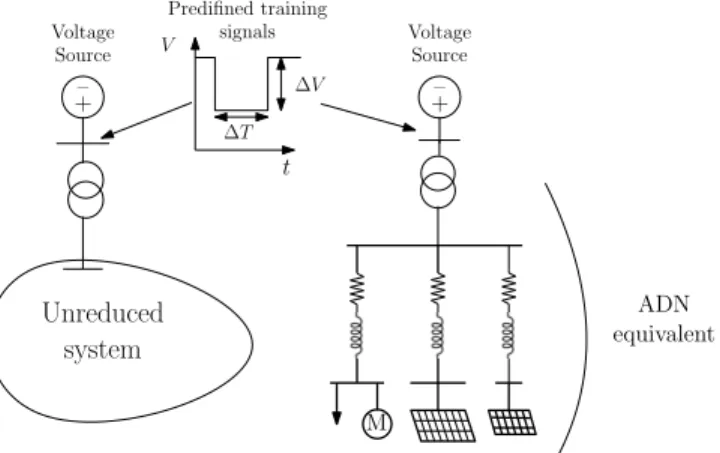
For training purposes, predefined voltage disturbances are applied directly on the HV side of the distribution transformer, as shown in Fig. 18. These signals are characterized by a volt-age drop ∆V and a sag duration ∆T . As already mentioned, the depth and duration of the voltage disturbances depend on the fault location and protection performances, respectively. In this respect, it has been assumed that faults affecting the transmission grid are cleared after either 0.10 or 0.25 s (typical response times of primary and back-up protections), while the voltage drop has been varied from 0.5 to 0.8 pu.

B. Preliminary sensitivity analysis

In a first step, θ has been estimated using a single training signal, characterized by ∆V = 0.6 pu and ∆T = 0.10 s, and a sensitivity analysis has been performed, by varying each parameter individually around that first solution, in order to identify those with little influence.

For instance, for a 100 % variation of each parameter, it was found that only two of them were impacting the error ε(θ) by

(9)

TABLE I

PARAMETERS OF THEADNEQUIVALENT

Type Nb. of parameters

Generic PV model accounting for small PV units

Nominal current Inom 1

Time constants Tmand Tg 2

Parameters c and d of the partial tripping model 2 Series resistance Rpv and reactance Xpv 2

Generic PV model accounting for large PV units

Nominal current Inom 1

Voltages Vmin, Vintand Vrof the LVRT curve 3

Parameters m, kRCIand VS1of reactive current injection 3

Time constants Tmand Tg 2

Parameters c, d, e, f and u of the partial tripping model 5 Series resistance RP V and reactance XP V 2

Equivalent load

Exponents α and β of static load component 2 Static and dynamic parameters of motor component of load 8 Series resistance RLoadand reactance XLoad 2

Share of the initial active and reactive powers by the various components Fraction of total active power produced by equivalent representing large PV units 1 Fraction of total active power produced by equivalent representing small PV units 1 Part of the total active power consumed by static load component 1 Part of the total reactive power consumed by static load component 1

Unreduced system – + ∆V ∆T t V Voltage Source Predifined training signals – + Voltage Source ADN equivalent M

Fig. 18. Training phase using predefined voltage signals

less than 1 %. (One was relative to the motor mechanical torque, and the other was the u parameter in Fig. 17.c.) This very low number suggests that the initial set of parameters had been properly selected. Those two parameters were set to an average value and removed from θ.

C. Training phase

The eight training signals (m = 8) detailed in Table II have been used altogether to estimate θ. All responses have been given the same weight, i.e. w = 1 and αj = 1, j = 1, . . . , 8. A sample of results is given in Figs. 19 - 24, showing the active and reactive power responses of both the detailed and the reduced systems, for the training signals No. 3, 4 and 6. These are the powers entering the HV/MV transformer, on its HV side.

TABLE II

TRAINING SIGNAL CHARACTERISTICS

No ∆V (pu) ∆T (ms) 1 0.5 0.10 2 0.5 250 3 0.6 100 4 0.6 250 5 0.7 100 6 0.7 250 7 0.8 100 8 0.8 250

It is observed that the final active power is slightly larger than the initial one indicating that some PV units, typically the residential ones, have tripped.

The estimated parameters yield, in all cases, a response of the equivalent very close to that of the unreduced system, showing that the ADN equivalent reliably reproduces the behaviour of the latter, seen from the transmission system. In particular the final values are almost identical, indicating that the fraction of units tripped has been estimated correctly. D. Validation phase

For validation purposes, the identified ADN equivalent has been tested against a voltage dip with ∆V = 0.55 pu and ∆T = 250 ms not considered in the training phase, followed by oscillations that could be representative of rotor angle swings in the transmission system. The voltage applied at the HV side of the HV/MV transformer is shown in Fig. 25.

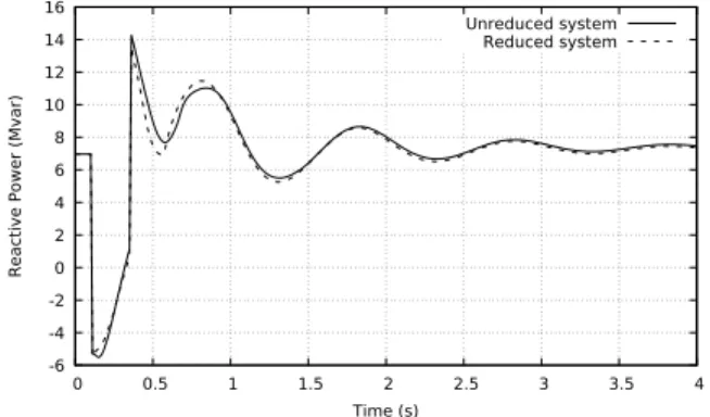
Figures 26 and 27 show the active and reactive power responses of both the unreduced and the reduced system. For the reactive power flow the accuracy is as good as it was with the training signals (see Figs. 22-24). For the active power

(10)

0 5 10 15 20 25 0 0.5 1 1.5 2 Active power (MW) Time (s) Unreduced system reduced system

Fig. 19. Training signal No. 3: Comparison of active power responses of the original and the equivalent models

0 5 10 15 20 25 30 0 0.5 1 1.5 2 Active power (MW) Time (s) Unreduced system reduced system

flow, there is still room for improvement. Indeed, while the largest excursions, immediately after the fault occurrence and immediately after its clearing, are correctly reproduced, the subsequent oscillations are too damped. The exponent α of the static load component has been found to have a significant impact: increasing α results in a better (i.e. lower) damping but also less accurate variations immediately after fault occurrence and clearing.

This also suggests that training signals involving oscillations should be considered in the future.

-6 -4 -2 0 2 4 6 8 10 12 0 0.5 1 1.5 2

Reactive Power (Mvar)

Time (s)

Unreduced system Reduced system

Fig. 22. Training signal No. 3: Comparison of reactive power responses of the original and the equivalent models

-10 -5 0 5 10 15 20 25 0 0.5 1 1.5 2

Time (s)

-10 -5 0 5 10 15 20 25 30 0 0.5 1 1.5 2

Time (s)

E. Computational efficiency

As expected, the ADN equivalent yields a high computa-tional efficiency. For instance, simulating the case of Fig. 26 takes around 0.3 s with the equivalent, and 17.1 s with the unreduced system (results on a laptop with an Intel(R) i7-6820 HQ quad-core processor @2.70 GHz, and 16 GB of RAM). Parallel processing with four threads [12] was activated when simulating the unreduced system.

The main drawback of using evolutionary algorithms is the significant computing time needed to perform the least-square

(11)

0.4 0.5 0.6 0.7 0.8 0.9 1 1.1 0 0.5 1 1.5 2 2.5 3 3.5 4 V(pu) Time (s)

Fig. 25. Voltage signal used for validation of the equivalent

0 5 10 15 20 25 0 0.5 1 1.5 2 2.5 3 3.5 4 Active power (MW) Time (s) Unreduced system reduced system

Fig. 26. Comparison of active power responses to an oscillatory signal (not used in training) given by the original and the equivalent models

-6 -4 -2 0 2 4 6 8 10 12 14 16 0 0.5 1 1.5 2 2.5 3 3.5 4

Time (s)

Fig. 27. Comparison of reactive power responses to an oscillatory signal (not used in training) given by the original and the equivalent models

minimization. Indeed, during the algorithm, new populations are generated a very large number of times and each new generation requires computing the dynamic response of the reduced system, for which the speed is independent from the optimization algorithm and cannot be shortened. However, there is still hope to improve the rate of convergence by prop-erly tuning the parameters of the DE algorithm. Alternative optimization techniques, such as derivative-free optimization, are also contemplated.

RM V XM V

RLV XLV

M

Fig. 28. Alternative structure of equivalent

VII. SUMMARY AND PERSPECTIVES

The on-going research reported in this paper aims at de-riving dynamic equivalents of distribution networks hosting significant amounts of dispersed generation. Those reduced-order models are for use at transmission level in dynamic simulations involving large disturbances. The emphasis is on PV units, although the methodology is general, and the model suits to other inverter-based generation.

First, a generic model of PV unit has been presented. It focuses on how the unit interacts with the grid, and assumes its compliance with recent grid codes. To this purpose, discrete events are taken into account such as the switching between active and reactive priority, or the tripping in low voltage conditions.

Next, a “grey-box” equivalent has been presented in which the PV units are lumped into two equivalent units according to the grid requirement they follow: one for the small residential installations, the other for the large industrial units. Each equivalent unit is represented by the above mentioned generic model. Similarly, all individual loads are lumped into a single equivalent, combining a dynamic motor and a static exponen-tial model. The resulting two units and load are connected each through a separate impedance to account for voltage drops inside the distribution network. The equivalent involves as many as 39 parameters, adjusted to match the unreduced system response in the least-square sense.

The following extensions are among those envisaged in the near future.

• While the equivalent PV units are already differentiated

by voltage levels and grid requirements, it is relevant to similarly distinguish loads according to the voltage level at which they are connected. Then, placing the two equivalent impedances in series would lead to the structure shown in Fig. 28.

• The models can be extended to include different types of

inverter-based generators with various implementations of controls and grid requirements.

• The least-square estimation of parameters minimizes the

Euclidean distance between the reference and the adjusted evolutions. Alternative accuracy measure could be con-sidered, based for instance on the metrics detailed in [24] and [25].

(12)

• The parameters θ have been estimated for one particular operating point of the unreduced system. The model validity after changes of generations and/or loads has to be assessed. In particular, it has to be checked whether simply updating the powers of the equivalent PV units and load, without re-estimating the parameters θ does not impact accuracy.

• Generally speaking, there exists some uncertainty on the

behaviour of distributed generation and even more of loads. One way to deal with this issue is to perform Monte Carlo simulations involving random variations of the parameters of the detailed, unreduced test system. Thus, for a given disturbance and a given operating point, a set of dynamic responses would be generated. The identification would be performed with respect to one representative response from this set, and the required accuracy would be selected based on the dispersion of the responses.

• The Monte Carlo simulations could also include random

measurement noise affecting Vm. This, together with

random variations of Tm (see Fig. 1) would somehow

“de-synchronize” the events taking place in PV units.

• A wider range of training signals has to be

consid-ered, involving for instance frequency deviations, voltage phase angle jumps, etc. The main motivation is to avoid “overfitting” the response to particular signals, and make the equivalent suitable for a wider range of transients in the transmission system, although most likely at the cost of a lower accuracy. The treatment of frequency deviations, for instance, will require to increase the set of parameters. Hopefully by adding training signals new subsets of parameters have their estimate improved.

ACKNOWLEDGMENT

High Performance Computational resources are provided by the “Consortium des Equipements de Calcul Intensif” (CECI), supported by the Funds for Scientific Research-FNRS, Belgium, under Grant No. 2.5020.11.

REFERENCES

[1] P. Aristidou and T. Van Cutsem, “A Parallel Processing Approach to Dynamic Simulations of Combined Transmission and Distribution Systems,” International Journal of Electrical Power & Energy Systems, vol. 72, pp. 58–65, 2015.

[2] P. Kundur, Power system stability and control. McGraw-hill New York, 1994.

[3] G. Chaspierre, “Dynamic Modeling of PV Units in response to Voltage Disturbances,” Master Thesis, University of Li´ege, 2016. Available: https://matheo.ulg.ac.be/handle/2268.2/1429.

[4] G. Kaestle and T. K. Vrana, “Improved requirements for the connection to the Low Voltage grid,” 21st International Conference on Electricity Distribution, Frankfurt, 2011.

[5] P. Kotsampopoulos, N. Hatziargyriou, B. Bletterie, and G. Lauss, “Review, analysis and recommendations on recent guidelines for the provision of ancillary services by Distributed Generation,” Proceedings 2013 IEEE International Workshop on Intelligent Energy Systems, IWIES 2013, pp. 185–190, 2013.

[6] T. Orlowska-Kowalska, F. Blaabjerg, and J. Rodrguez, Advanced and Intelligent Control in Power Electronics and Drives. Springer, 2014.

[7] Y. Bae, T. K. Vu, and R. Y. Kim, “Implemental control strategy for grid stabilization of grid-connected PV system based on German grid code in symmetrical low-to-medium voltage network,” IEEE Trans. on Energy Conversion, vol. 28, no. 3, pp. 619–631, 2013.

[8] R. Brundlinger, “Advanced smart inverter and DER functions Require-ments in latest European Grid Codes and future trends,” Solar Canada 2015 Conference, December 7, 8 2015.

[9] B. Weise, “Angle Instability of Generating Units with Fully Rated Converters in Cases of Low Voltages,” Chinese Wind and Solar Grid Integration Conference, August 7-8, 2014. Available: http://www.cwpc.cn/cwpp/files/7414/1050/5492/5-1.Presentation WiSoGIC2014 Bernd Weise Rev2 slides hidden.pdf [Accessed May, 2017].

[10] H. Soleimani Bidgoli, M. Glavic, and T. Van Cutsem, “Receding-Horizon Control of Distributed Generation to Correct Voltage or Thermal Violations and Track Desired Schedules,” Proceedings of the 19th Power System Computation Conference, 2016.

[11] C. Taylor, “Power System Voltage Stability,” Mc Graw Hill, EPRI Power Engineering Series, 1994.

[12] P. Aristidou, D. Fabozzi, and T. Van Cutsem, “Dynamic simulation of large-scale power systems using a parallel Schur-complement-based de-composition method,” IEEE Trans. on Parallel and Distributed Systems, vol. 25, no. 10, pp. 2561–2570, 2014.

[13] U. D. Annakkage, N. K. C. Nair, Y. Liang, A. M. Gole, V. Dinavahi, B. Gustavsen, T. Noda, H. Ghasemi, A. Monti, M. Matar, R. Iravani, and J. A. Martinez, “Dynamic system equivalents: A survey of available techniques,” IEEE Transactions on Power Delivery, vol. 27, no. 1, pp. 411–420, 2012.

[14] F. O. Resende, J. Matevosyan, and J. V. Milanovic, “Application of dynamic equivalence techniques to derive aggregated models of active distribution network cells and microgrids,” Proc. 2013 IEEE PES Grenoble Conference PowerTech, conf., pp. 1–6, 2013.

[15] I. Maqbool, G. Lammert, A. Ishchenko, and M. Braun, “Power System Model Reduction with Grid-Connected Photovoltaic Systems Based on Hankel Norm Approximation,” Proceedings of the 6th Solar Integration Workshop, November 2016.

[16] “Modelling and aggregation of loads in flexible power networks,” CIGRE report, 2014.

[17] M. Azmy and I. Erlich, “Identification of dynamic equivalents for distribu-tion power networks using recurrent ANNs,” IEEE PES Power Systems Conference and Exposition, 2004, pp. 721–726.

[18] S. M. Zali and J. V. Milanovic, “Generic Model of Active Distribution Network for Large Power System Stability Studies,” IEEE Trans. on Power Systems, vol. 28, no. 3, pp. 3126–3133, 2013.

[19] J. V. Milanovic and S. Mat Zali, “Validation of equivalent dynamic model of active distribution network cell,” IEEE Trans. on Power Systems, vol. 28, no. 3, pp. 2101–2110, 2013.

[20] A. Georgieva and I. Jordanov, “A hybrid meta-heuristic for global optimisation using low-discrepancy sequences of points,” Computers and Operations Research, vol. 37, no. 3, pp. 456–469, 2010.

[21] K. Fleetwood, “An Introduction to Differential Evolution ,” Available: http://www.maths.uq.edu.au/MASCOS/Multi-Agent04/Fleetwood.pdf, [Accessed January 2017].

[22] K. Price, R. M. Storn, and J. A. Lampinen, “Differential Evolution - A Practical Approach to Global Optimization,” Springer, 2005.

[23] J. Vesterstrom and R. Thomsen, “A Comparative Study of Differential Evolution, Particle Swarm Optimization, and Evolutionary Algorithms on Numerical Benchmark Problems,” Congress on Evolutionary Com-putation, 2004 CEC2004, pp. 1980—-1987, 2004.

[24] H. Sarin, M. Kokkolaras, G. Hulbert, P. Papalambros, S. Barbat, and R. J. Yang, “Comparing time histories for validation of simulation models: Error measures and metrics,” Journal of Dynamic Systems, Measurement, and Control, vol. 132, no. 6, p. 61401, 2010.

[25] D. Fabozzi and T. Van Cutsem, “Assessing the proximity of time evo-lutions through dynamic time warping,” IET Generation, Transmission & Distribution, vol. 5, no. 12, p. 1268, 2011.