Geometric Model of a Narrow Tilting CAR using Robotics formalism

HAL Id: hal-00484258

https://hal.archives-ouvertes.fr/hal-00484258

Submitted on 18 May 2010

HAL is a multi-disciplinary open access

archive for the deposit and dissemination of sci-entific research documents, whether they are pub-lished or not. The documents may come from teaching and research institutions in France or abroad, or from public or private research centers.

L’archive ouverte pluridisciplinaire HAL, est destinée au dépôt et à la diffusion de documents scientifiques de niveau recherche, publiés ou non, émanant des établissements d’enseignement et de recherche français ou étrangers, des laboratoires publics ou privés.

Geometric Model of a Narrow Tilting CAR using

Robotics formalism

Salim Maakaroun, Wisama Khalil, Maxime Gautier, Philippe Chevrel

To cite this version:

Salim Maakaroun, Wisama Khalil, Maxime Gautier, Philippe Chevrel. Geometric Model of a Narrow Tilting CAR using Robotics formalism. 15th International Conference on Methods and Models in Automation and Robotics, Aug 2010, Miedzyzdroje, Poland. paper 9011. �hal-00484258�

Geometric Model of a Narrow Tilting CAR using

Robotics formalism

Salim Maakaroun *°, Wisama Khalil*, Maxime Gautier*, Philippe Chevrel*° *Institut de Recherche en Communications et Cybernétiques de Nantes (IRCCyN)

Nantes, France

([email protected])

° Ecole des Mines de Nantes, Département d’automatique-Productique Nantes, France

([email protected]) Abstract—The use of an Electrical narrow tilting car instead

of a large gasoline car should dramatically decrease traffic congestion, pollution and parking problem. The aim of this paper is to give a unique presentation of the geometric modeling issue of a new narrow tilting car. The modeling is based on the modified Denavit Hartenberg geometric description, which is commonly used in Robotics. Also, we describe the special Kinematic of the vehicle and give a method to analyze the tilting mechanism of it. Primarily experimental results on the validation of the geometrical model of a real tilting car are given.

I. INTRODUCTION

The idea behind narrow tilting car research is to develop a narrow vehicle that seats two people in tandem [1], [2], [3]. This will reduce the size requirement of a vehicle and can be operated on reduced size lanes thereby increasing the effective capacity of highways. Moreover being an electrical car, it will provide an ecologic solution for pollution in the cities.

The aim of this paper is to present the geometric model of a specific narrow tilting car “Lumeneo Smera” [4] through the analysis of its tilting mechanism.

To model a complex system [5] in 3D motion, we use a systematic method of geometrical description, based on the modified Denavit Hartenberg parameterisation [6], [7] and. This description allows us to automatically calculate the symbolic expression of the geometric, kinematics and dynamic models by using a symbolic software package SYMORO+ [8]

This method is described in subsection 2.1 and applied on the car in subsection 2.2.

Then we analyse the tilting mechanism of the vehicle in section 3 by analysing all the loops and branches which constitute the geometrical model of the car. At the end, experimental results based on measured angles are shown to validate the geometric model of this car.

II. GEOMETRICAL DESCRIPTION OF THE TILTING CAR

A. Robotic representation of a multibody system

The car can be seen as a mobile robot which is a tree-structured multibody system composed of n bodies (links) where the chassis is the mobile base and the wheels are the terminal links. Each body Cj is connected to its

antecedent Ci (i=a (j)) with a joint that represents a

translational or rotational degree of freedom and can be elastic or rigid. A body can be virtual or real ; the virtual bodies are introduced to describe joints with multiple degrees of freedom like ball joint or intermediate fixed frames.

The frame Ri (Oi ,xi , yi , zi ) which is attached to the body Ci is defined as following:

The zi axis is along the axis of joint i, the uj axis is defined

as the common normal between zi and zj. The xi axis is

along the common normal between zi and one of the

succeeding z axis, where link i is the antecedent of link j and the origin Oi is the intersection of zi and xi.

The homogeneous transformation of the frame Ri with

respect to is expressed as a function of the following

six parameters (Fig. 1):

j i_T i

R

• γj: angle between xi and uj about zi

• bj: distance between xi and uj along zi

• αj: angle between zi and zj about uj

•dj: distance between and zzi j along uj

• θj: angle between uj and xj about zj

•rj: distance between uj and xj along zj

In (Fig.1), since xi is taken along uk, the parameters γk and bk are equal to zero.

The generalized coordinate of joint j is denoted by qj,

We define the parameter σj = 1 if joint j is translational and

σj = 0 if joint j is rotational. If there is no degree of

freedom between two frames that are fixed with respect to each other, we take σj =2.

Figure 1. Geometric parameters

B. Application for the car

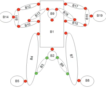
The model of the car is composed of 19 real bodies connected by 24 joints:

-B₁is the chassis

- and are two mechanical parts called “lyre” which have a rotational movement around the longitudinal axis of the chassis. is actuated by an electrical motor which controls the roll of the vehicle.

2

B B9 2

B

-B₅ and B₈are the rear wheels

- , and , are respectively the rear and left dampers of the vehicle. They are considered as rigid springs to simplify the system

3

B B6 B13 B18

- and are the rear arms that connect the chassis to the rear wheels

4

B B7

-B₁₄ and B₁₉are the front wheels

- and the chassis constitute a parallelogram which carries the hub of the left front wheel

12 11 10,B ,B

B

- and the chassis constitute a parallelogram

which carries the hub of the right front wheel

17 16 15,B ,B

B

As shown in (Fig. 2), the model is symmetric with respect to the longitudinal plan of the vehicle.

In order to study the tilting mechanism of this vehicle, we have to analyse the movement of all the loops and branches which constitute the car.

The loops are defined as follows: - LP1 is composed ofB₁,B₂,B₃and

B

₄, -LP2 is composed ofB₁,B₂,B₆andB₇,

-LP3 is composed ofB₁,B₄,B₅,B₇,B₈and the ground, -LP4 is the left parallelogram, it is composed of

and , 11 10 1,B ,B B 12 B - LP5 is composed of B₁,B₉,B₁₀andB₁₃,

-LP6 is the right parallelogram which is composed by

and , 16 15 1,B ,B B B17 - LP7 is composed ofB₁,B₉,B₁₅andB₁₈. k z i x i x j z i z j u j C i C k C j α k α

Figure 2. Description of the car III. THE TILTING MECHANISM ANALYSIS

The principle of the tilting mechanism consists of a motor turning the back lyre and tilting the chassis which leads the front lyre.

We start our study by analyzing the loop LP1 and calculating the rotation angle of the left arm according to the motorized angle of the back lyre. Then we do the same analysis on the loop LP2 to calculate the rotation angle of the right arm. After that, we study the loop LP3 which connects the rear wheels of the vehicle to the chassis and the ground, where we calculate the tilt wheel angle according to the rotation angles of the left and right arms.

At this stage, we obtain the tilt angle of the wheels which is the tilt of the vehicle since the vertical plan constituted by the four wheels is always parallel to the vertical median plan of the chassis. At last, we analyze the four front loops LP4, LP5, LP6 and LP7 and we calculate all the rotation angles of all the joints that constitute these loops.

A. Study of Loop Lp1

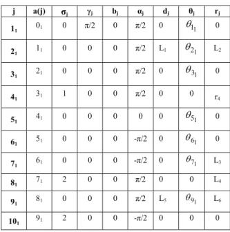
This loop is formed by the back motorized lyre, the left rear damper, the left arm and the chassis. The top of the lyre is connected to the top of the damper by a spherical joint. Also the bottom of the damper is connected to the arm through a fixed fixture by a spherical joint. Finally the other end of the arm is linked to the chassis through a rotation around the axis of the left drive electrical engine. Thus we can conclude that this chain is a closed loop starting from the axis of the lyre up the axis of the drive engine, which is fixed to the chassis.

Let R01 be a fixed reference frame attached to the chassis;

the model of this loop can be composed of 10 bodies Cj

such that (Fig. 6): j γ j d j b j θ k i u x =

- is the base attached to the chassis and is a virtual body used to define a second frame attached to the chassis,

1 0

C C₁₀₁

- is the motorized lyre

1

1

C

- and are virtual bodies used to

define the spherical joints.

1 1 1 1 3 5 6 2 ,C ,C ,C C 1 7 C - is the damper 1 4 C

- is the arm and is a virtual body attached to the arm

1

9

C C₈₁

We model this loop as a serial chain by imposing a constraint on the terminal frame depending on the position and orientation.

Figure 3. Description of loop LP1

TABLE I. GEOMETRIC PARAMETERS OF LOOP LP1

j a(j) σj γj bj αj dj θj rj 11 01 0 π/2 0 π/2 0 θ11 0 21 11 0 0 0 π/2 L1 θ21 L2 31 21 0 0 0 π/2 0 θ31 0 41 31 1 0 0 π/2 0 0 r4 51 41 0 0 0 0 0 θ51 0 61 51 0 0 0 -π/2 0 θ61 0 71 61 0 0 0 -π/2 0 θ71 L3 81 71 2 0 0 π/2 0 0 L4 91 81 0 0 0 π/2 L5 θ91 L6 101 91 2 0 0 -π/2 0 0 0

The imposed constraint on the terminal frame consists of fixing it to the chassis as the frame R0. Thus these two

frames move at the same time and in the same way when the vehicle tilts. The only difference is at the level of the position.

Therefore the resolution of the constraint equations corresponds to the resolution of the inverse geometric

model IGM that gives all the robot configurations corresponding to a given location of the end effector. The 4x4 homogenous transformation matrix between

and is: 1 1 1 0_T 1 0 R 1 10 R (1) ⎥ ⎥ ⎥ ⎥ ⎦ ⎤ ⎢ ⎢ ⎢ ⎢ ⎣ ⎡ = 1 0 0 0 1 0 0 0 1 0 0 0 1 1 1 10 0 z y x P P P T

Where P ,_x P_yand Pzare the position coordinate of the

frame R101 with respect to the frame R01.

This serial chain has one motorized joint and six passives joints and . Since there are three rotation joints of convergent axes, the maximum number of solutions must be 8 [9].

We apply the numerical algorithm in appendix A on this loop and we obtain 8 possible configurations. To visualize which of these solutions corresponds to the real configuration of the chain, we use Corke Robotics Toolbox [10] on Matlab to draw the solutions (Fig. 4).

Figure 4. Simulation of a solution of LP1

B. Study of loop LP2

The architecture of this loop is the same as loop LP1 but in the opposite direction (fig.5). That means if the left arm goes up, then the right arms goes down due to the symmetric architecture of rear train.

We analyse this loop in the same way as loop LP1 to obtain at the end the rotation angle of the right arm.

Figure 5. Description of loop LP2

1 1 1, 7 , ,θ θ θ θ θ_{21 31 4 6}, θ1₁ θ11

TABLE II. GEOMETRIC PARAMETERS OF LOOP LP2 j a(j) σj γj bj αj dj θj rj 11 01 0 π/2 0 π/2 0 θ11 0 22 11 0 0 0 -π/2 L1 θ22 L2 32 22 0 0 0 -π/2 0 θ32 0 42 32 1 0 0 π/2 0 0 r4 52 42 0 0 0 0 0 θ52 0 62 52 0 0 0 - π/2 0 θ62 0 72 62 0 0 0 π/2 0 θ72 L3 82 72 2 0 0 π/2 0 0 L4 92 82 0 0 0 -π/2 L5 θ92 L6 102 92 2 0 0 π/2 0 0 0 C. Study of loop LP3

The left and right wheels, the left and right arms and the chassis form this loop. The entire joints between the bodies of this structure are rotational.

Let R03 be a fixed reference frame attached to the ground;

the model of this loop can be composed of 10 bodies such that (Fig. 6):

j C

- is the base attached to the ground and are two virtual bodies used to define two frames attached to the ground

3 0

C C₉₃,C₁₀₃

- is the right wheel and is a virtual body attached to it,

3 1

C C₂₃

- ₃is the left arm and is a virtual body fixed to the arm,

4

C C3₃

- is the right arm and is a virtual body attached to it,

3 5

C C₆₃

- is the left wheel and is a virtual body attached to it.

3 8

C C7₃

The joints 1 and 8 represent the tilt of the wheels and consequently the tilt of the vehicle.

Figure 6. Description of loop LP3

TABLE III. GEOMETRIC PARAMETERS OF LOOP LP3

j a(j) σj γj bj αj dj θj rj 13 03 0 π/2 0 π/2 0 θ13 0 23 13 2 0 0 π/2 0 π/2 R 33 23 0 0 0 π/2 0 θ33 L7 43 33 0 0 0 0 L8 0 0 53 43 0 0 0 0 0 θ53 L9 63 53 0 0 0 0 L8 θ63 L7 73 63 2 0 0 π/2 0 θ73 -R 83 73 0 0 0 π/2 0 0 0 93 83 2 0 0 π/2 0 θ93 0 103 93 2 0 0 π/2 0 0 0

We apply the algorithm in appendix A to this serial chain with the constraint equation between the frame and . As tires stay always in touch with the ground, we can say that Pz=0 and the error will be on and

. 1 0 R

)

1 10 R 4 , 3 ( c

3

(:,

c

dX

) dX

For a given angle of the rotation of the back lyre, we resolve respectively loop1, loop2 and loop3 by making the necessary changes for the offsets of the joints between the different loops; thus we calculate the tilt of the vehicle. The shape of the loop3 can be shown in figure (7) after applying an angle of rotation to the back lyre by using Corke robotics Toolbox (Fig. 7).

Figure 7. Simulation of loop LP3

Since the motion of all the front loops is planar, we will analyze analytically the geometric model of these loops. The principle of the analysis of closed loops consists on treating the equivalent tree structure that is obtained by cutting each closed loop at one of its joints and by adding two frames at each cut joint. The total number of frames is equal to n + 2B and the geometric parameters of the last B frames are constants. Thus, the position and orientation of all the links can be determined as a function of the active joint variables.

Loop Lp4 is at first analyzed in order to determine the relations between the various variables of the joints of this chain for a given tilt angle of the chassis.

Then we treat loop LP5, by considering shock absorbers also blocked as (section 3.1 and 3.2) and from the same given tilt angle, we calculate the rotation angle of the front lyre.

At this stage, we follow the reverse path across the lyre, by analysing loop7 corresponding to the calculated angle of the lyre in loop5.

At the end, the study of Loop 6 is similar to Loop 4.

D. Study of loop LP4

Let R04 be a fixed reference frame attached to the chassis;

the model of this loop can be composed of 5 bodies Cj

such that (Fig .8):

-C₀₄is the base attached to the chassis, -C₁₄is the bottom arm of the left parallelogram -C₂₄is the upper arm of the parallelogram

- ₄is always parallel to the chassis and caries the hub of the left wheel,

3 C

- ₄and ₄are two equal virtual bodies attached to but with different antecedent

4

C C5 C34

Figure 8. Description of loop LP4

TABLE IV. GEOMETRIC PARAMETERS OF LOOP LP4

j a(j) σj γj bj αj dj θj rj 14 04 0 0 0 0 0 θ14 0 24 04 0 0 0 0 L10 θ24 0 34 14 0 γ34 0 0 L11 θ34 0 44 24 0 0 0 0 L11 θ44 0 54 24 2 0 0 0 L10 0 0 Let 4 1

θ be the actuated joint of this loop and its value equal to the tilt of the vehicle. The symbolic resolution of the geometric constraint equations of Loop 4 is calculated by using a symbolic software SYMORO+ [7]:

0

4 4 4 4 4 1 3 2 4 3

+

θ

+

θ

−

θ

−

θ

=

γ

(2) 4 4 4 2 3 1

θ

γ

θ

+

=

(3)

0

4 4 4 1 3 3

+

θ

+

θ

=

γ

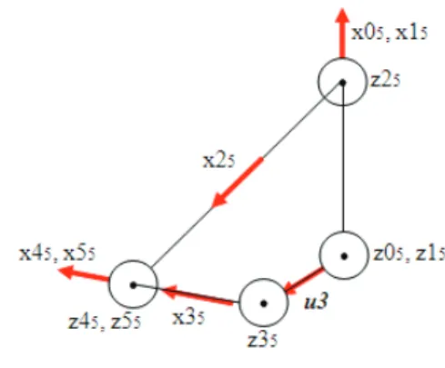
(4) E. Study of loop LP5

Let R05 be a fixed reference frame attached to the chassis;

the model of this loop can be composed of 5 bodies Cj

such that (Fig. 9):

-C₀₅is the base attached to the chassis -C₁₅is the front lyre

-C₂₅is the left blocked damper

-C₃₅is the bottom arm of the left parallelogram,

- and ₅are two equal virtual bodies attached to but with different antecedent

5 4 C 5 3 C 5 C

Figure 9. Description of loop LP5

The geometric parameters of loop LP5 are the same as loop LP4 with the following modifications:

a(25)=15; a(35)=05; d25 = L12; d35 = L15; d45 = L13; d55 = L13

Let be the actuated joint of this loop. The geometric constraint equations of Loop LP5 are given by using SYMORO+: o =θ θ γ35 −θ15 −θ25 +θ35 −θ4₅=0 (5) ₎ 2 cos 2 cos( 13 12 3 15 14 2 14 2 15 2 13 2 12 25 L L 5 L L L L L L a θ θ =± − − + + + (6) 0 ) cos( cos cos 3₅ 13 4₅ 12 2₅ 4₅ 14 15+L θ −L θ −L θ +θ = L (7)

sin sin sin( ) 0

5 5 5 5 13 4 12 2 4 3 14 + + + = −L θ L θ L θ θ (8)

Since the architecture of the loop, we select the positive value of equation (6). θ45is calculated from (7) and (8) :

₄ tan(sin( ₄ ),cos( ₄₅)) 5 5

θ

θ

θ

=a

(9)

Where 5 5 5 5 5 5 2 12 13 2 12 2 13 3 14 15 2 12 3 14 2 12 13 4 cos 2 ) cos ( sin ) sin )( cos ( sin θ θ θ θ θ θ L L L L L L L L L L + + + − + = 5 5 5 2 13 12 2 12 2 13 3 14 2 12 3 14 15 5 2 12 13 4 cos 2 sin sin ) cos )( cos ( cos θ θ θ θ θ θ L L L L L L L L L L + + + + + = ff + 4 5 1 3

At the end, θ15 is calculated by (5). F. Study of loop LP6 and LP7

The analysis of LP6 and LP7 is respectively the same as LP4 and LP5 with these modifications:

-we study LP7 before LP6,

-the actuated joint of LP7 is θ17and is equal to θ15

calculated in (5),

-

the actuated joint of LP6 is θ16 and is equal to θ37 +off

calculated in LP7.

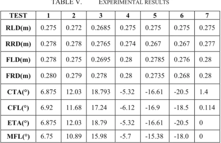
IV. EXPERIMENTAL RESULTS

Primarily experimental results are given. For the data acquisition, a real tilting car is equipped with many sensors which allow the validation of the geometrical model. Those sensors are: a position sensor, 3 gyroscopes and 3 accelerometers. They allow us to specify the rotation angle of the front lyre and the tilt of the vehicle.

A. Results

TABLE V. EXPERIMENTAL RESULTS

TEST 1 2 3 4 5 6 7 RLD(m) 0.275 0.272 0.2685 0.275 0.275 0.275 0.275 RRD(m) 0.278 0.278 0.2765 0.274 0.267 0.267 0.277 FLD(m) 0.278 0.275 0.2695 0.28 0.2785 0.276 0.28 FRD(m) 0.280 0.279 0.278 0.28 0.2735 0.268 0.28 CTA(°) 6.875 12.03 18.793 -5.32 -16.61 -20.5 1.4 CFL(°) 6.92 11.68 17.24 -6.12 -16.9 -18.5 0.114 ETA(°) 6.875 12.03 18.79 -5.32 -16.61 -20.5 0 MFL(°) 6.75 10.89 15.98 -5.7 -15.38 -18.0 0 Where:

RLD, RRD, FLD and FRD are respectively the rear left and right dampers and the front left and right dampers; CTA and CFL are respectively the calculated tilt angle and the calculated front lyre angle;

ETA and MFL are respectively the estimated tilt angle and the measured front lyre angle. The ETA is obtained from the accelerometers with the aim of cancelling the effect of the centrifugal force.

By comparing the measured or estimated angles and the calculated angles, we conclude that margin of error is between [0°, 2°]. Therefore the geometric model is validated.

V. CONCLUSIONS

Despite the validation of the geometric model, it is important to notice that all tests have been realized with blocked dampers and this case does not reflect the reality. Therefore we have to consider later the elasticity of the

dampers in order to calculate the dynamic model of the vehicle, to identify the dynamic parameters and finally to simulate the behaviour of the car. Future work will concern the identification of the dynamic parameters and the control of the lyre angle to ensure the stability of the vehicle.

REFERENCES

[1] Gohl J., Rajamani R. and al , Development of a Novel Tilt-Controlled Narrow Commuter Vehicle, (internal report) May 2006. [2] So SG., Karnopp D Active dual mode tilt control for narrow

ground vehicle, Vehicle System Dynamics journal, vol 27, pp19-36 1997.

[3] Hibbard R., Karnopp D, the dynamics of small, relatively tall and narrow tilting ground vehicle, ASME Dynamics Systems and Control, 52, pp. 397-417 1992.

[4] Lumeneo, www.lumeneo.fr

[5] Rajamani R., vehicle dynamics and control, Springer 2005 [6] Khalil W., Kleinfinger J.F., A new geometric notation for open and

closed loop robots, Proc. IEEE on robotics and automation, pp. 1174- 1180, San Francisco, CA, USA 1986.

[7] Khalil W., Creusot D, SYMORO+: a system for the symbolic modelling of robots, Robotica, Vol. 15, 1997, p. 153-161 1997. [8] Pieper D. (1968), The kinematics of manipulators under computer

control , PhD Thesis, Stanford University, UK 1968.

[9] Corke P.., A Robotics Toolbox for MATLAB, IEEE on robotics and automation, N01, pp. 24-32-, vol 3 1996.

[10] Khalil W. and Dombre E. , Modelling, identification and control of robots, Hermès Penton, London & Paris 2002 .

APPENDIX A:NUMERICAL CALCULATION OF THE INVERSE GEOMETRIC MODEL

When it is not possible to find an explicit form to the inverse geometric model, we can use the Kinematic model to calculate recursively numerical solution qd

corresponding to a desired situation . The algorithm is defined as:

n d T

0

-Define an initial random configuration_qc, -Calculate the direct geometrical model corresponding to this configuration,

n c T

0

-Calculate the error between

and , where dX and

[

_TT r T p c dX dX dX = c n d n p =P −P

]

0Tdn n c T 0 _{dX uα} r = - Define a threshold

S

to dX_c: If dXc > then, S

Else Stop the calculation and _qd will be equal to_qc. -Calculate numerically the direct Jacobian matrix and her pseudo-inverse ,

) ( 0 c nq J + J

-Calculate dq=J+_{dX then update the current}

configuration: qc_{= q}c_{+dq and return to the second step.}

We notice that if the algorithm does not converge after a predefined number of iterations, or if we need to obtain another different solution, it is necessary to begin again the calculation with a new initial value.

S dX_c c= dXc dX