HAL Id: hal-02947222
https://hal.archives-ouvertes.fr/hal-02947222
Submitted on 23 Sep 2020
HAL is a multi-disciplinary open access
archive for the deposit and dissemination of
sci-entific research documents, whether they are
pub-lished or not. The documents may come from
L’archive ouverte pluridisciplinaire HAL, est
destinée au dépôt et à la diffusion de documents
scientifiques de niveau recherche, publiés ou non,
émanant des établissements d’enseignement et de
Synthesis of 3-RPS Parallel Manipulators based on
Prescribed Operation Modes
Latifah Nurahmi, Stéphane Caro, Philippe Wenger
To cite this version:
Latifah Nurahmi, Stéphane Caro, Philippe Wenger. Synthesis of 3-RPS Parallel Manipulators based
on Prescribed Operation Modes. The 4th IFTOMM International Symposium on Robotics and
Mecha-tronics, Jun 2015, Poitiers, France. �hal-02947222�
on Prescribed Operation Modes
Latifah Nurahmi, St´ephane Caro, Philippe Wenger
Institut de Recherche en Communications et Cybern´etique de Nantes,
Emails:{latifah.nurahmi,stephane.caro,philippe.wenger}@irccyn.ec-nantes.fr
Abstract. The subject of this paper is about the synthesis of the design parameters by
consider-ing the prescribed operation modes at the design stage for a parallel manipulator with three RPS legs. The synthesis is based on the Euler parametrization and the results of primary decomposi-tion. The design parameters and the coordinates of one RPS leg are initially defined to formulate the constraint equation associated with this leg. Seven classes of the RPS leg are identified and the geometric properties of each class are highlighted. By selecting three different or identical classes of the RPS leg, a new 3-RPS parallel manipulator is proposed without specific values of the design parameters. The primary decomposition is computed over a set of three constraint equations. One or more Euler parameters in the results of primary decomposition is constrained to be equal to null, which leads to particular type of operation mode. The methodology also provides new archi-tectures of the 3-RPS parallel manipulators based on a classification of the RPS leg, that satisfy the prescribed operation mode.
Key words: Synthesis, design parameters, primary decomposition, operation mode, RPS legs.
1 Introduction
The well-known 3-RPS (R, P, S, represent revolute, prismatic, and spherical, re-spectively) parallel manipulator with different shapes of moving platform and base was extensively studied by many researchers. In 1983 [4], Hunt introduced the 3-RPS manipulator which has an equilateral triangle base and an equilateral triangle platform. Schadlbauer et al. in [7] revealed that this manipulator has two distinct operation modes and in [6] the authors characterized the type of motion in both op-eration modes by using the axodes. Huang et al. in 1995 [2] proposed the 3-RPS cube manipulator which is composed of a cube-shaped base and an equilateral tri-angle platform. By using the Study kinematic mapping, Nurahmi et al. in [5] found that this manipulator has only one operation mode in which the 3-dof general mo-tion and the Vertical Darboux Momo-tion occur inside the same operamo-tion mode.
Accordingly, a general approach to synthesize the design parameters by con-sidering the prescribed operation modes for a parallel manipulator with three RPS legs, is discussed in more details in this paper. The approach is based on the Euler parametrization [1], and the primary decomposition is used to reveal the existence of the number and the type of operation modes [8]. The first essential step is to
2 Latifah Nurahmi, St´ephane Caro, Philippe Wenger characterize the coordinates and to define the design parameters of one RPS leg. Then, the constraint equation of this RPS leg is formulated by means of the Euler parametrization. A classification of seven classes of the RPS legs are found, which gives a general information about the position and the orientation of the RPS legs. By selecting three different or identical classes of the RPS legs, a new 3-RPS manip-ulator is generated without specific value of the design parameters. The constraint equations of the corresponding new manipulator are derived and the primary de-composition is computed. By restricting one or more Euler parameters to be equal to null, the design parameters can be synthesized.
2 Coordinates and design parameters of RPS leg
x0 y0 z0 x1 y1 z1 O P αi βi εi ζi ai bi Σ0 Σ1
A
iB
is
iFig. 1: Coordinates and Design Parameters of RPS Leg. x0 y0 z0 O γi Γi Σ0
s
iFig. 2: The axis of revo-lute joint.
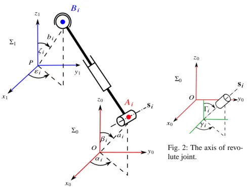
The RPS leg shown in Fig. 1, is composed of a revolute joint, a prismatic joint, and a spherical joint mounted in series. The revolute joint is attached to the base and denoted by point Ai1. This point is located in the three-dimensional space which
is specified by the azimuth angle αi, the polar angle βi, and the radial distance ai
from the origin O of the fixed frame Σ0.
azimuth angle εi, the polar angle ζi, and the radial distance bi from the origin P of
the moving frame Σ1. The axis of the revolute joint is along the vector si, which is
specified by the azimuth angle γiand the polar angle Γi(Fig. 2). The coordinates of
points Ai, Bi and unit vector si are:
r0A i= h 1, cαicβiai,sαicβiai,sβiai iT , r1B i= h 1, cεicζibi,sεicζibi,sζibi iT si= h 0, cγicΓi,sγicΓi,sΓi iT . (1) where cαi= cos(αi), sαi= sin(αi), cβi= cos( βi), sβi= sin( βi), cεi= cos(εi), sεi=
sin(εi), cζi = cos(ζi), sζi = sin(ζi), cγi = cos(γ), sγi = sin(γ), cΓi = cos(Γ), and
sΓi = sin(Γ). As a consequence, there are eight design parameters for one RPS leg,
namely ai, bi, αi, βi, εi, ζi, γi, and Γi. Since the manipulator that will be created
should have three RPS legs, hence there are 24 design parameters in the 3-RPS manipulator.
3 Constraint Equations
In this section, the constraint equation is expressed for one RPS leg shown in Fig. 1. To obtain the coordinates of point Biexpressed in Σ0, the transformation matrix M2
by means of the Euler parametrization [1] is used.
The parameters x0,x1,x2,x3, which appear in matrix M, are called Euler
param-eters of the rotation. They are useful in the representation of a spatial Euclidean displacement and they should satisfy the equation [3]: x20+ x21+ x22+ x23− 1 = 0. This condition will be used in the following computations to simplify the algebraic ex-pressions. The coordinate of point Biexpressed in Σ0is obtained by: r0Bi = M r
1 Bi.
As the coordinates of all points are given in terms of the Euler parameters and the design parameters, the constraint equation can be obtained by examining the design of the RPS leg. The leg connecting points Ai and Bi is orthogonal to the axis si of
the revolute joint. Accordingly, the scalar product of vector (r0Bi− r0A
i) and vector si vanishes, namely: (r0Bi− r 0 Ai) T s i= 0.
After computing the corresponding scalar products and removing the common denominators the following constraint equation of one RPS leg comes out:
hi : cγicΓiX + cΓisγiY + (x 2 0− x 2 1− x 2 2+ x 2 3)sζisΓibi− sβisΓiai+ (2x1x2− 2x0x3)bi cΓicγisεicζi+ (2x0x3+ 2x1x2)bisγicΓicζicεi+ (x 2 0+ x 2 1− x 2 2− x 2 3)cεicζicγicΓibi − cαicβicγicΓiai+ (x 2 0− x 2 1+ x 2 2− x 2 3)cζisεicΓisγibi− cβicΓisαisγiai+ (2x0x1+ 2x2x3)bisΓisεicζi+ (2x0x2+ 2x1x3)bicΓicγisζi+ (2x2x3− 2x0x1)bisγicΓisζi+ (2x1x3− 2x0x2)bisΓicζicεi+ sΓiZ = 0 (2)
2For detail expression of the transformation matrix, the reader may refer to
4 Latifah Nurahmi, St´ephane Caro, Philippe Wenger
4 Classifications of the RPS legs
In this section, the constraint equation associated with the design parameters are solved to synthesize seven classes of the RPS legs. The constraint equation hi in
Eq. (2) should vanish in any condition, likewise in the identity condition. In the identity condition Σ0and Σ1are coincident, and we have the identity transformation
I in which the parameters become x0= 1, x1= 0, x2= 0, x3= 0, X = 0, Y = 0, Z = 0. By substituting these values into Eq. (2), this yields:
hI: (cεicζicγicΓi+ cζicΓisεisγi+ sζisΓi)bi− (cαicβicγicΓi+ cβicΓisαisγi
+ sβisΓi)ai= 0
(3)
Eq. (3) can be written as hI: f − g = 0. To find the relations between the design parameters for which hIvanishes, we compute one particular condition where f , g vanish simultaneously. Note that it also amounts to the condition to be fulfilled for which hIvanishes no matter the values of ai and bi. One has to discuss the ideal
I = h f , gi and compute the Groebner basis. The relations containing complex terms are discarded and 23 relations remain, and substituted into Eq. (1). Based on their geometric properties, seven classes are identified and each class contains one or more sub-classes3. The sub-classes give the location of the RPS legs in the three-dimensional space, in which r0A
i gives the location of the revolute joint with respect
to Σ0, r1Bi gives the location of the spherical joint with respect to Σ1, and si gives
the unit vector of the axis of the revolute joint.
By selecting three different or identical classes, a new manipulator with three RPS legs can be created. The user may assign some arbitrary values into the design parameters and assemble the legs accordingly. However, it is interesting to generate various designs of the 3-RPS manipulator that fulfil the prescribed operation modes as presented in the following.
5 Synthesis of Design Parameters
In the following, an example of 3-RPS manipulator with three identical classes of the RPS leg will be presented. Then, the design parameters associated with the new manipulator are synthesized by imposing the prescribed operation modes.
5.1 Sub-class F.2
In this section, the 3-RPS manipulator is generated by selecting three identical sub-classes, namely sub-class F.2. The RPS leg in this class consists of revolute joint and spherical joint that are located in any position with respect to Σ0and Σ1, respectively.
The axis of the revolute joint is parallel to the xy-plane.
Due to the heavy computations, points Ai and Bi are assumed to lie in the
β3= 0 and ζ1= ζ2= ζ3= 0. The first RPS leg of the manipulator is fixed by sub-stituting ε1= 0. To obtain the coordinates of points B1, B2, B3expressed in Σ0, the
coordinate transformation is performed by means of the Euler parametrization as: r0
Bi= M r
1
Bi (i = 1, 2, 3). The constraint equations are determined by computing the
scalar products of the vector AiBi and the unit vector si which has to vanish as:
(r0 Bi− r
0 Ai)
T s
i= 0. The constraint equations turn out: h1: Y + (2x0x3+ 2x1x2)b1= 0 h2: 4c2ε2b2x1x2− 2(x 2 1− x 2 2)cε2sε2b2+ cε2Y− sε2X + (2x0x3− 2x1x2)b2= 0 h3: 4c2ε3b3x1x2− 2(x 2 1− x 2 2)cε3sε3b3+ cε3Y− sε3X + (2x0x3− 2x1x2)b3= 0 (4)
For the algebraic computation, the half-tangent substitutions are performed to re-move the trigonometric functions in the second and the third legs: sεi= (2tei)/(1 +
te2i), cεi = (1− te
2
i)/(1 + te 2
i), i = 2, 3. Then the three constraint equations are
written as polynomial idealI = hh1,h2,h3i with variables {x0,x1,x2,x3,X,Y, Z}
over the coefficient ring C[b1,b2,b3,te2,te3]. The primary decomposition is
com-puted and it turns out thatI does not decompose, i.e. it has general expressions as I = hg1,g2,g3i, as follows4: g1: (2b2te32te33− 2b3te32te33+ 2b2te32te3− 2b2te2te33+ 2b3te23te3− 2b3te2te33... g2: Y (b1te42te33− b1te 3 2te 4 3+ b2te42te33− b3te 3 2te 4 3+ b1te42te3− b1te2te43− b3te2... g3: X (b1te42te33− b1te 3 2te 4 3+ b2te42te33− b3te 3 2te 4 3+ b1te42te3− b1te2te43+ b2te24... (5) It can be seen from Eq. (5) that g1,g2,g3 are free of Z component. This means
that for any value of the design parameters (b1,b2,b3, ε2, ε3), the manipulator can
always perform a pure translation along z direction. Variable x3can be solved
lin-early from g1and x3is parametrized by x0,x1,x2. This means that the manipulator
is capable of orientations determined by x0,x1,x2 in which variable x3is not null.
Equations g2,g3 can be solved linearly for variables Y and X , respectively. This
shows that the manipulator undergoes translational motions along x and y directions which are coupled to the orientations. In the following, the rotational components {x0,x1} from g1,g2,g3are constrained to be equal to zero, which leads to different
operation modes. By fulfilling this condition, the design parameters are synthesized and new architectures are proposed.
5.1.1 Case x0= 0
One variable is constrained to be null, namely x0= 0. Since only the equation g1
has component x0, the computation will be carried out only for g1. After substituting
x0= 0, equation g1becomes: g1: a x12+ bx1x2+ cx22= 0, where a, b, c are polynomial coefficients in terms of the design parameters (b1,b2,b3,te2,te3).
To synthesize the design parameters, all polynomial coefficients have to vanish. Hence, one has to discuss the idealJ = ha, b, ci. The Groebner basis of the ideal J
4For complete results of the primary decomposition, the reader may refer to
6 Latifah Nurahmi, St´ephane Caro, Philippe Wenger is computed and 17 solutions of the design parameters are obtained. Not all solutions are possible and hence some assumptions are developed, as follows:
1. The second and the third legs cannot be coincident with the first leg: - ε2,0 and ε3,0
2. The second leg cannot be coincident with the third leg: - ε2,ε3
3. The magnitude of bi (i = 1, 2, 3) should be positive:
- bi≥ 0, i = 1, 2, 3
4. The platform cannot be a point: - b1,b2,b3,0
5. No complex solutions: -{b1,b2,b3, ε2, ε3} ∈ R
After removing the solutions that do not fulfil the assumptions stated above, four solutions of the design parameters are obtained. The solutions are:
L1: b2= 0, b3= 0, ε3= π + ε2 L2: b2= b1 tan(ε3) , b3= 0, ε2= π 2, ε3,0 or ε3,±π L3: b2=− b1 tan(ε3) , b3= 0, ε2=− π 2, ε3,0 or ε3,±π L4: b1= b3 cos(ε2− ε3) cos(ε2) , b2= b3 cos(ε3) cos(ε2) , ε2,± π 2 or ε2,± 3π 2 (6)
The 3-RPS manipulator can be generated by selecting one of the solutions (L1,L2,L3,L4). In the following, the application of the solution L2is presented.
Solution L2
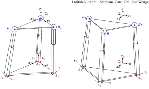
In solution L2, some values are assigned as b1= 1 and ε3=−2π/3. Other design parameters are obtained as: b2=
√
3/3, b3= 0, ε2= π/2. The new architecture of the 3-RPS manipulator is depicted in Fig. 3. The base and the moving platform have right-angle triangle shape. The unit vectors s1and s2are orthogonal (s1⊥ s2).
The values of the design parameters are substituted into the set of three constraint equations defined in Eq. (4). The primary decomposition is computed and it shows that the mechanism has two operation modes as follows: K =T2
i=1Ki, with the
results of primary decomposition: K1=hx0,3X− √ 3Y, 2x1x2+ Yi K2=hx3,3X− √ 3Y, 2x1x2+ Yi (7) First operation mode is shown by the first sub-ideal K1, in which x0= 0. All possible poses of the mechanism in this operation mode are obtained by rotating the platform from the identity condition about a transformation axis by π and translating along the same direction. Second operation mode is shown by the sub-idealK2with
5.1.2 Case x1= 0
In this section, the variable x1 in Eq. (5) is constrained to be null. After
comput-ing the Groebner basis, 11 solutions of the design parameters are obtained. Not all solutions are possible and hence by following the aforementioned assumptions in Section 5.1.1, three solutions are obtained as:
L1: b2=− b1 tan(ε3) , b3= 0, ε2= π 2, ε3,0 or ε3,±π L2: b2= b1 tan(ε3) , b3= 0, ε2=− π 2, ε3,0 or ε3,±π L3: b1=−b3 cos(ε2− ε3) cos(ε2) , b2= b3 cos(ε3) cos(ε2) , ε2,± π 2 or ε2,± 3π 2 (8)
By choosing one of the solutions (L1,L2,L3), a new 3-RPS manipulator can be
built. The application of the solution L3 is presented in the following.
Solution L3
Solution L3 is selected to generate the 3-RPS manipulator whose operation
modes contain x1= 0. The design parameters b3= 1, ε2= π/4, and ε3=−π/4 are assigned, hence b1=
√
2 and b2= 1 are determined. The 3-RPS manipulator with these design parameters is depicted in Fig. 4, in which the base and the moving plat-form have right-angle triangle shape. The axes of the second and the third revolute joints are orthogonal and meet at point A1.
The values of the design parameters are substituted into the set of three constraint equations defined in Eq. (4). The primary decomposition is computed and it shows that the mechanism has two operation modes as follows: K =T2
i=1Ki, with the
results of primary decomposition: K1=hx1,4x0x3+ √ 2Y, 2x22−√2Xi K2=hx2,4x0x3+ √ 2Y, 2x21+√2Xi (9)
The sub-idealK1 shows the first operation mode of this manipulator, in which
x1= 0. In this operation mode, the moving platform is transformed from the identity condition about an axis parallel to the yz-plane. The second operation mode of this manipulator is shown by sub-idealK2with x2= 0. The transformation axis of this operation mode is parallel to the xz-plane.
6 Conclusions
In this paper, the synthesis of the design parameters corresponding to the prescribed operation modes for a parallel manipulator with three RPS legs was addressed. The Euler parametrization and the results of primary decomposition were used to define the synthesis procedure by considering the type of operation modes at the design stage. The design parameters and the coordinates of one RPS leg were initially defined. Then, the constraint equation corresponding to the RPS leg was derived. Seven classes of the RPS legs were developed, in which each class contains several sub-classes that corresponds to the specific position and orientation of the RPS legs.
8 Latifah Nurahmi, St´ephane Caro, Philippe Wenger x0 y 0 z0 x1 y 1 z1 Σ0 Σ1 s1 s2 s3 A1 A2 A3 B1 B2 B3
Fig. 3: Design with solution L2.
x0 y0 z0 x1 y1 z1 Σ0 Σ1 s1 s2 s3 A1 A2 A3 B1 B2 B3
Fig. 4: Design with solution L3.
As a result, it is possible to generate new architectures of the 3-RPS manipulator by selecting three different or identical classes of the RPS legs. Some constraints were applied to the Euler parameters in the results of primary decomposition that leads to particular types of operation modes, and then the design parameters were synthesized. Several architectures of the 3-RPS manipulators corresponding to the prescribed operation modes were presented. The applications of the proposed ap-proach for parallel manipulators with different type of legs, will be the subject of future research.
References
1. Bottema, O., Roth, B.: Theoretical Kinematics. Dover Publishing New York, pp. 304-322 (1990)
2. Huang, Z., Fang, Y.: Motion Characteristics and Rotational Axis Analysis of Three DOF Paral-lel Robot Mechanisms. In Proceedings of the 1995 IEEE International Conference on Systems, Man and Cybernetics, Vol. 1, pp. 67-71 (1995)
3. Husty, M. L., Pfurner, M., Schr¨ocker, H-P., Brunnthaler, K.: Algebraic Methods in Mechanism Analysis and Synthesis. Robotica, 25(6) pp. 661-675 (2007).
4. K.H. Hunt.: Structural Kinematics of in-parallel-actuated Robot-arms. Journal of Mechanisms, Transmissions, and Automation in Design, 105 pp. 705-712 (1983).
5. Nurahmi, L., Schadlbauer, J., Caro, Stephane., Husty, M., Wenger, P.: Kinematic Analysis of the 3-RPS Cube Parallel Manipulator. Journal of Mechanisms and Robotics, 7(1) pp. 011008-1011008-10 (2015).
6. Schadlbauer, J., Nurahmi, L., Husty, M., Wenger, P. and Caro, S.: Operation Modes in Lower-Mobility Parallel Manipulators, Second Conference on Interdisciplinary Applications of Kine-matics, Lima, Peru, September 9–11, (2013).
7. Schadlbauer, J., Walter, D.R., Husty, M.: The 3-RPS Parallel Manipulator from an Algebraic Viewpoint. Mechanism and Machine Theory, 75 pp.161-176 (2014).