Dynamic Parameter Identification of a 6 DOF Industrial Robot using Power Model

(1)

HAL Id: hal-00770758

https://hal.archives-ouvertes.fr/hal-00770758

Submitted on 25 Jun 2019

HAL is a multi-disciplinary open access

archive for the deposit and dissemination of

sci-entific research documents, whether they are

pub-lished or not. The documents may come from

teaching and research institutions in France or

abroad, or from public or private research centers.

L’archive ouverte pluridisciplinaire HAL, est

destinée au dépôt et à la diffusion de documents

scientifiques de niveau recherche, publiés ou non,

émanant des établissements d’enseignement et de

recherche français ou étrangers, des laboratoires

publics ou privés.

Robot using Power Model

Maxime Gautier, Sébastien Briot

To cite this version:

Maxime Gautier, Sébastien Briot. Dynamic Parameter Identification of a 6 DOF Industrial Robot

using Power Model. the 2013 IEEE International Conference on Robotics and Automation (ICRA

2013), May 2013, Karlsruhe, Germany. �hal-00770758�

(2)



Abstract—Off-line dynamic identification requires the use of

a model linear in relation to the robot dynamic parameters and the use of linear least squares technique to calculate the parameters. Most of time, the used model is the Inverse Dynamic Identification Model (IDIM). However, the computation of its symbolic expressions is extremely tedious. In order to simplify the procedure, the use of the Power Identification Model (PIM), which is dramatically simpler to obtain and that contains exactly the same dynamic parameters as the IDIM, was previously proposed. However, even if the identification of the PIM parameters for a 2 degrees-of-freedom (DOF) planar serial robot was successful, its fails to work for 6 DOF industrial robots. This paper discloses the reasons of this failure and presents a methodology for the identification of the robot dynamic parameters using the PIM. The method is experimentally validated on an industrial 6 DOF Stäubli TX-40 robot.

I. INTRODUCTION

EVERAL schemes have been proposed in the literature to

identify the dynamic parameters of robots [1]–[7]. Most of the dynamic identification methods have the following common features:

- the use of a model linear in relation to the dynamic parameters,

- the construction of an over-determined linear system of equations obtained by sampling the model while the robot is tracking some trajectories in closed-loop control,

- the estimation of the parameter values using least squares techniques (LS).

The experimental works have been carried out either on prototypes in laboratories or on industrial robots and have shown the benefits in terms of accuracy in many cases.

To carry out the identification of the dynamic parameters, the Inverse Dynamic Identification Model (IDIM) is usually used. However, the computation of its symbolic expressions is extremely tedious. In order to simplify the procedure, the use of the Power Identification Model (PIM), which is dramatically simpler to obtain and that contains exactly the same dynamic parameters as the IDIM, was previously proposed in [8]. The PIM was used by one of the authors of

Manuscript received September 17, 2012. This work has been partially funded by the French ANR project ARROW (ANR 2011 BS3 006 01).

M. Gautier is with the IRCCyN and with the LUNAM, University of Nantes, 44321 Nantes France (phone: +33(0)240376960; fax: +33(0)240376930; e-mail: Maxime.Gautier@irccyn.ec-nantes.fr).

S. Briot is with the French CNRS and the IRCCyN, 44321 Nantes France (e-mail: Sebastien.Briot@irccyn.ec-nantes.fr).

the present paper for the identification of the dynamic parameters of 2 degrees-of-freedom (DOF) planar serial robot [8] but its application to a 6-DOF serial industrial robot was not successful and the results never published.

The reasons of this failure are disclosed in this paper. It will be shown that the PIM is much more sensitive to the choice of the exciting trajectories than the IDIM. In order to show the effectiveness of the PIM for the identification of inertial parameters of 6 DOF serial robots, the method is experimentally validated on an industrial Stäubli TX-40 robot and compared with the usual IDIM procedure.

The paper is organized as follows: sections 2 and 3 make some brief recalls on the computation of the IDIM and PIM. Section 4 discloses the identification procedure. Section 5 presents the experimental validations. Finally, section 6 gives the conclusion.

II. THE USUAL INVERSE DYNAMIC MODELS

The inverse dynamic model (IDM) of a rigid robot composed of n moving links calculates the



n 1



motor torque vector τ_idm, as a function of the generalized coordinates and their derivatives. It can be obtained from the Newton-Euler or the Lagrange equations [5], [9]. It is given by the following relation:

= ( ) + ( , )

idm

τ M q q N q q (1)

where q , q and q are respectively the



n 1 vectors of 



generalized joint positions, velocities and accelerations,

( )

M q is the



n n



robot inertia matrix, and ( , )N q q is the



n 1 vector of centrifugal, Coriolis, gravitational and 



friction forces/torques.

It is known that the dynamic model of any manipulator with n actuators can be linearly written in term of a



n 1



vector of standard parameters _st [1], [4], [5]:

( ) ( )

idm q,q,q,  st IDM q,q,qst   st (2)

where:

st

IDM is the



n n _st



jacobian matrix of τ_idm, with

respect to the



n_st vector 1



χ of the standard parameters st

given by 1T2T _...n T T

st st st st

 _{ }   _{ .}

For rigid robots, there are 14 standard parameters by link and joint. For the joint and link j, these parameters can be regrouped into the (14×1) vector j

st

 [5]:

Dynamic Parameter Identification of a 6 DOF Industrial Robot

using Power Model

Maxime Gautier and Sébastien Briot

(3)

j j T st XX XY XZ YY YZ ZZ MX MY MZ M Ia Fv Fcj j j j j j j j j j j j j off  _    (3) where: j j j j j j

XX , XY , XZ , YY , YZ , ZZ are the 6 components of

the inertia matrix of link j at the origin of frame j .

j j j

MX , MY , MZ are the 3 components of the first

moment of link j , M is the mass of link j , _j Ia is a total _j

inertia moment for rotor and gears of actuator j .

j

Fv , Fc are the visquous and Coulomb friction _j

coefficients of the transmission chain, respectively,

j j j

off offFS off

   is an offset parameter which regroups the amplifier offset

j

off

 and the asymmetrical Coulomb friction coefficient

j

offFS

 .

The identifiable parameters are the base parameters which are the minimum number of dynamic parameters from which the dynamic model can be calculated. They are obtained from the standard inertial parameters by regrouping some of them by means of linear relations [10], which can be determined for the serial robots using simple closed-form rules [3], [5], or by numerical method based on the QR decomposition [11].

The minimal dynamic model can be written using the n _b

base dynamic parameters  as follows:

( )

_idmIDM q,q,q   (4)

where IDM is a subset of independent columns of

st

IDM which defines the identifiable parameters. (4) takes

the following block-triangular form:

                                                                1 1,1 1,2 1,n 1 1,n 1 2 2,2 2,n 1 2,n 2 n 1 n 1,n 1 n 1,n n 1 n n,n n D D D D 0 D D D 0 0 D D 0 0 0 D            (5)

where i is the input torque of actuator i, j the base

dynamic parameters of the joint j and Dij the row vector of

matrix IDM corresponding to the actuator i and the parameters _j_{(i, j = 1, …, n).}

Because of perturbations due to noise measurement and modelling errors, the actual force/torque  differs from τ_idm

by an error, e , such that:

( )

  _idm e IDM q,q,q  e (6)

where  is calculated with the drive chain relations:

1 ₀ ₀ 1 0 0 0 0 n n v g v g v g                 _{ } _{  }           (7)

v is the (n n ) matrix of the actual motor current

references of the current amplifiers (_vj

 corresponds to

actuator j) and g is the (n vector of the joint drive 1)

gains (_gj

 corresponds to actuator j) that is given by a priori

manufacturer’s data or identified [12][13]. Equation (6) represents the Inverse Dynamic Identification Model (IDIM).

III. THE POWER MODEL

In order to decrease the complexity of computing the symbolic expressions for the identification process, a model based on the energy has been proposed [8], [14] for the identification of a 2 DOF planar serial robot. This model can be obtained by calculating the power Ppm of the system:

 





   T pm f d P H q,q q dt   (8)

where H q,q

 

 is the total energy of the system calculated using the recursive equations proposed in [5] and _f being the vector of the friction torques, i.e.

_f _{ } _{f 1}, _{f 2},...,_fn_T, _fj Fv q_j_jFs si gn( q )_j _j _offj. (9)

The relation (8) can be expressed as a linear form with respect to the base dynamic parameters of the robot:

 









               _ _{  }       1 2 1 2 n pm n d d P h q,q h ,h ,...,h dh dt  dt  (10)

where h q,q

 

 is the



1 n _b



jacobian matrix of the energy with respect to the base dynamic parameters, dh the



1 n b



jacobian matrix of the power with respect to the base dynamic parameters and _{h the vector of matrix h}j

corresponding to the parameters _j_{(j = 1, …, n).}

It must be mentioned here that, due the serial architecture of industrial robots, the vector h depends on joint _j

velocities q₁ to q_j only and _hj _{0 (as well as}_{h ,}j _dhj

being the vector of matrix dh corresponding to _j_{) if joints}

1 to j are fixed. This intrinsic property of matrices h and dh

is crucial for the following of the paper.

Because of perturbations due to noise measurement and modelling errors, the robot power P differs from P by an _pm

error, e , such that:



 _pm  

P P e dh e (11)

where P is calculated with:



 T

P q (12)

(11) represents the Power Identification Model (PIM).

The PIM is a scalar equation whose symbolic expressions

(4)

IV. THE IDENTIFICATION PROCEDURE A. Identification of the dynamic parameters

The off-line identification of the base dynamic parameters

 is considered, given measured or estimated off-line data

for τ or P and



q, q, q  



, collected while the robot is tracking

some planned trajectories.

For the IDIM, ( )q, q, q  in (6) are estimated with ( )ˆq, q, q ˆ ˆ , respectively, obtained by band-pass filtering the measure of q [8]. For the PIM, ( )q, q and matrix dh in (10)

are estimated with ( )ˆq, qˆ and ˆdh , respectively, obtained by

band-pass filtering the measure of q and values of h q,q

 

 . The principle is to sample the identification models (6) or (11) at a frequency f in order to get an over-determined _m

linear system of rm equations and n_b unknowns such that:

 

fm fm fm

Y W χ ρ (13)

In order to cancel the high frequency torque ripple in Y _fm

and to window the identification frequency range into the model dynamics, a parallel decimation procedure low-pass filters in parallel Y and each column of _fm W and _fm

resamples them at a lower rate, keeping one sample over n . _d

This parallel filtering procedure can be carried out with the Matlab decimate function [8]. It is obtained:

 

Y Wχ ρ (14)

ρ is the (r1) vector of errors, with r r / n ,  m d

W is the (r n observation matrix.  b)

Depending of what type of model is used, Y is composed

of the sampled data of either the measured torques  (for the

IDIM) or the estimated power _{P q}_T _{(for the}_PIM).

Similarly, W concatenates either all matrices IDM of (4) (for

the IDIM) or all matrices dh of (11) (for the PIM).

Using the base parameters and tracking “exciting” reference trajectories, a well-conditioned matrix W is obtained. The LS solution ˆχ of (14) is given by:







_T 1 _T



ˆχ_ W W  W Y W Y_  ₍₁₅₎ Standard deviations i ˆ 

 , are estimated assuming that W is a deterministic matrix and , is a zero-mean additive independent Gaussian noise, with a covariance matrix C,

such that:

T 2

( ) _r

C_ E ρρ _I (16)

E is the expectation operator and Ir, the (r r identity )

matrix. An unbiased estimation of the standard deviation

  is: 2 2 _ˆ ₍ ₎ ˆ Y -W r b     (17)

The covariance matrix of the estimation error is given by:

T 2 T 1 [( )( ) ] ( ) ˆ ˆ ˆ ˆ ˆ C E χ χ χ χ   W W  . ( ) i 2 ˆ Cˆ ˆ i,i  

  is the ith_{diagonal coefficient of}

ˆ ˆ

C (18)

The relative standard deviation %ˆ_ri is given by:

100

ri i

ˆ ˆ ˆi

%    , for ˆi ≠ 0 (19)

The ordinary LS (OLS) can be improved by taking into account different standard deviations on equations errors [8]. In the case of the IDIM, each equation of joint j in (14) is weighted with the inverse of the standard deviation of the error calculated from OLS solution of the equations of joint

j, in order to obtain the following system of equations that

conserves the block-triangular form of (5):

1 1 1,1 1,2 1,n 1 1,n 1 τ τ τ τ 2 2 2 ,2 2,n 1 2,n 2 τ τ τ n 1 n 1 n 1,n 1 n 1,n n 1 τ τ n n n,n n τ Y ( τ ) W W W W χ Y ( τ ) 0 W W W χ Y Y ( τ ) 0 0 W W χ Y ( τ ) 0 0 0 W χ                                                           _ _                (20) where _{Y ( τ )}j j

 regroups the sampled and filtered values

of the joint j input torques and _Wj ,k

 regroups the sampled

and filtered values of vectors Dj,k of (5).

For the PIM, the observation matrix has no block-triangular form: 1 2 1 2 n 1 n P pm P P P P P P P n 1 n χ χ Y ( P ) W W W W W χ χ                  _ _{ }           (21)

where Y ( P ) regroups the sampled and filtered values _P _pm

of the power P and _pm k P

W regroups the sampled and filtered values of vectors _{dh of (10).}k

Furthermore, for both the IDIM and PIM, if the data collected on different trajectories are concatenated in (14), the equations corresponding to one given trajectory can be weighted using the same procedure, and that for all the concerned trajectories.

This weighting operation normalises the errors in (14) and gives the weighted LS (IDIM-WLS or PIM-WLS) estimation of the parameters.

B. Discussion about the exciting reference trajectories

Due to the intrinsic nature of serial industrial robots, the inertial parameters of the last joints (especially, those of the wrist) are the most difficult to identify. Indeed, the wrist elements are lighter and if their corresponding inertial parameters are melt in the same equation with those of the first joints, they will be poorly identified.

This problem is partially solved when using the IDIM procedure thanks to the block-triangular structure of the observation matrix shown in (20). The LS solution of (20) minimizes the squared norm of the error :

(5)

5 z 4, ,5 6 x x x 4 rl 4,6 z z 3 z 3 x 3 d 2 z 3 rl 0,1 z z 0, ,1 2 x x x

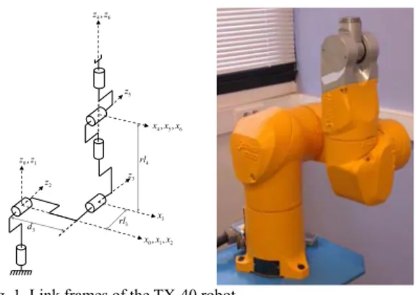
Fig. 1. Link frames of the TX-40 robot

2 2 1 1,1 1 1,n n τ τ 2 2 n 1 n 1,n 1 n 1 n 1,n n n n ,n n τ τ τ Y W χ ... W χ ... Y W χ W χ Y W χ                     (22) where the term YjWτj , jχj ... Wτj ,nχn  j is the

norm of the error on the estimation of the joint j torque. Thus, minimizing the squared norm of is a stepwise

coupled minimization of each squared norm of error j

  , starting from the parameters _{χ . The squared norm}n n 2

 

in (22) contributes giving a good estimation of _χn_{, then the}

squared norm n 1 2



  _{contributes giving a good estimation} of the parameters _χn 1 _{, etc.}

Considering now the PIM, it can be directly observed that the observation matrix of (21) doesn’t have a block-triangular form and that the squared norm of the error _Pis:

 2   1 1  n n 2

P YP W χP ... W χP (23)

As the wrist links are lighter, the contribution of the wrist actuators to the total robot power is quite small with regards to the shoulder power, i.e. for a 6 DOF robot,

4 4 5 5 6 6 1 1 2 2 3 3

P P P P P P

W χ W χ W χ W χ W χ W χ .

Thus, the LS solution of (21) may lead to a poor estimation of the wrist parameters.

Minimizing (23) using the PIM-WLS procedure should be compared with the IDIM-WLS procedure using only the joint 1 data in (22), i.e. the squared norm of the error for joint 1,

 

1 2  1 1,1 1  1,n n 2

τ τ

Y W χ ... W χ . (24)

This result will be shown in the next section. This problem can be avoided by creating a block-triangular regressor thanks to the use of optimal experimental trajectories. Using the property of matrices dh mentioned in section III for a n-DOF industrial serial robot, the block-triangular form of W can be obtained by carrying out at least

n different types of trajectories that cancels some terms of

W:

1. Trajectories with all joints moving altogether

2. Trajectories with joint 1 fixed (q1 0), all the other joints (from 2 to n) moving altogether

3. Trajectories with joints 1 and 2 fixed (q₁q₂ 0), all the other joints (from 3 to n) moving altogether

…

n. Trajectories with joints 1 to n–1 fixed (q₁q₂ ...



q_{n 1}0), joint n moving only.

Using these trajectories, the observation matrix built with the PIM takes block-triangular form. In the next section, the

PIM-WLS identification procedure is compared with the

IDIM-WLS procedure in order to show its efficiency.

V. CASE STUDY A. Description of the TX 40 kinematics

The Stäubli TX-40 robot (Fig. 1) has a serial structure with six rotational joints. Its kinematics is defined using the modified Denavit and Hartenberg notation (MDH) [15]. In this notation, the link j fixed frame is defined such that the

j

z axis is taken along joint j axis and the x axis is along _j

the common normal between z and _j z_{j 1}_ (Fig. 1). The geometric parameters defining the robot frames are given in Table 1. The payload is denoted as the link 7. The parameter

0

j

  , means that joint j is rotational, _j and d_j

parameterize the angle and distance between z_{j 1}_ and z _j

along x_{j 1}_ , respectively, whereas _j and r parameterize _j

the angle and distance between xj 1 and x along j z , j

respectively. For link 7, _j 2 means that the link 7 is fixed on the link 6. Since all the joints are rotational then _j

is the position variable qj of joint j .

The TX-40 robot is characterized by a coupling between the joints 5 and 6 such that:

           _ _          5 5 5 6 6 6 6 qr N 45 0 q qr N 32 N 32 q     ,       _ _     _ _           5 5 6 6 c ₅ ₆ r 6 c r N N 0 N (25)

where qr _jis the velocity of the rotor of motor j, q_jis the velocity of joint j, Nj is the transmission gain ratio of axis j,

τcj is the motor torque of joint j, taking into account the

coupling effect on the motor side, τrj is the electro-magnetic

torque of motor j.

TABLEI

GEOMETRIC PARAMETERS OF THE TX-40 ROBOT WITH THE PAYLOAD

j j j dj j rj 1 0 0 0 q1 0 2 0  0 q2-/2 0 3 0 0 d3 = 0.225 m q3+/2 rl3 = 0.035 m 4 0  0 q4 rl4 = 0.225 m 5 0  0 q5 0 6 0  0 q6 0 7 2 0 0 0 0

(6)

The coupling between joints 5 and 6 also adds the effect of the inertia of rotor 6 and new viscous and Coulomb friction parameters Fvm6and Fcm6 , to both τc5 and τc6.

It is possible to write: sign( ) c₅ 5 Ia q66  Fvm q66 Fcm 6 q6 and





sign( + ) sign( ) _c₆ ₆ Ia q₆₅ Fvm q₆₅ Fcm₆ q q₅ ₆  q₆

where τj already contains the terms

 

j j j j j j

( Ia q Fv q Fc sign( q ))  , for j=5 and 6 respectively,

with  2  2

5 5 5 6 6

Ia N Ja _{N Ja and}  2

6 6 6

Ia N Ja (26)

Jaj is the moment of inertia ofrotor j.

(26) is introduced into (4), (8) to obtain the IDIM and PIM.

B. Identification results

In this section, the identification procedure using PIM is compared with the usual method using IDIM. Three cases will be tested:

- Case 1: the robot dynamic parameters are identified with usual IDIM-WLS, using a single exciting trajectory with all joints moving simultaneously;

- Case 2: the robot dynamic parameters are identified with usual IDIM-WLS, using optimal trajectories presented in

section IV.B;

- Case 3: the robot dynamic parameters are identified with

PIM-WLS using the same trajectory as for Case 1;

- Case 4: the robot dynamic parameters are identified with

PIM-WLS using the same trajectory as for Case 2.

Some small parameters remain poorly identifiable because they have no significant contribution in the joint torques. These parameters have no significant estimations and can be cancelled in order to simplify the dynamic model. Thus parameters such that the relative standard deviation %_ˆ_ri is

too high are cancelled to keep a set of essential parameters of a simplified dynamic model with a good accuracy [16]. The essential parameters are calculated using an iterative

TABLEIII

QUALITY OF IDENTIFICATION.

Case 1 Case 2 Case 3 Case 4

Rel. Err. normˆ / Y 0.077358 0,0821229 0,0689218 0,0670227

mean(%ei1) — — 119.09 22.89

mean(%ei2) — — 131.97 21.70

ˆ Y Wˆ

    is the minimal norm of error.

TABLEII

IDENTIFIED DYNAMIC PARAMETERS.

Case 1 Case 2 Case 3 Case 4

Par. Values %ˆri Values %ˆri Values %ˆri %ei1 %ei2 Values %ˆri %ei %ei2

zz1r 1,29e+00 0,45 1,27e+00 0,36 1,18e+00 2,40 8,53 7,09 1,24e+00 1,84 3,88 2,36

fv1 6,90e+00 0,78 6,90e+00 0,58 7,98e+00 1,73 15,65 15,65 5,33e+00 4,54 22,75 22,75

fs1 6,71e+00 2,37 6,72e+00 1,76 — — — — 1,59e+01 6,45 136,96 136,61

xx2r -4,57e-01 2,02 -4,84e-01 1,44 -4,68e-01 6,26 2,41 3,31 -4,22e-01 9,19 7,66 12,81

xy2 — — — — -1,06e-01 21,66 — — — — — —

xz2r -1,35e-01 4,3 -1,45e-01 3,03 -1,32e-01 9,45 2,22 8,97 -1,22e-01 12,79 9,63 15,86

zz2r 1,06e+00 0,57 1,06e+00 0,31 1,24e+00 1,97 16,98 16,98 1,09e+00 1,25 2,83 2,83

mx2r 2,22e+00 0,52 2,21e+00 0,27 2,02e+00 1,95 9,01 8,60 2,18e+00 0,98 1,8 1,36

fv2 4,54e+00 1,33 4,45e+00 0,72 1,42e+00 26,46 68,72 68,09 4,28e+00 3,19 5,73 3,82

fs2 8,11e+00 1,83 7,87e+00 0,97 2,80e+01 7,18 245,25 255,78 8,25e+00 6,68 1,73 4,83

xx3r — — 9,49e-02 7,62 — — — — — — — —

xz3 — — — — 0,093 23,48 — — — — — —

yz3 — — — — 0,225 10,06 — — — — — —

zz3r 1,39e-01 3,7 1,46e-01 1,81 2,70e-01 10,47 94,24 84,93 1,57e-01 6,56 12,95 7,53

my3r -6,30e-01 1,53 -6,07e-01 0,79 — — — — -6,10e-01 1,5 3,17 0,49

ia3 8,27e-02 5,83 8,74e-02 2,85 — — — — 7,54e-02 12,88 8,83 13,73

fv3 1,73e+00 2,61 1,60e+00 1,19 — — — — 1,32e+00 3,47 23,7 17,5

fs3 6,30e+00 2,4 6,30e+00 1,03 2,08e+01 3,35 230,16 230,16 7,50e+00 3,36 19,05 19,05

xy4 — — — — -0,1 11,09 — — — — — —

yz4 — — — — 0,0588 19,79 — — — — — —

zz4r — — — — — — — — 3,72e-02 4,48 — —

mx4 — — — — — — — — -4,27e-02 12,67 — —

ia4 — — 3,51e-02 3,81 — — — — — — — —

fv4 9,15e-01 4,79 8,51e-01 1,78 8,56e-01 9,90 6,45 0,59 7,34e-01 3,02 19,78 13,75

fs4 2,40e+00 6,87 2,55e+00 2,31 — — — — 3,05e+00 4,56 27,08 19,61

yz5 — — — — 0,0561 17,15 — — — — — —

ia5 5,44e-02 9,94 4,16e-02 4,84 1,96e-01 11,86 260,29 371,15 4,41e-02 7,47 18,93 6,01

fv5 1,60e+00 3,8 1,56e+00 1,42 3,02e+00 4,09 88,75 93,59 1,46e+00 3,08 8,75 6,41

fs5 3,37e+00 4,47 2,71e+00 1,92 — — — — 2,00e+00 9,54 40,65 26,2

xy6 — — — — 0,0182 21,67 — — — — — — xz6 — — — — — — — — -2,54e-03 22,05 — — zz6 — — — — -0,026 11,49 — — — — — — mx6 — — — — 0,055 17,75 — — -2,53e-02 10,48 — — my6 — — — — 0,0547 19,12 — — — — — — ia6 — — 1,09e-02 4,43 — — — — 9,99e-03 2,76 — 8,35

fv6 5,81e-01 4,91 5,13e-01 1,69 1,29e+00 6,36 122,03 151,46 4,01e-01 1,81 30,98 21,83

fs6 1,96e+00 7,72 1,83e+00 2,68 -8,58e+00 11,04 537,76 568,85 2,63e+00 2,97 34,18 43,72

fvm6 5,19e-01 4,59 4,92e-01 1,69 8,08e-01 8,09 55,68 64,23 3,39e-01 3,05 34,68 31,1

fsm6 1,85e+00 7,76 1,53e+00 3,19 -2,97e+00 32,24 260,54 294,12 2,79e+00 4,41 50,81 82,35

i

ˆ



 is the standard deviation and

ri

ˆ

%_ its relative value (%). %ei1 is the relative difference (%) between the parameters identified in Case 1 and those

(7)

0 1 2 3 4 5 6 7 −80 −60 −40 −20 0 20 40 60 80 Time (s) Motor torque (N × m) Joint 1 Measure=Y Estimation=W X Error=Y−W X

Relative norm of error: ||ρ||/||Y||=0.0713

0 1 2 3 4 5 6 7 −100 −80 −60 −40 −20 0 20 40 60 Time (s) Motor torque (N × m) Joint 2 Measure=Y Estimation=W X Error=Y−W X

0 1 2 3 4 5 6 7 −30 −20 −10 0 10 20 30 Time (s) Motor torque (N × m) Joint 3 Measure=Y Estimation=W X Error=Y−W X

0 1 2 3 4 5 6 7 −10 −8 −6 −4 −2 0 2 4 6 8 10 Time (s) Motor torque (N × m) Joint 4 Measure=Y Estimation=W X Error=Y−W X

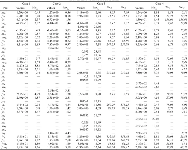
Fig. 2. Measured and reconstructed torques of the TX-40 with the parameters identified in Case 2.

0 1 2 3 4 5 6 7 −100 −80 −60 −40 −20 0 20 40 60 80 Time (s) Motor torque (N × m) Joint 2 Measure=Y Estimation=W X Error=Y−W X

0 1 2 3 4 5 6 7 −20 −15 −10 −5 0 5 10 15 Time (s) Motor torque (N × m) Joint 4 Measure=Y Estimation=W X Error=Y−W X

0 1 2 3 4 5 6 7 −30 −20 −10 0 10 20 30 40 Time (s) Motor torque (N × m) Joint 5 Measure=Y Estimation=W X Error=Y−W X

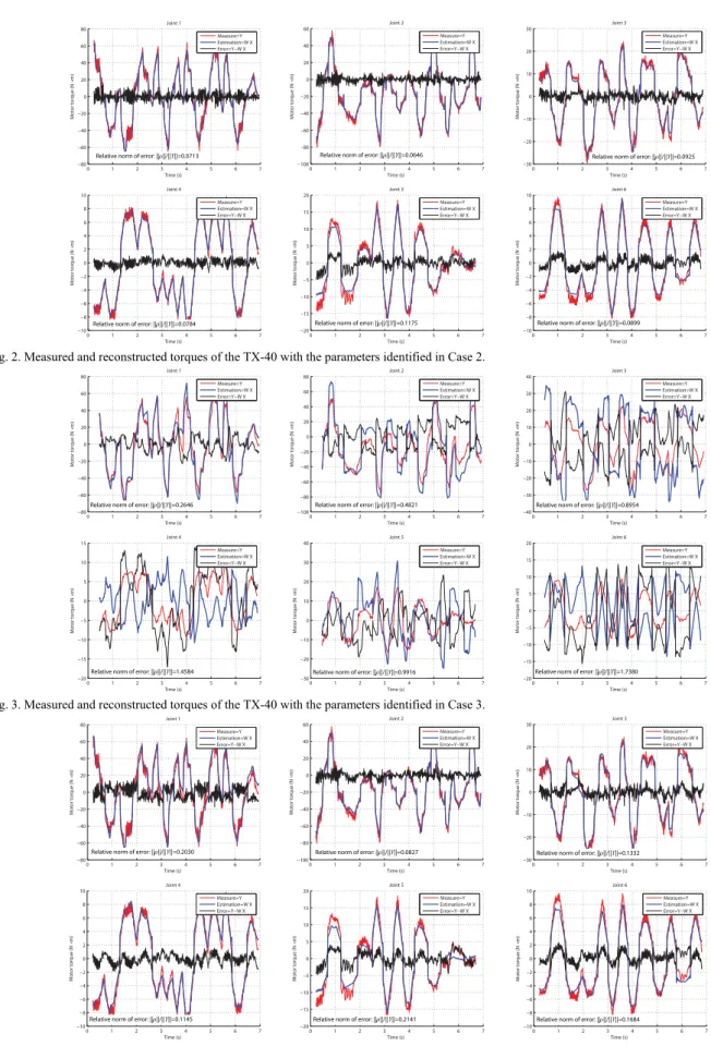
Fig. 3. Measured and reconstructed torques of the TX-40 with the parameters identified in Case 3.

0 1 2 3 4 5 6 7 −100 −80 −60 −40 −20 0 20 40 60 Time (s) Motor torque (N × m) Joint 2 Measure=Y Estimation=W X Error=Y−W X

0 1 2 3 4 5 6 7 −30 −20 −10 0 10 20 30 Time (s) Motor torque (N × m) Joint 3 Measure=Y Estimation=W X Error=Y−W X

(8)

TABLEIV

QUALITY OF TORQUE RECONSTRUCTION.

Case 1 Case 2 Case 3 Case 4 Case 5

Rel. Err. norm __{ˆ / Y} 0.0726 0.0765 0.5346 0.1545 0.7485

procedure starting from the base parameters estimation. At each step the base parameter which has the largest relative standard deviation is cancelled. A new LS parameter estimation of the simplified model is carried out with new relative error standard deviation %_ˆ_ri. The procedure ends

when _ _  _

ri ri

ˆ ˆ

max(% ) / min(% ) r , where r is a ratio

ideally chosen between 10 and 30 depending on the level of perturbation in Y and W. Here, for all identification procedures, r is fixed to 20.

The obtained results are shown in Table 2. The parameters with the subscript R stand for the regrouped parameters [3]. The results show that, in general, the parameters identified with PIM-WLS and optimized trajectories (Case 4) are closer to the parameters identified with IDIM-WLS (Cases 1 and 2). Some difference exists, but the parameters that have the largest differences %eij are

those that have the largest relative standard deviation. It can also be observed that a larger number of parameters can be estimated when IDIM-WLS uses the trajectories optimized for PIM-WLS (Case 2), compared with the IDIM-WLS results obtained with a single trajectory (Case 1).

Table 3 presents the mean of the relative differences %eij

between the parameter values estimated with PIM-WLS and

IDIM-WLS. For the parameters estimated in Case 4, the

mean of the difference with respect to those estimated in Cases 1 and 2 is stable and about 22%. For the parameters estimated in Case 3, this value is from 6 times higher.

The relative error norm that gives an estimation of the quality of the identification procedure is also shown in the Table 3. Both PIM-WLS methods have a good identification quality, i.e. the identified parameters well estimate the robot power. However, only the IDIM-WLS and PIM-WLS procedure with optimized trajectories can correctly estimate the input torques (Fig. 2, 3 and 4; the reconstructed torques for Case 1 are not shown because the curves are very similar to those of Case 2), even if IDIM-WLS shows better results.

Finally, a last IDIM-WLS procedure is carried out to identify the robot parameters using the equation of joint 1 only (denoted as Case 5). The relative norm of error for each case of identification is shown in Table 4. The results show that, as mentioned in section IV.B., the torques are poorly reconstructed using both PIM-WLS with a single trajectory and IDIM-WLS with the equations of joint 1 only, i.e. without the use of a block-triangular observation matrix.

Moreover, the quality of reconstruction is twice better with IDIM-WLS than with PIM-WLS. This can partially be explained by the fact that vector YP in (21) is correlated with

the observation matrix WP as they both depend of the

estimated values of q in which there is noise. A possible solution to this problem is to adapt the procedure DIDIM [17] to the PIM, as this procedure uses simulated values (without noise) of q . This is part of our future work.

VI. CONCLUSION

This paper dealt with the identification of robot inertial parameters using the power model. This method uses a model with symbolic expressions dramatically simpler to compute than those of the usual inverse dynamic identification model, was formerly applied for the identification of the dynamic parameters of a planar 2-DOF serial robot but failed when applied to a 6-DOF serial industrial robot. The causes of this failure are disclosed in the present paper. It is shown that it is necessary to create a block-triangular observation matrix via the use of optimized trajectories in order to correctly identify the wrist inertial parameters. If not, the identification fails to find the parameters that are able to correctly estimate the actuator torques. The method has been experimentally validated on a Stäubli TX-40 robot and the results shown that this method is efficient for identifying the dynamic parameters of a 6 DOF industrial robot.

REFERENCES

[1] M. Gautier, “Identification of robots dynamics”, Proc. IFAC Symp. on

Theory of Robots, Vienne, Austria, December 1986, p. 351-356. [2] C. Canudas de Wit and A. Aubin, “Parameters identification of robots

manipulators via sequential hybrid estimation algorithms”, Proc. IFAC

Congress, Tallin, 1990, pp. 178-183.

[3] M. Gautier and W. Khalil, “Direct calculation of minimum set of

inertial parameters of serial robots”, IEEE TRO, Vol. 6, No. 3, 1990.

[4] J. Hollerbach, W. Khalil and M. Gautier, “Model Identification”,

chapter 14 « Springer Handbook of Robotics », Springer, 2008.

[5] W. Khalil and E. Dombre, “Modeling, identification and control of

robots”, Hermes Penton London, 2002.

[6] P.K. Khosla and T. Kanade, “Parameter identification of robot

dynamics”, Proc. 24th_{IEEE CDC, 1985, p. 1754-1760.}

[7] Z. Lu, K.B. Shimoga and A. Goldenberg, “Experimental determination

of dynamic parameters of robotic arms”, Journal of Robotics Systems,

Vol. 10, N°8, 1993, p.1009-1029.

[8] M.Gautier,“Dynamic identification of robots with power model”,

Proc. IEEE Int. Conf. on Robotics and Automation, 1997, Albuquerque, New Mexico, April, pp. 1922-1927.

[9] R. Featherstone, D.E. Orin, “Dynamics”, chapter 2 in B. Siciliano and

O. Khatib. eds « Springer Handbook of Robotics », Springer, 2008.

[10] H. Mayeda, K. Yoshida and K. Osuka, “Base parameters of

manipulator dynamic models”, IEEE Trans. on Robotics and

Automation, Vol. RA-6(3), 1990, p. 312-321.

[11] M. Gautier, “Numerical calculation of the base inertial parameters”, Journal of Robotics Systems, Vol. 8, N°4, 1991, pp. 485-506. [12] P. Corke, “In situ measurement of robot motor electrical constants,”

Robotica, vol. 23, no. 14, pp.433–436, 1996.

[13] M. Gautier and S. Briot, “Global Identification of Drive Gains

Parameters of Robots Using a Known Payload”, Proceedings of the

2012 International Conference on Robotics and Automation (ICRA 2012), May 14-18, 2012, Saint Paul, MI, USA.

[14] F. Reyes and R. Kelly, “Experimental Evaluation of Identifiation

Schemes on a Direct Drive Robot,” Robotica, 1997, Vol. 15, pp.

563-571.

[15] W. Khalil and J.F. Kleinfinger, “A new geometric notation for open

and closed loop robots”, Proceedings of the IEEE International

Conference on Robotics and Automation, 1986, San Francisco.

[16] C.M. Pham, M. Gautier, “Essential parameters of robots” Proceedings

of the 30th Conference on Decision and Control, 1991, Brighton, England, December, pp. 2769-2774.

[17] M. Gautier, A. Janot and P.O. Vandanjon, “DIDIM: A New Method for the Dynamic Identification of Robots from only Torque Data,” Proc. ICRA 2008, Pasadena, USA.