Automated performance deviation detection across software versions releases

(1)

Titre:

Title

:

Automated performance deviation detection across software

versions releases

Auteurs:

Authors

:

Abderrahmane Benbachir, Isnaldo Francisco De Melo, Michel R.

Dagenais et Bram Adams

Date: 2017

Type:

Communication de conférence / Conference or workshop item

Référence:

Citation

:

Benbachir, A., Melo, I. F. D., Dagenais, M. R. & Adams, B. (2017, juillet). Automated performance deviation detection across software versions releases. Communication écrite présentée à 2017 IEEE International Conference on Software Quality, Reliability and Security (QRS), Prague, Czech Republic (8 pages). doi:10.1109/qrs.2017.55

Document en libre accès dans PolyPublie

Open Access document in PolyPublie URL de PolyPublie:

PolyPublie URL: https://publications.polymtl.ca/2977/

Version: Version finale avant publication / Accepted version_{Révisé par les pairs / Refereed} Conditions d’utilisation:

Document publié chez l’éditeur officiel

Document issued by the official publisher Nom de la conférence:

Conference Name: 2017 IEEE International Conference on Software Quality, Reliability and Security (QRS)

Date et lieu:

Date and Location: 2017-07-25 - 2017-07-29, Prague, Czech Republic

Maison d’édition:

Publisher: IEEE

URL officiel:

Official URL: https://doi.org/10.1109/qrs.2017.55

Mention légale:

Legal notice:

reprinting/republishing this material for advertising or promotional purposes, creating new collective works, for resale or redistribution to servers or lists, or reuse of any copyrighted component of this work in other works.

(2)

Ce fichier a été téléchargé à partir de PolyPublie, le dépôt institutionnel de Polytechnique Montréal

This file has been downloaded from PolyPublie, the institutional repository of Polytechnique Montréal

(3)

Automated Performance Deviation Detection Across

Software Versions Releases

Abderrahmane Benbachir∗, Isnaldo Francisco De Melo jr†, Michel Dagenais‡and Bram Adams§

Department of Computer and Software Engineering, Polytechnique Montreal, Quebec, Canada

Email:{∗abderrahmane.benbachir, †isnaldo-francisco.de-melo-junior, ‡michel.dagenais, §bram.adams}@polymtl.ca

Abstract—Performance is an important aspect and critical

requirement in multi-process software architecture systems such as Google Chrome. While interacting closely with members of the Google Chrome engineering team, we observed that they face a major challenge in detecting performance deviations between releases, because of their very high release frequency and therefore limited amount of data on each. This paper describes a deep analysis on the data distributions followed by a comparative approach using median based confidence interval for software evaluation. This technique is capable of detecting performance related deviations. It is substantially different from the standard confidence interval, in that it can be used in the presence of outliers and random external influences since the median is less influenced by them. We conducted a bottom-up analysis, using stack traces in a very large pool of releases. The results show that our approach can accurately localize performance deviations at a function-level granularity, using a very small number of trace samples, nearby 5 runs.

I. INTRODUCTION

One of the prevailing metrics for software product quality evaluation is repeatability and accuracy of subsequent exe-cutions. As the complexity of software increases, along with user expectations and features, it is evermore necessary to reduce the perceivable performance issues. From an end user’s perspective, performance is tightly related to the software correctness and interactive responsiveness. Failing on either of those fronts may lead the customers to opt for a competitor’s better-performing product. Also, on more critical systems, a slow response from the software can result in taking incorrect decisions, for instance during a critical medical operation.

A multi-process software such as the Chromium browser (the open-source web browser upon which Google Chrome is built), has a large and increasing number of community-contributed code. To insure the high quality of such modern software systems, code review with testing and debugging remain the most commonly used techniques. Chromium uses an open source Python-based continuous integration testing framework known as Buildbot. Against every build, Chromium runs a series of performance tests, monitored by the Perf Sheriff tool for regression purposes. However, given a limited set of resources and time before each software release, in-house testing and debugging becomes insufﬁcient to ensure high quality. In development environments, testing typically covers only a fraction of the use cases being deﬁned by developers within the testing frameworks [1].

In Google Chromium, performance is an important aspect and a critical requirement. Therefore, many tools have been developed for diagnosing performance problems. However, it

still is a very hard task even for highly experienced developers. Performance bugs are very different and require considerable attention; it may involve changes to a large portion of the code, which might result in adding more artifacts to the software.

Tracing tools provide the ability to record events while the software executes normally on the system. Those events will have three main characteristics: a timestamp, a type and a payload. Therefore, tracing tools are appropriate for the accurate detection of performance problems. Any undesirable inﬂuence of the tracer on the system under test is called over-head. Modern tracers are now able to achieve low overhead, and hence, can be used on real production systems to track sporadic bugs.

The Trace Event Proﬁling Tool is the userspace tracing framework provided by the Chromium Project. It allows recording activity in Chrome’s processes. Tracing is achieved by recording the C++ or JavaScript methods signatures in a de-tailed chronological view. Nevertheless, the recorded process generates a large amount of information, which can be used, through a mining process, to track performance bottlenecks, as well as slow executions.

While interacting closely with members of the Google Chrome engineering team, we discovered that their interest is not just in detecting performance degradation between releases, but also in detecting performance improvements induced through micro-optimizations. In this work, we propose a median-based confidence interval technique, which is an enhancement of the traditional statistical technique known as the confidence interval (CI). It was applied for performance deviation detection across many releases. As a consequence, the finding raises the possibility of using the comparative confidence interval metrics as a regression technique. Please note that we use in this paper the acronym CI to refer to the Confidence Interval, not Continuous Integration as is often the case in the DevOps community.

The issues discussed above form a base for the followings questions to be answered in this work;

• RQ 1: Can our approach detect performance deviations? • RQ 2: How much tracing data is required for the

detec-tion?

The remainder of this paper is organized as follows. Section II discusses related work. Section III describes the approach em-ployed collecting execution traces and detecting performance deviations using the conﬁdence interval technique. Section IV describes the evaluation steps applied on Chromium Browser. Section V summarizes the results of this study and answers the

(4)

research questions. Section VI introduces a short discussion about our ﬁndings and outlines threats to validity. Finally, Section VII concludes the paper with future directions.

II. RELATEDWORK

There are many related studies which intend to detect and diagnose performance variations by comparing two different executions. This paper presents a methodology for localizing performance deviations across large groups of releases without relying on comparisons techniques. Most of the work in the area of regression detection focuses on performance anomalies in load tests.

Nguyen et al. [2] carried out a series of researches on per-formance regressions. They recommend to leverage statistical control strategies, for example control graphs, to distinguish performance regressions. They create a control graph for each performance counter and analyze the infringement proportion of a similar performance counter in the target software version. The work of Nguyen et al. is similar to ours, we both use a dynamic analysis approach for software evaluation, and we use statistical techniques for detecting performance regressions. Despite that, Nguyen et al. performed regression tests to collect performance counters; such an approach is limited because it cannot guarantee the full test coverage of the source code. The main difference in the statistical approach used by Nguyen and our approach is the detection scaling. Control chart techniques are limited to detect regressions between only two versions at a time, our work uses a conﬁdence interval technique that can indeﬁnitely scale to detect regressions on a very large group of versions.

Heger et al. [3] present an approach to integrate performance regression root cause analysis into development environments. Developers are provided with visual graphics that help them identify methods causing the regression. The approach ducts unit tests to collect performance measurements and con-sequently provides no feedback on the performance expected in realistic environments.

There are also other approaches to detect variations during performance monitoring of production systems. Doray et al. [4] propose a new tool, TraceCompare, that facilitates perfor-mance variation detection between multiple executions of the same task. They used the Enhanced Calling Tree (ECCT) as a data structure to store trace executions and to represent the performance characteristics of task executions. Doray’s work allows effective comparisons between groups of executions of the same task. However, such work has not yet been extended for comparing between different task versions.

III. APPROACH

In this section, we present our approach for detecting performance deviations between consecutive releases. Every subsection relates to a stage in our approach, as shown in Figure 1. This section gives a complete overview of the trace collection approach and the statistical technique used during the detection process.

A. Trace Collection

The Chromium trace framework provides several trac-ing mechanisms such as: Function Tractrac-ing, Asynchronous Events and Counters. Function tracing is widely used by Chromium developers and it provides C++ macros arranged as TRACE EVENT to record begin and end of function calls. However, this technique has a disadvantage, since developers have to manually instrument the desired functions.

The engineering team at Google Chrome intends to implement a Dynamic Race Detector, which is a tool for compile-time instrumentation that has been integrated into the LLVM compiler [5]. This compiler-based instrumentation will pro-vide the ability to enable dynamic tracing everywhere inside Chromium.

In our work, we focused on trace events emitted by Function Tracing trace-points, and as a result we got hierarchical stack traces of function calls. These function calls represent the main tasks occurring inside the browser.

B. Preprocess Traces

The Trace Event Format is the trace data representation that is created by Chromium while tracing is enabled. It’s a JSON format that contains a list of different event types such as: Duration Events, Complete Events, Async Events, Flow Events and Counter Events. [6]

Catapult is an open-source project and home for several performance tools that span gathering, displaying and analyzing performance data for the Chromium project. To import traces from the JSON format into call stacks objects, we used the Trace-Viewer importer module based in the Catapult project. Given the very large size of data traces, we ﬁlter call stacks and keep only those within the main thread responsible for rendering web pages. This thread is known as CrRendererMain, from the Renderer process.

Figure 2: Processing call stacks for self-time metric The performance counters collected and used for deviation detection are CPU proﬁles. CPU proﬁles show where the execution time is spent within the instrumented function, and functions within children; this information is extracted as self-time and total-self-time, as shown in Figure 2.

The Self-time is deﬁned as the amount of time spent in a speciﬁc program unit. For instance, the self-time for a source

(5)

Trace Collection Preprocess traces Compute Interval_Estimation Detect Deviations

Userspace Traces Filter Callstacks

Figure 1: An Overview of Our Approach. line indicates the time spent on this speciﬁc source line by

the application. The Self-time offers a considerable level of insight into the effect that a function has on the program. Examining the effect of a single unit is otherwise called bottom-up analysis.

The Total-time refers to the aggregated time incurred by a program unit. For functions, the total-time involves the self-time of the function itself and the self-self-time of the entire dynamic call tree of functions that were called from that function. The total-time also empowers an advanced level of comprehension on the utilization of time in the application. Examining the effect of this metric is otherwise called top-down analysis [7].

As part of this work, we will mainly focus on the self-time metric to detect performance deviations at function-level granularity.

C. Compute Interval Estimation

The motivation behind taking a random sample from a group or population, and computing statistical parameters such as mean from the data, is to approximate the mean of the population.

In statistics, estimating the underlying population value is always an issue. An Interval Estimation addresses this issue by providing a range of values which act as good estimates of the population parameter of interest.

A Confidence Interval (CI) delivers a move from a solitary value estimate, (for example, the sample mean, variation between sample mean and so on) to a scope of qualities that are thought to be acceptable for the population. The width of a confidence interval in light of a sample measurement is substantially dependent on its Standard Error (SE), and consequently on both the sample estimate and the standard deviation. It likewise relies upon the level of ”confidence” that we need to connect with the subsequent interval [8].

In this step, we compute the conﬁdence interval (conﬁdence level of 95%) using the self-time of each function retrieved from collected stack traces.

Before computing conﬁdence intervals, we must check the distribution properties within the data-set.

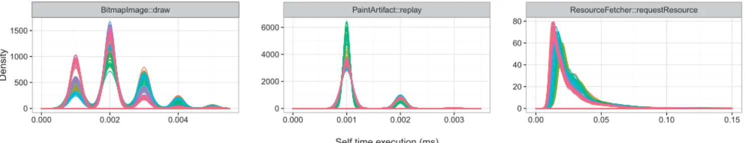
In the software system that we study, only 8% of the studied runs have unimodal distribution, with one clear peak. In fact, we affirm that these runs are normal as confirmed by Shapiro-Wilk tests (p >0.05). However, in the 92% of the remaining data, as shown in Figure 3, we discern three types of recurring distributions that are most present. Each color is related to a specific Chromium release, see Appendix A for more details.

This low level of normality in our data-set was expected,

especially when dealing with real world experiments which contain non-deterministic events.

In the multimodal distribution, we noticed that it contains alternately tall and short waves. This often results from a faulty measurement, a rounding error or a version of the plateau distribution. For example, a time duration rounded off to the nearest 0.3 ms would show a multimodal shape if the bar width for the histogram was 0.2 ms. We analysed most of the multimodal runs from the data-set. We found that they all have small measurement values, the smallest precision measurement that we can get is 1 microsecond. We explored the Chromium source code; we found out that all event timestamps emitted by the Chromium tracer framework are effectively limited to microsecond granularity [9]. The right-skewed distribution is similar to a normal distribution but asymmetrical. The distributions peak is off center toward the limit, and a tail stretches away from it toward the right.

The majority of the runs in our data-set have skewed and bi-modal distribution, the bi-modal distribution is similar to the middle chart in Figure 3.

Bi-modal runs have two different modes; they appear as distinct peaks, the local high points of the chart. This distribution exposes the existence of two different populations, both of them can be represented as uni-modal distributions. When dealing with such cases, using the median over the mean estimator produces more accurate results.

Given the different shapes of the distributions, no single estimator is always optimal. While the mean is optimal for low skew data since the distribution is normal, the median is clearly preferable for bi-modal and skewed data. With overly erroneous or generally difﬁcult data, the median might be a favorable choice, instead of the mean, as an estimation of central tendency, and used with nonparametric procedures for evaluation.

David Olive [10] in the Department of Mathematics at Southern Illinois University, proposed an alternative approach for computing CI using the median metric.

Confidence Interval for the median. As Olive states in his literature [10], a benefit of his confidence interval for the median is the fact that it gives a straight forward, numerical means of distinguishing circumstances where the data val-ues require painstaking, graphical evaluation. Specifically, he supports comparing the conventional confidence interval for the mean against his confidence interval for the median, if these intervals are markedly different, it is worth investigating to understand why. The main concept here is that under the ”standard” working assumptions (i.e., distributional symmetry

(6)

BitmapImage::draw 0 500 1000 1500 0.000 0.002 0.004 Density Multimodal Distribution PaintArtifact::replay 0 2000 4000 6000 0.000 0.001 0.002 0.003

Self time execution (ms) Bimodal Distribution ResourceFetcher::requestResource 0 20 40 60 80 0.00 0.05 0.10 0.15 Skewed Distribution

Figure 3: Three Shapes Distribution and estimated normality) the mean and the median ought to

be almost identical. In the event that they differ, it presumably implies a tampering of the working assumptions, because of exceptions in the data, declared distributional asymmetry, or different less frequently occurring instances like strongly multimodal data distributions or coarse quantization.

The reliability is an important aspect of using median instead of mean, even in the presence of outliers or non-deterministic events that might bias the data. While it is impossible to predict the perturbing events, it is possible to avoid them by using median-based analysis.

D. Detect Deviations

In Figure 6, we can easily localize the deviation happening at version 56.0.2910.0, because it is visually possible to make this distinction when such large deviations happen.

In the increasingly common case where we have a lot of numerical variables to consider, it may be undesirable or infeasible to examine them all graphically. Statistical tests to measure the difference between two conﬁdence intervals, like the one described by [11] may be automated and used to point us to speciﬁc deviations.

Figure 4: Statistical signiﬁcance between two conﬁdence in-tervals.

In order to automatically compute theses deviations, two requirement are essentials :

• The two medians are signiﬁcantly different (α = 0.05) when the CI for the difference between the two group medians does not contain zero.

• The two medians do not have overlapping conﬁdence intervals if the lower bound of the CI for the greater median is greater than the upper bound of the CI for the smaller median.

If a CI overlap is present, it is not possible to determine a difference with certainty. Since there is no CI gap, a signiﬁcant difference can be tracked as explained in Figure 4.

Figure 5: Comparing two confidence intervals In order to compare two confidence intervals, we must con-sider two aspects: statistical significance and calculated over-lap. Figure 5 shows two cases, comparing two CI, overlap and gap.

IV. EVALUATION

The data-set used in the work has been extracted using the chromium-browser-snapshots repository. With the repository API, we fetched all the builds meta-data and we stored them locally for offline processing. Each build entry contains five fields: build-number, version-number, date, git-commit-id, and media-link.

We ﬁlter the data-set to select only builds within the year 2016, we removed some builds that had the same version number and we only kept the latest ones. After this step, the data-set is reduced to 300 builds. From this data-set, we narrow it for only the latest 100 releases distributed in the last four months, consult Appendix A for more details about releases.

After downloading all building binaries the from Chromium repository, we started by running a basic workload on each release. This workload consists of rendering a regular web page 1_{. The scenario takes about two seconds to complete.}

When the workload is completed, we killed all chromium processes before running the next experiment.

Ahead of running the workloads on each release, we removed cache and conﬁgurations ﬁles that were stored by the previous

(7)

release; we also didn’t trace the ﬁrst run (cold-run), consider-ing chromium would need to do an initialization procedure before running the ﬁrst workload, to avoid noise that this behavior could possibly introduce.

On each run, we enabled Chromium userspace tracing using the ﬂag trace-startup. By the end of the experiment, a JSON ﬁle was created containing the execution trace of the workload. To prevent any disturbance, we avoided any activity while running the experiments.

For each release, we executed 50 times the same workload. As a result, we collected up to 50 Gigabytes of trace data.

V. RESULTS

This section explains the study results for the function tasks: Paint, V8.ScriptCompiler and GetRenderStyleForStrike. Due to space limitation, deviation detection ﬁndings of only some functions will be discussed. However, the reader is welcome to access the online repository [12] for more results related to other functions. This section also reveals the ﬁndings of the research questions investigated in the study.

RQ 1: Can our approach detect performance deviations ?

Our first research question is to find whether our approach is suitable to localize performance deviations across a large number of releases. We address this question by presenting some use cases, the first two cases identify many deviation types, where the last one exposes a case where median-based CI performed better than mean-based CI due to presence of non-deterministic events.

In the Paint task, as seen in Figure 6, we can clearly notice that a deviation happened between version 56.0.2909.0 and 56.0.2910.0, the duration difference is around 0.18 ms, which is a signiﬁcant gap. We obtained 0.18 ms when computing the median difference between the ﬁrst median 0.25 ms (56.0.2909.0) and the second one 0.07 ms (56.0.2910.0).

● ● ● ● ● ● ● ● ● ● ● ● ● 0.0 0.1 0.2 0.3 0.4 56.0.2900.056.0.2901.056.0.2904.056.0.2905.056.0.2906.056.0.2907.056.0.2909.056.0.2910.056.0.2911.056.0.2912.056.0.2913.056.0.2914.056.0.2915.0 Releases Self time (ms) C.I. type ● ● Mean Median

Figure 6: Paint conﬁdence intervals

In the V8.ScriptCompiler task, as seen in Figure 7, three deviations happened at 56.0.2904.0, 57.0.2927.0 and 57.0.2946.0. The ﬁrst two deviations were negative deviations,

because each one of them migrated to a higher value. Those kinds of deviations can be classified as regressions. When analyzing the third deviation, without taking into consideration the previous regressions, we might miss an important event. The third deviation has a fallback at the same level as before the first regression. This temporary deviation from the main line happened only for a certain period of time. This phenomena can be classified as a digression. Figure 8 is

● ● ● ● ● ● ● ● ● ● ● ● ● ● ● ● ● ● ● 0.2 0.4 0.6 56.0.2899.056.0.2900.056.0.2901.056.0.2904.056.0.2905.056.0.2906.056.0.2924.057.0.2925.057.0.2926.057.0.2927.057.0.2929.057.0.2930.057.0.2943.057.0.2944.057.0.2945.057.0.2946.057.0.2947.057.0.2948.057.0.2949.0 Releases Self time (ms) C.I. type ● ● Mean Median

Figure 7: V8.ScriptCompiler conﬁdence intervals

● ● ● ● ● ● ● ● ● ● ● ● ● ● ● ● ● ● ● ● 0.8 0.9 1.0 1.1 1.2 57.0.2929.057.0.2930.057.0.2932.057.0.2933.057.0.2934.057.0.2935.057.0.2936.057.0.2937.057.0.2938.057.0.2939.057.0.2940.057.0.2941.057.0.2942.057.0.2943.057.0.2944.057.0.2945.057.0.2946.057.0.2947.057.0.2948.057.0.2949.0 Releases Self time (ms) C.I. type ● ● Mean Median

Figure 8: GetRenderStyleForStrike conﬁdence intervals able to demonstrate a comparison of using mean and median based analysis. It is possible to verify that on mean-based analysis there is a deviation between releases 57.0.2939.0 and 57.0.2940.0, while it is not present on median-based curve. Instead, on mean-based analysis, there is a deviation between 57.0.2937.0 and 57.0.2938.0 releases which is not present on median-based curve.

In some cases. it is very difﬁcult to detect deviations by only relying on visual analysis. In such cases, we need an automated mechanism to get a precise result.

Automation can be reached by using the statistical tests and techniques discussed in section Approach Detect Deviations, which we computed between each consecutive intervals. For the interval comparison, we considered two essential

(8)

condi-tions: if a statistical test is signiﬁcant and no overlap is found, there is a deviation.

To summarize our results, we built a Deviation matrix shown in Figure 9.

The Deviation matrix is a visual tool that explains deviation types, since it visually emphasises them according to their properties. We can show several properties of the deviations on this matrix.

The deviations are represented as triangles with two directions. A negative deviation (regression) is represented as a standard triangle, and a positive deviation (improvement) is represented as a upside down triangle.

Also, in the Deviation matrix, the size of the shapes is related to the interval’s gap, a bigger gap results into a bigger shape. The squares represent non significant overlaps, and finally the dots represent significant overlaps.

The comparison takes in consideration two different aspects: statistical significance and calculated overlap. The triangles, therefore, are the cases for which the two essential conditions are fulfilled: statistical significance and clear Confidence In-terval gap.

RQ 2: How much tracing data is required for the detection ?

Our second research question is to ﬁnd how much trace data is needed for performance deviation detection. We address this question by presenting four different collected runs: 5, 10, 20 and 50 runs being collected. In Figure 10, we notice that after 5 trace runs, there is a tendency for the deviation to become more important, and intervals width becomes thinner as more runs are aggregated.

VI. DISCUSSION ANDTHREATS TOVALIDITY In this section, the results are discussed in details in relation to the research questions.

A. The Research Questions Revisited

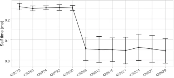
To better localize where the deviation happened in Figure 6 in release 56.0.2910.0, we did a source diff [13] between 56.0.2910.0 and the previous release which is 56.0.2909.0. We have found 363 commits, 63 of these commits have triggered 63 continuous integration builds, on which we applied our approach and we detected the deviation at build 429808 as presented in Figure 11. ● ● ● ● ● ● ● ● ● ● ● ● 0.0 0.1 0.2 429778 429780 429784 429792 429800 429808 429812 429815 429821 429824 429827 429829 Builds Self time (ms)

Figure 11: Paint conﬁdence intervals between continuous integration builds

In order to list the changes happening between 429800 and 429808, we applied a source diff [14] between commits that triggered theses builds. As a result, we found 8 commits summarized in Table I.

Table I: Changes that caused deviation in 429808

Commit Id Comment

0913b86 Add virtual tests for XHR with mojo-loading

d99d907 [DevTools] Remove handlers = browser from protocol def 4c2b05e preserve color space when copy nv12 textures is true 57d2116 [Extensions + Blink] Account for user gesture in v8 func 5516863 Enable compositing opaque ﬁxed position elements 65426ee Remove stl util´s deletion function use from storage c1d8671 [Devtools] Moved new timeline canvas context menu to c48291b cc/blimp: Add synchronization for scroll/scale state

We analysed the eight commits to find which one is responsible for the deviation, none of them did specific changes on the studied task (Paint). On the other hand, we could build each commit and run the experiments on theses builds. However, it would be a time consuming task, and it would not disclose which specific code change generated the deviation. Mainly because the functions changed on those commits were not instrumented, it would be hard to mine the source code to extract the involved nested function calls in this deviation. Consequently, expert input from Google developers is almost unavoidable.

The v8.ScriptCompiler has an interesting behaviour showing three deviations A closer examination on the Deviation Matrix shows a temporary deviation on the performance of this task. This deviation can be challenging to interpret precisely. This temporary regression could be explained by two possible causes. First, a change was added that lead to a performance degradation, this later was ﬁxed. Secondly, a code change was introduced and then later reverted to the previous state.

The two sides of both curves on ﬁgure 8 corroborate for a non presence of deviations. However, the behavior of the cen-ter (between 57.0.2938.0 and 57.0.2945.0) differ completely. The mean curve reveals an abrupt behavior, with smaller conﬁdence intervals and mean values which are approaching median values in the median curve.

Although mean and median are similar in terms of under-standing a tendency, in figure 8 they reveal opposite properties within their curves. The mean is not robust considering it has a disadvantage of being influenced by any single abnormal value, this can be verified by its curve, which has two drastic deviations at 57.0.2938.0 and 57.0.2945.0. The median is appropriated to distribution to our data-set and as consequence, its curve demonstrates strong stability toward outliers.

By analyzing Figures 6 and 7, we notice that the median-based intervals are small compared to mean-median-based intervals. Also, the Figure 8 shows mean-based sensitivity in the pres-ence of outliers, those results reveal the stability of using the median over the mean approach.

(9)

● ● FrameView::synchronizedPaint FrameView::updatePaintProperties GetRenderStyleForStrike Paint v8.callFunction v8.compile v8.run V8.ScriptCompiler 56.0.2900.056.0.2901.056.0.2904.056.0.2905.056.0.2906.056.0.2907.056.0.2909.056.0.2910.056.0.2911.056.0.2912.056.0.2913.056.0.2914.056.0.2915.056.0.2916.056.0.2917.056.0.2918.056.0.2919.056.0.2920.056.0.2921.056.0.2922.056.0.2924.057.0.2925.057.0.2926.057.0.2927.057.0.2929.057.0.2930.057.0.2932.057.0.2933.057.0.2934.057.0.2935.057.0.2936.057.0.2937.057.0.2938.057.0.2939.057.0.2940.057.0.2941.057.0.2942.057.0.2943.057.0.2944.057.0.2945.057.0.2946.057.0.2947.0 Releases Deviation size ● ● ● ● ● 0.00 0.05 0.10 0.15 0.20 ● Gap (Regression) Gap (Improvement) Not Signifi Overlap Significant Overlap

Figure 9: Deviation matrix : automatic deviation detection for studied functions and their relatives

● ● _● ● ● ● ● ● ● ● ● ● ● ● ● ● ● ● ● ● ● ● ● ● ● ● ● ● ● ● ● ● ● ● ● ● ● ● ● ● ● ● ● ● ● ● ● ● ● ● ● ● ● ● ● ● ● ● ● ● ● ● _● ● ● ● ● ● ● ● ● ● ● ● ● ● ● ● ● ● ● ● ● ● ● ● ● ● 05 runs 10 runs 20 runs 50 runs 0.00 0.25 0.50 0.75 0.00 0.25 0.50 0.75 56.0.2898.056.0.2899.056.0.2900.056.0.2901.056.0.2904.056.0.2905.056.0.2906.056.0.2907.056.0.2909.056.0.2910.056.0.2911.056.0.2912.056.0.2913.056.0.2914.056.0.2915.056.0.2916.056.0.2917.056.0.2918.056.0.2919.056.0.2920.056.0.2921.056.0.2922.056.0.2898.056.0.2899.056.0.2900.056.0.2901.056.0.2904.056.0.2905.056.0.2906.056.0.2907.056.0.2909.056.0.2910.056.0.2911.056.0.2912.056.0.2913.056.0.2914.056.0.2915.056.0.2916.056.0.2917.056.0.2918.056.0.2919.056.0.2920.056.0.2921.056.0.2922.0 Releases Self time (ms)

(10)

To define the statistically relevant deviations we still need help from experts. In order to allow an expert to use our current automation approach, a tuning phase for the detection is required. The main reason for this procedure is to determine the threshold between statistical significance and the practical significance. Due to the sample size effect, statistically significant differences can appear even with very small differences. This is in contrast to the practical significance, which is related to a specific domain. Hence, a professional practitioner direction for the system tests is still required [15].

The results observed in Figure 10 corroborate the Central Limit Theorem (CLT). This theorem asserts that the more we collect trace data, the more we get accurate results. Although, the more tracing data collected the more overhead it was added, consequently the overhead is directly proportional to the amount of data traced. Moreover, from Figure 10, the number of traces to keep the effectiveness of our method was ﬁve while keeping the overhead negligible, similar approach was also explored for logging in [16].

B. Threats to Validity

During the experiments, we used a Linux-based operating system machine with 4 GHz CPU speed and 32GB of RAM, which is not a common conﬁguration used among most users. The use of conﬁdence intervals on multi-modal distributions may lead to some inaccuracy in our results.

Since the conﬁdence Interval is an estimation, there is an approximation error which can lead to misleading performance deviations. Consequently, the performance detection has some restrictions for an accurate application. In this context though, since we don’t rely on just one estimation for deducing the performance behaviour, the approximations do not lead to a misinterpretation.

VII. CONCLUSION

A bottom-up analysis has been performed on collected stack traces, which led to the conclusion that interval estimation pro-vides a clear detection of performance deviations among many versions, even with limited data on each version. Furthermore, we used an improved conﬁdence interval that leads to more accurate results with very little tracing data. The previous work (speciﬁcally on performance debugging) typically focused on binary comparisons, limited between two versions. Our work extends beyond those previous limits and provides a graphical view, called Deviation matrix, that helps performance analysts effectively detect performance variations among many versions at the same time.

In the future, we plan to expand our investigation by analyzing deviations with different workloads and understand the factors causing regressions cases. In this work, we mostly focused on internal deviations caused by a change between different software versions. As future work, we also intend to analyze external deviations that might be caused by varying hardware properties, while keeping the same software version.

REFERENCES

[1] A. Barth, C. Jackson, C. Reis, T. Team et al., “The security architecture of the chromium browser,” Technical report, 2008.

[2] T. H. Nguyen, B. Adams, Z. M. Jiang, A. E. Hassan, M. Nasser, and P. Flora, “Automated detection of performance regressions using statis-tical process control techniques,” in Proceedings of the 3rd ACM/SPEC

International Conference on Performance Engineering. ACM, 2012, pp. 299–310.

[3] C. Heger, J. Happe, and R. Farahbod, “Automated root cause isolation of performance regressions during software development,” in

Proceed-ings of the 4th ACM/SPEC International Conference on Performance Engineering. ACM, 2013, pp. 27–38.

[4] F. Doray and M. Dagenais, “Diagnosing performance variations by comparing multi-level execution traces,” IEEE Transactions on Parallel

and Distributed Systems, 2016.

[5] K. Serebryany, A. Potapenko, T. Iskhodzhanov, and D. Vyukov, “Dy-namic race detection with llvm compiler,” in International Conference

on Runtime Veriﬁcation. Springer, 2011, pp. 110–114.

[6] N. Duca and D. Sinclair, “Trace event format,” January 2017. [On-line]. Available: https://docs.google.com/document/d/1CvAClvFfyA5R-PhYUmn5OOQtYMH4h6I0nSsKchNAySU

[7] Intel, “Self time and total time,” December 2016. [Online]. Available: https://software.intel.com/en-us/node/544070

[8] M. J. Gardner and D. G. Altman, “Conﬁdence intervals rather than p values: estimation rather than hypothesis testing.” Br Med J (Clin Res

Ed), vol. 292, no. 6522, pp. 746–750, 1986.

[9] Google, “Chromium source code repository,” December 2016. [Online]. Available: https://chromium.googlesource.com/chromium/src/ base/trace event/common/+/master/trace event common.h#58 [10] D. J. Olive, “A simple conﬁdence interval for the median,” Manuscript.

www.math.siu.edu/olive/ppmedci.pdf, 2005.

[11] C. University, “The root of the discrepancy,” December 2016. [Online]. Available: https://www.cscu.cornell.edu/news/statnews/Stnews73insert. pdf

[12] A. Benbachir, “Online repository,” January 2017. [Online]. Available: https://github.com/abenbachir/performance-deviations

[13] Google, “Chromium release diff 56.0.2909.0..56.0.2910.0,” December 2016. [Online]. Available: https://chromium.googlesource.com/ chromium/src/+log/56.0.2909.0..56.0.2910.0

[14] ——, “Chromium commit diff 5b9d52e..0913b86,” January 2017. [Online]. Available: https://chromium.googlesource.com/chromium/src/ +log/5b9d52e..0913b86?pretty=fuller

[15] M. Gall, “Figuring out the importance of research results: Statistical signiﬁcance versus practical signiﬁcance,” in annual meeting of the

American Educational Research Association, Seattle, WA, 2001.

[16] R. Ding, H. Zhou, J.-G. Lou, H. Zhang, Q. Lin, Q. Fu, D. Zhang, and T. Xie, “Log2: A cost-aware logging mechanism for performance diagnosis.” in USENIX Annual Technical Conference, 2015, pp. 139– 150.

APPENDIX

CHROMIUMRELEASESLEGEND 54.0.2837.0 54.0.2838.0 54.0.2839.0 54.0.2840.0 55.0.2841.0 55.0.2842.0 55.0.2843.0 55.0.2845.0 55.0.2846.0 55.0.2847.0 55.0.2848.0 55.0.2849.0 55.0.2850.0 55.0.2851.0 55.0.2853.0 55.0.2854.0 55.0.2855.0 55.0.2857.0 55.0.2858.0 55.0.2859.0 55.0.2861.0 55.0.2862.0 55.0.2863.0 55.0.2864.0 55.0.2865.0 55.0.2866.0 55.0.2867.0 55.0.2868.0 55.0.2869.0 55.0.2870.0 55.0.2871.0 55.0.2872.0 55.0.2873.0 55.0.2874.0 55.0.2875.0 55.0.2876.0 55.0.2877.0 55.0.2878.0 55.0.2879.0 55.0.2880.0 55.0.2881.0 55.0.2883.0 56.0.2884.0 56.0.2885.0 56.0.2886.0 56.0.2887.0 56.0.2888.0 56.0.2890.0 56.0.2891.0 56.0.2892.0 56.0.2894.0 56.0.2895.0 56.0.2896.0 56.0.2897.0 56.0.2898.0 56.0.2899.0 56.0.2900.0 56.0.2901.0 56.0.2904.0 56.0.2905.0 56.0.2906.0 56.0.2907.0 56.0.2909.0 56.0.2910.0 56.0.2911.0 56.0.2912.0 56.0.2913.0 56.0.2914.0 56.0.2915.0 56.0.2916.0 56.0.2917.0 56.0.2918.0 56.0.2919.0 56.0.2920.0 56.0.2921.0 56.0.2922.0 56.0.2924.0 57.0.2925.0 57.0.2926.0 57.0.2927.0 57.0.2929.0 57.0.2930.0 57.0.2932.0 57.0.2933.0 57.0.2934.0 57.0.2935.0 57.0.2936.0 57.0.2937.0 57.0.2938.0 57.0.2939.0 57.0.2940.0 57.0.2941.0 57.0.2942.0 57.0.2943.0 57.0.2944.0 57.0.2945.0 57.0.2946.0 57.0.2947.0 57.0.2948.0 57.0.2949.0