UNIVERSITÉ DU QUÉBEC
RÉPARTITION SPATIALE DU PICO-, DU NANO- ET DU
MICRO PHYTOPLANCTON DANS LE HAUT ARCTIQUE CANADIEN EN FIN DE SAISON ESTIVALE
MÉMOIRE PRÉSENTÉ À
L'UNIVERSITÉ DU QUÉBEC À RIMOUSKI comme exigence partielle du programme
de maîtrise en océanographie
PAR
GENEVIÈVE TREMBLAY
Avertissement
La diffusion de ce mémoire ou de cette thèse se fait dans le respect des droits de son auteur, qui a signé le formulaire « Autorisation de reproduire et de diffuser un rapport, un mémoire ou une thèse ». En signant ce formulaire, l’auteur concède à l’Université du Québec à Rimouski une licence non exclusive d’utilisation et de publication de la totalité ou d’une partie importante de son travail de recherche pour des fins pédagogiques et non commerciales. Plus précisément, l’auteur autorise l’Université du Québec à Rimouski à reproduire, diffuser, prêter, distribuer ou vendre des copies de son travail de recherche à des fins non commerciales sur quelque support que ce soit, y compris l’Internet. Cette licence et cette autorisation n’entraînent pas une renonciation de la part de l’auteur à ses droits moraux ni à ses droits de propriété intellectuelle. Sauf entente contraire, l’auteur conserve la liberté de diffuser et de commercialiser ou non ce travail dont il possède un exemplaire.
11
AVANT -PROPOS
Ce mémoire traite de la répartition spatiale de différentes classes de taille du phytoplancton marin dans le Haut Arctique Canadien en fin de saIson estivale. Il se compose d'une introduction générale, d'un chapitre central sous la forme d'un article scientifique et d'une conclusion générale. L'article sera soumis prochainement à une revue scientifique avec comité de lecture. Ce travail a été réalisé dans le cadre du Réseau de centres d'excellence du Canada ArcticNet. Les résultats préliminaires du chapitre central de ce mémoire ont été présentés à plusieurs rencontres scientifiques. En 2005, certains résultats ont été présentés sous forme d'affiche à la réunion annuelle de Québec-Océan ainsi qu'à la seconde réunion annuelle d'ArcticNet. En 2006, une partie de cette thèse a été vulgarisée pour une présentation grand public au Biodôme de Montréal et les résultats ont également été présentés oralement à l'Association francophone pour le savoir (ACF AS) et par affiche à la troisième réunion annuelle d'ArcticNet. Finalement, en 2007, les principaux résultats de cette étude ont fait l'objet d'une affiche présentée à la Gordon Research Conference - Polar Marine Science qui a eu lieu à Ventura en Californie.
l'aimerais tout d'abord remercier mes parents, ma sœur et mon frère ainsi que leurs petites familles respectives, pour leur appui soutenu tout au long de mes études, plus spécifiquement depuis les sept dernières années et malgré la distance, et de m'avoir aussi donné cette force et cette vigueur d'avancer dans la vie. Je vous remerCIe pour vos encouragements dans mes milliers de projets ... ou plutôt dans mes "plans de fous". Je
remercie aussi mes amis pour votre amitié et appui pendant toutes ces années d'études à l'extérieur.
Je tiens à remercier plus particulièrement mon directeur, le Dr Michel Poulin, et mon co-directeur de maîtrise, le professeur Michel Gosselin, qui ont contribué à la réussite de ce projet. Le Dr Poulin, du Musée canadien de la nature, m'a donné la chance de vivre une expérience unique dans l'Arctique. Merci pour cette belle opportunité d'étude et de travail de terrain. Merci aussi pour les corrections à mes nombreuses ébauches de documents scientifiques et surtout ta grande disponibilité et ton accessibilité tant sur le plan humain que professionnel. Le professeur Gosselin, de l'Institut des sciences de la mer de Rimouski, m'a permis de faire partie de son équipe. Merci pour les suggestions, commentaires et conseils scientifiques judicieux, j'ai beaucoup appris et je l'apprécie grandement. Un merci particulier au Dr Claude Belzile qui m'a donné un sérieux coup de main lors de la rédaction de mon article. l'aimerais aussi remercier la professeure Suzanne Roy, Mélanie Simard et Caroline Jose pour leur assistance technique ainsi que les professeurs Yves Gratton et Jean-Éric Tremblay qui m'ont fourni respectivement des données physiques du CTD et des éléments nutritifs.
Finalement, je tiens à remercier les organismes qui ont soutenu financièrement cette étude, soit le Conseil de recherches en sciences naturelles et en génie du Canada (CRSNG), le Musée canadien de la nature, le programme de formation scientifique dans le Nord du ministère des Affaires indiennes et du Nord, l'Institut des sciences de la mer de Rimouski
IV
(ISMER) et Québec-Océan. J'en profite aussi pour remercier les officiers de la Garde côtière canadienne et l'équipage du NGCC Amundsen pour leur support technique lors de la mission scientifique en mer de 2005.
RÉSUMÉ
Ce mémoire traite de la structure de taille des communautés phytoplanctoniques marines dans le Haut Arctique canadien à la fin d'une saison estivale. Ce mémoire a pour objectifs 1) de décrire la répartition spatiale du micro-, du nano- et du picophytoplancton dans les trois régions océanographiques du Haut Arctique canadien (la baie de Baffin, le Passage du nord-ouest et la mer de Beaufort), et 2) d'évaluer les variables environnementales gouvernant la répartition du phytoplancton. Une meilleure connaissance de l'état actuel des différents groupes phytoplanctoniques nous permettra de mieux prévoir la réponse du phytoplancton arctique à une réduction du couvert de glace, à un accroissement de la stratification de la colonne d'eau et à une augmentation de la température des eaux de surface.
Le microphytoplancton (20-200 !lm) et le nanophytoplancton (2-20 !lm) ont longtemps été reconnus comme les deux classes de tailles dominantes dans l'Arctique. Mais depuis les dernières avancées technologiques (e.g. la cytométrie en flux et la biologie moléculaire), certaines études ont démontré que l'Arctique supporte un réseau trophique microbien bien développé (e.g. Lovejoy et al. 2007) et que le picophytoplancton (0,2-2 !lm) domine la communauté phytoplanctonique à certaines périodes de l'année.
Dans l'ensemble, le Haut Arctique canadien est dominé à l'été par le picophytoplancton qui représente 76,2% de la communauté phytoplanctonique (pico-
+
VI
nano-+ microphytoplancton). L'abondance de ces cellules <2 !lm varie entre 150 et 18 400 cellules mr1• La biomasse du picophytoplancton représente aussi une fraction élevée de la chlorophylle a totale sur presque tout l'ensemble des stations du Haut Arctique canadien. La fraction du picophytoplancton est essentiellement composée de cellules eucaryotes alors que des picocyanobactéries ont été observées à quelques stations près des côtes dans la mer de Beaufort avec des abondances < 120 cellules mr1
• Ainsi les cellules picoeucaryotes sont une composante importante en terme d'abondance et de biomasse qui devrait être mise en évidence lors d'études d'impact sur les réseaux trophiques supérieurs.
En été, le nanophytoplancton et le microphytoplancton sont moins abondants que le picophytoplancton dans le Haut Arctique canadien. Le nanophytoplancton et le microphytoplancton représentent respectivement 23,2% et 0,6% de la communauté phytoplanctonique. Significativement plus abondant dans la baie de Baffin qu'en mer de Beaufort, le nanophytoplancton semble avoir été avantagé par un mélange vertical résultant d'une faible intensité de stratification. Suite aux analyses microscopiques, la composition spécifique du nanophytoplancton consiste principalement de cellules flagellées non identifiées, de diatomées centrales appartenant au genre Chaetoceros, de prymnesiophytes,
de prasinophytes et de chrysophytes. Les analyses pigmentaires ont aussi confirmé les résultats obtenus par la cytométrie en flux et les dénombrements cellulaires.
L'ensemble de ces résultats met en évidence que le picophytoplancton est principalement constitué de cellules eucaryotes dans le Haut Arctique canadien. La présence et surtout la
prédominance des cellules picoeucaryotes confirment l'importance du réseau pélagique microbien dans le Haut Arctique canadien.
Vlll
TABLE DES MATIÈRES
Page
AVANT-PROPOS ... .ii
RÉSUMÉ ... v
TABLE DES MATIÈRES ... viii
LISTE DES TABLEAUX ...
x
LISTE DES FIGURES ... xi
1. INTRODUCTION GÉNÉRALE ... 1
Réseaux trophiques pélagiques ... 2
Répartition du microphytoplancton et du nanophytoplancton ... 5
Répartition du picophytoplancton ... 9
Région sous étude ... 14
Objectifs de la recherche ... 15
II. PHYTOPLANKTON DISTRIBUTION ALONG A 3500 KM TRANSECT IN CANADIAN ARCTIC WATERS IN LATE SUMMER: STRONG DOMINANCE OF PICOEUKARYOTES ... 16
ABSTRACT ... 17
INTRODUCTION ... 18
MATERIALS AND METHODS ... 22
Study site and sampling ... 22
B iological measurements ... 24
Statistical and data analysis ... .27
RESULTS ... 29
Physical and chemical environment. ... 29
Phytoplankton biomass and abundance ... 33
Taxonomic composition and accessory pigments ... 37
Dominance of small phytoplankton cells ... .42
DISCUSSION ... 46
Dominance of photosynthetic picoeukaryotes throughout the Arctic Ocean ... 46
Distribution of picophytoplankton vs larger phytoplankton ... 51
Ecological implications in a changing climate ... 53
CONCLUSION ... 56
III. CONCLUSION GÉNÉRALE ... .57
x
LISTE DES TABLEAUX
Page
II. PHYTOPLANKTON DISTRIBUTION ALONG A 3500 KM TRANSECT IN CANADIAN ARCTIC WATERS IN LATE SUMMER: STRONG DOMINANCE OF PICOEUKARYOTES
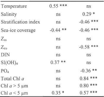
Table 1: Distribution of major taxonomically significant pigments in algal classes using SCOR abbreviations (Jeffrey and Vesk 1997) ... 28 Table 2: Spearman correlation coefficients between phytoplankton abundance and environmental and biological factors at ail stations and depths. Because of their low abundance, excluding picocyanobacteria and microphytoplankton from these correlations do not affect the significance of the correlation coefficients. *p < 0.05; ** p < 0.01; *** p < 0.001; ns: not significant. ... 36
Table 3: Abundance of photosynthetic picoeukaryotes and of the picocyanobacteria
Synechococcus sp. in the Arctic Ocean and adjacent seas. Sea surface
temperature and salinity are shown. a: picoeukaryote <5 !lm; b: early fall (September-October); c: summer (July-September); d: late summer
LISTE DES FIGURES
Page 1. INTRODUCTION GÉNÉRALE
Figure 1: Chaîne trophique classique (herbivore) versus la boucle microbienne (Tirée de Steele 1974) ... 4 Figure 2: Représentation schématique de l'installation des écosystèmes pélagiques
(Adaptée de Legendre et Rassoulzadegan 1995) ... 6
II. PHYTOPLANKTON DISTRIBUTION ALONG A 3500 KM TRANSECT IN CANADIAN ARCTIC WATERS IN LATE SUMMER: STRONG DOMINANCE OF PICOEUKARYOTES
Figure 1: Location of the sampling stations in the Canadian High Arctic visited from 16 August to l3 September 2005. Open (0) and solid (e) dots indicate open water and ice-covered conditions, respectively. Three oceanographic provinces were identified: the Beaufort Sea (Stns 10, Il, 12, 204, CA04, CA05, CA08 and CA18), the Northwest Passage (Stns 3, 4, p, 6 and 7) and the northem Baffin Bay (Stns BA01, BA02, BA03, BA04 and 2) ... 23 Figure 2: Variations of the (A) water depth, (B) sea-lce coverage, (C) depths of the
euphotic zone (Zeu) and the surface mixed layer (Zm), and (D) vertical stratification index (the difference in sigma-t between 80 and 5 m) along a transect across the Canadian High Arctic. AlI stations are plotted against longitude, except for stations in northem Baffin Bay, which are plotted against
XlI
latitude. In (C), Zeu at Stns p and 204 were estimated from the values measured at the two nearest stations ... 31
Figure 3: Variations of(A) water temperature, (B) salinity, (C) dissolved inorganic nitrogen (DIN = N03 + N02 + NH4) concentration, and (D) silicic acid (Si(OH)4) concentration at three sampled depths in the euphotic zone along a transect across the Canadian High Arctic ... 32
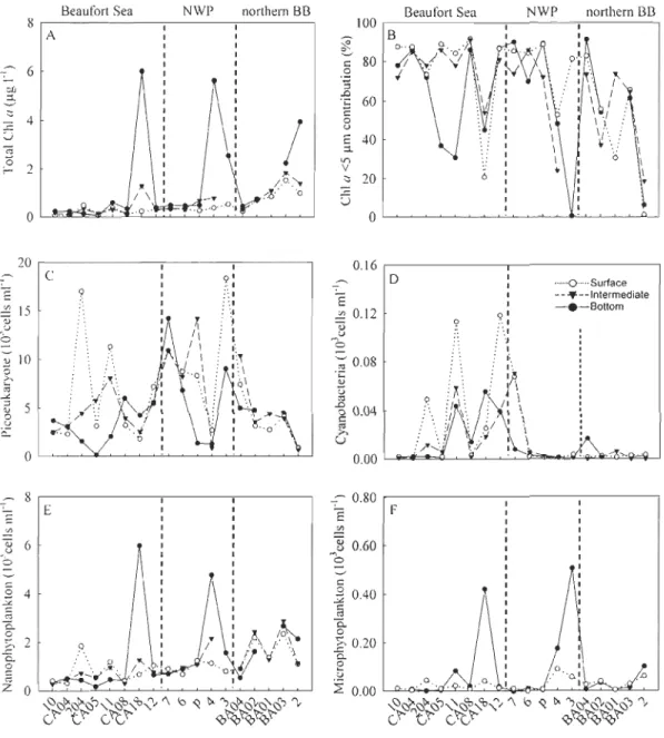
Figure 4: Variations of (A) total chlorophyll a (ChI a) biomass, (B) percent contribution of small algae «5 J.Lm) to total ChI a biomass, (C) picoeukaryote abundance, (D)
cyanobacteria abundance, (E) nanophytoplankton abundance, and (F)
microphytoplankton abundance at three sampled depths in the euphotic zone. In (F), the intermediate depth was not sampled ... 34
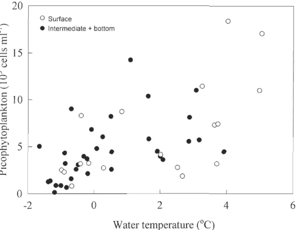
Figure 5: Relationship between picophytoplankton abundance and water temperature (X2
=
2.2x,+
3.4, r2=
0.35). Black dots represent samples collected in the intermediate and bottom layers of the euphotic zone whereas the open dots represent samples collected in the surface layer ... 35Figure 6: Relationship between nanophytoplankton abundance estimated by flow cytometry (FCM) and light microscopy (LM) (y
=
0.7x+
85.8, r2=
0.91, p < 0.0001). The outlier identified by an open circle was excluded from the regression. The dashed line represents a slope of 1 ... 39 Figure 7: Variations of the relative abundance ofthree different plankton groups (diatoms,dinoflagellates, flagellates) in (A) the surface layer, and (B) at the bottom layer of the euphotic zone along a transect across the Canadian High Arctic ... .40
Figure 8: Percent contribution of specific accessory pigments (SAP) to total pigments for four groups of biomarkers collected in the surface waters. SAP for the pico type
group are: ChI h, MgDVP, Mmnal, Neo, Lut, Viola, Pras, Uriolide and Zea. SAP
for the nana type group are: Fuco, ChI C2+Cl, ChI C3, Hex-fuco, But-fuco, Allo, Diato and Diadino. SAP for the degradation products group are: Chlde a, Phe and
Pyro-Pheo. SAP for the other group are: Per and p,p-carot. See Table 1 for
pigment abbreviations ... .44
Figure 9: Relationships between percent contribution of picophytoplankton to total phytoplankton abundance (pico-
+
nano-+
microphytoplankton) and percentcontribution ofpicophytoplankton to total ChI a biomass for (A) Beaufort Sea, (B)
Northwest Passage (NWP) , and (C) northern Baffin Bay (BB). The error bars represent the standard error for the three sampled depths in the euphotic zone (i.e.
surface, interrnediate and bottom) ... 45 Figure 10: Relationship between maximum eukaryote picophytoplankton abundance and
surface water temperature from six studies conducted in circumarctic regions in
INTRODUCTION GÉNÉRALE
Le terme plancton a été défini scientifiquement pour la première fois par Hensen (1887) permettant de caractériser l'ensemble des organismes vivants, animaux et végétaux,
qui flottent dans les eaux. Bien que certains organismes planctoniques puissent atteindre
des tailles importantes, comme les méduses, la très grande majorité du plancton est tellement minuscule que l'utilisation d'un microscope devient essentielle pour en faire
l'observation. Ces organismes planctoniques peuvent être caractérisés en se basant sur leur
rôle fonctionnel dans l'écosystème, ou encore selon des critères génétiques, taxinomiques
(Stockner et Antia 1986) ou de taille (Sieburth et al. 1978).
Dans sa conception la plus élémentaire, la classification des orgamsmes planctoniques est constituée par le zooplancton (organismes animaux pluricellulaires), le phytoplancton (incluant les cellules végétales eucaryotes et procaryotes) et le bactérioplancton (cellules procaryotes hétérotrophes). Le critère de taille du plancton permet de distinguer des compartiments écologiques auxquels correspondent des classes de taille relativement bien définies. Dans ce mémoire nous nous intéresserons surtout au
microphytoplancton (20-200 )lm), au nanophytoplancton (2-20 )lm) et au
Réseaux trophiques pélagiques
Comme dans tous les écosystèmes terrestres et aquatiques, les végétaux
chlorophylliens représentent le premier maillon de la chaîne trophique assurant la fixation du carbone. En se référant à la structure de taille des organismes phytoplanctoniques, notamment la partition entre les petites «5 )lm) et les grandes (>5 )lm) cellules, quatre types d'écosystèmes pélagiques marins ont été décrits. Il est admis que lorsque les
concentrations d'azote sont faibles, les petites cellules sont plus efficaces dans l'absorption de l'ammonium comparé aux grosses cellules. Seulement deux des quatre types
d'écosystèmes pélagiques marins seront décrits dans le présent mémoire puisqu'ils représentent les situations extrêmes contrairement aux deux autres types intermédiaires.
La chaîne trophique classique dominée par le réseau herbivore représente le système le plus simple (Fig. 1). Il repose essentiellement sur l'assimilation des éléments nutritifs, principalement le nitrate, par de grandes cellules phytoplanctoniques lesquelles seront
broutées par le zooplancton herbivore (e.g., les copépodes) qui sera à son tour consommé par les carnivores de premier ordre (Steele 1974). La forte concentration en nitrates dans le milieu va donc favoriser le développement des grosses cellules phytoplanctoniques au
détriment des plus petites. Ce système est particulièrement efficace dans l'exportation du
carbone en profondeur. Cette chaîne alimentaire simple est toutefois insuffisante pour comprendre l'ensemble des processus existant au sein du système planctonique.
3
Pomeroy (1974) et Azam et al. (1983) ont démontré que les cellules
picophytoplanctoniques autotrophes et hétérotrophes constituent une importante source d'énergie au sein de ce que nous appelons maintenant la boucle microbienne (Fig. 1). Dans ce système, les apports en éléments azotés sont quasi nuls alors que la matière organique dissoute excrétée par le phytoplancton et générée par l'activité du zooplancton (e.g., bris de
cellules, excrétion, pelotes fécales) est consommée efficacement par les bactéries hétérotrophes. Ces mêmes bactéries entrent alors en compétition directe avec le phytoplancton de petite taille pour l'ammonium. Le système repose sur l'excrétion d'ammonium et représente ainsi un circuit en boucle fermé. Ce type d'écosystème se
caractérise par une relative inefficacité de l'exportation du carbone. La faible sédimentation et le recyclage rapide de la matière sédimentaire font en sorte que le transfert d'énergie vers
le réseau trophique supérieur est faible.
L'instauration d'un réseau trophique pélagique dépend des conditions du milieu
auxquelles est soumis le phytoplancton. Les algues phytoplanctoniques ont développé des
adaptations morphologiques leur permettant de se maintenir dans la couche de surface où la photosynthèse est possible, résultant d'une adaptation acquise au fil du temps. Par contre,
les organismes phytoplanctoniques subissent les variations de leur environnement et
doivent donc s'y adapter de manière à pouvoir se développer. La lumière incidente et la turbulence constituent les principaux facteurs de contrôle de la production primaire dans les
Nutriments Matière organiqu dissoute
\
,
'~~
l
'
"-
...J--..,~
~,
meso- ' \ zoo- -plancton ' n Il' 1 age es,T
ciliés" Boucle microbienne
Niveaux trophiques supérieurs
CNllnè trophiquE' classique
Voies de mineralisation
Voies de la matière organique dissoute
Figure 1 : Chaîne trophique classique (herbivore) versus la boucle microbienne (Tirée de
5
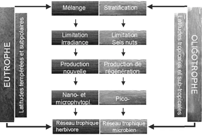
que les caractéristiques hydrodynamiques de la colonne d'eau influençaient les apports en éléments nutritifs et la lumière incidente disponible, le type de production phytoplanctonique qu'elle soit nouvelle ou régénérée ainsi que le type de micro-organismes présents (Fig. 2). Dans un milieu bien mélangé, la lumière incidente devient la variable environnementale limitante et la production nouvelle est alors dominée par le nanophytoplancton et le microphytoplancton de telle sorte que s'installe un réseau trophique herbivore. Ce type de réseau trophique est principalement retrouvé dans les écosystèmes côtiers et eutrophes. En contrepartie dans un milieu stratifié, ce sont les éléments nutritifs qui deviennent limitants et la production régénérée est alors dominée par le picophytoplancton (cellules flagellées autotrophes, bactéries hétérotrophes et cyanobactéries) de telle sorte qu'un réseau trophique microbien prend place. Ce type de réseau est surtout observé dans les écosystèmes océaniques et oligotrophes, pauvres en éléments nutritifs.
Répartition du microphytoplancton et du nanophytoplancton
Le microphytoplancton (20-200 ~m) et le nanophytoplancton (2-20 ~m) se composent de diatomées, de dinoflagellés et de flagellés. Les diatomées (Bacillariophyta) ont longtemps été reconnues comme étant le principal groupe du phytoplancton marin. On estime annuellement la production primaire marine à 60 Gt de carbone, dont une
contribution de quelque 25 Gt de carbone qui serait imputable aux diatomées (Nelson et al. 1995). Les diatomées sont divisées en deux groupes: les Centrales qui présentent une symétrie radiale et une forme généralement circulaire et les Pennales qui ont une symétrie
"-~ _ _ • V~:;J> ',;; L ''JO t ~" •
Mélange
--"
Limitation
Irradiance
~- ,.. ,.,,,..,.,,Production
nouvelle
',~_. '
Nanc;:.
'
et
~-. ,
micro h to
1.
'
Reséau trophique
herbivore
Figure 2: Représentation schématique de l'installation des écosystèmes pélagiques
7
bilatérale et une forme allongée linéaire-lancéolée. Il est à noter que l'usage de ces termes n'est aucunement valide sur le plan nomenc1atural. Les diatomées centrales sont prépondérantes dans les écosystèmes marins côtiers et océaniques avec, par exemple, une abondance marquée du genre Skeletonema Greville lors des floraisons de fin d'hiver ou
encore des genres Chaetoceros Ehrenberg et Thalassiosira Cleve rencontrés pendant les floraisons printanières. Quant aux dinoflagellés, ce sont des organismes autotrophes et hétérotrophes unicellulaires qui se retrouvent aussi bien parmi le microphytoplancton que le nanophytoplancton. Les dinoflagellés tirent avantage de leur capacité à se mouvoir puisqu'ils peuvent se déplacer dans la colonne d'eau lorsque, par exemple, la turbulence des eaux est faible.
La première étude sur la composition du phytoplancton des mers arctiques remonte à Cleve (1896) qui a analysé une cinquantaine d'échantillons de la baie de Baffin et du détroit de Davis. Quelques années plus tard, Gran (1904) a recensé les mêmes espèces retrouvées par Cleve (1896), en y ajoutant deux nouvelles espèces en provenance de la mer du Groenland. Il a de plus distingué les espèces issues des glaces de mer telles que
Nitzschia frigida Grunow et Melosira hyperborea Grunow (=Melosira arctica Dickie) de
celles de la colonne d'eau (Chaetoceros spp. et Thalassiosira spp.). Selon Heimdal (1989), aucune recherche sur la dynamique du phytoplancton en relation avec son environnement arctique n'a été faite avant les années 1930. Gmntved et Seidenfaden (1938) ont été les premiers à présenter les données sur la répartition spatiale du phytoplancton dans la région de la polynie des Eaux du Nord (NOW), à l'ouest du Groenland. C'est pour ainsi dire la
première étude exhaustive démontrant que la polynie NOW est parmi les régions maritimes les plus productives au nord du cercle arctique. D'autres études ont suivi fournissant des comptes-rendus sur la répartition du phytoplancton dans d'autres régions de l'Arctique telles que la côte ouest de Svalbard (RamsfjellI954), la baie d'Hudson (Bursa 1961), Pond Inlet (Cross 1982), et en bordure de la banquise en mer du Groenland (Spies 1987). Des
études plus récentes ont permis la reconnaissance d'espèces dominantes en régions
arctiques (Booth et Homer 1997, Booth et Smith 1997, Jensen et Hansen 2000, von Quillfeldt 2000, Booth et al. 2002, Lovejoy et al. 2002, Rat'kova et Wassmann 2002), contribuant ainsi à améliorer nos connaissances sur la répartition du phytoplancton dans l'Arctique et, plus particulièrement, celle des cellules de taille plus grande que 2 /-lm.
Le microphytoplancton et le nanophytoplancton sont généralement associés aux
latitudes nord et sud des eaux tempérées ainsi que dans les régions de résurgence
équatoriale (Tarran et al. 2006). En régions polaires, la présence du microphytoplancton et
du nanophytoplancton dépend surtout de la fonte des glaces de mer annuelles et elle est
restreinte essentiellement à certaines périodes de l'année (Gosselin et al. 1997, Lovejoy et al. 2002, Wassmann et al. 2006). L'étendue et la couverture des glaces de mer de première année contrôlent la disponibilité de la lumière incidente, limitent la formation d'une
stratification de la colonne d'eau et empêchent un mélange vertical normalement induit par
l'action du vent (e.g. Mei et al. 2003). La compilation de résultats échelonnés sur une dizaine d'années dans le détroit de Barrow et le Passage du nord-ouest a permis à Michel et al. (2006) d'établir que la floraison phytoplanctonique survenait au cours du mois de juillet
9
au moment même de la fonte des glaces de mer annuelles. Pour sa part, Hsiao (1996) a établi pour la mer de Beaufort que les diatomées et les flagellés représentaient les organismes phytoplanctoniques contribuant le plus à la production primaire pendant la
saison estivale libre de glace, c'est-à-dire en juillet et en août. Par contre, dans les polynies des Eaux du Nord (NOW) et du Nord-Est (NEW), de part et d'autre du Groenland, les diatomées ont fait leur apparition aussi hâtivement qu'en mars, permettant ainsi de rallonger la période de production (Mei et al. 2002, Tremblay et al. 2006).
Répartition du picophytoplancton
Le microphytoplancton et le nanophytoplancton peuvent être facilement filtrés sur différents types de membranes pour ensuite y être identifiés et dénombrés par la microscopie optique. Par contre, les cellules picophytoplanctoniques, étant de plus petites tailles, deviennent pratiquement impossibles à y être observées par la microscopie conventionnelle. Les avancés technologiques récentes ont toutefois permis non seulement de reconnaître mais aussi d'identifier des cellules de plus en plus petites (Stockner et Antia 1986). Les études en cytométrie de flux ont ainsi permis de démontrer que le picophytoplancton autotrophe est composé de deux principaux genres de cyanobactéries,
Prochlorococcus Chisholm, Frankel, Goericke, OIson, Palenik, Waterbury, West-Johnsrud
et Zettler (Johnson et Sieburth 1979) et Synechococcus Nageli (Waterbury et al. 1979),
ainsi que de très petites cellules eucaryotes (Campbell et al. 1994). La principale distinction
entre ces deux genres de cyanobactéries repose essentiellement sur la forte fluorescence orange émise par le pigment de la phycoérythrine présente chez les Synechococcus.
L'utilisation de la biologie moléculaire a aussi permis d'améliorer nos connaissances des
caractéristiques physiologiques et des mécanismes d'adaptation des cyanobactéries. Par
contre, nous commençons à peine à mettre en lumière le picophytoplancton eucaryote et
d'en identifier les principaux groupes (Worden 2006).
Depuis la découverte des cyanobactéries Prochlorococcus et Synechococcus, de
nombreuses études ont porté sur le rôle exercé par le picophytoplancton dans le
fonctionnement des écosystèmes côtiers pélagiques (e.g., Li 1994, Worden et al. 2004,
Maixandeau et al. 2005). Le picophytoplancton se retrouve habituellement dans les régions
océaniques oligotrophes avec des abondances relativement constantes et élevées variant
entre 107 et 109 cellules rI (Stockner et Antia 1986). Le picophytoplancton est dominant
non seulement en terme de production primaire en dehors des périodes de floraisons
habituelles de diatomées ou de dinoflagellés (Bell et Kalff 200 1, Durand et al. 2001), mais
il représente aussi une contribution importante à la biomasse phytoplanctonique (Partensky
et al. 1999, Sherr et al. 2003). Cette prépondérance du picophytoplancton s'explique, entre
autres, par la très petite taille des cellules associée à une faible vitesse de chute (loi de
Stokes), leur assurant ainsi un avantage certain sur l'absorption d'éléments nutritifs en
faible concentration ambiante (Raven 1998).
Le genre Prochlorococcus fait partie des cyanobactéries marines photosynthétiques
dont la taille des cellules est d'environ 0,6 !lm. Ce genre est surtout numériquement
Il
et 40oS, quoique Buck et al. (1996) ont observé la présence de Prochlorococcus jusqu'à la latitude 61°N. Selon Partensky et al. (1999), il serait l'organisme photo synthétique le plus abondant en terme de nombre d'individus dans les océans. Dans les eaux oligotrophes de l'Atlantique et du Pacifique, les cellules de Prochlorococcus sont présentes jusqu'à des profondeurs largement supérieures à celles de la zone euphotique (Partensky et al. 1999).
Dans l'océan Atlantique, Prochlorococcus est particulièrement abondant dans les gyres tropicales où les éléments nutritifs sont presque absents alors que la température de l'eau se situe autour de 24°C, se rapprochant ainsi des conditions optimales pour leur croissance (Partensky et al. 1999). Agusti (2004) a d'ailleurs démontré que la croissance des cellules de Prochlorococcus était négativement corrélée avec la concentration en nitrate des eaux de surface (Pearson r = -0,77, P < 0,05). De plus, Vaulot et al. (1995) et DuRand et al. (2001) ont calculé que les cellules de Prochlorococcus contribueraient entre 21 % et 43% de la biomasse phytoplanctonique et entre 13% et 48% de la production primaire dans les océans oligotrophes.
Pour sa part, le genre Synechococcus dont la taille des cellules varie entre 0,8 et 1,5 !lm regroupe des cyanobactéries planctoniques photosynthétiques abondantes en milieu marin, et plus particulièrement en milieu côtier (Stockner 1988, Partensky et al. 1999).
Plusieurs espèces dulcicoles de Synechococcus ont aussi été décrites récemment, certaines occupant même des habitats extrêmes tels que des sources géothermales, des eaux riches en soufre ou encore pauvres en oxygène, et même des milieux appauvris en éléments nutritifs (Stockner et al. 2000). Synechococcus est principalement retrouvé dans la plupart des
océans et des mers oligotrophes-mésotrophes des Tropiques jusqu'aux régions polaires (Shapiro et Haugen 1988). D'ailleurs Gradinger et Lenz (1989) et Not et al. (2005) ont démontré la présence de Synechococcus dans les eaux arctiques, plus particulièrement dans les masses d'eau influencées par les courants en provenance de l'Atlantique. Tout récemment, Waleron et al. (2007) ont mis en évidence l'importance des apports allochtones de Synechococcus dans l'Arctique de l'ouest par l'intermédiaire des rivières Mackenzie en mer de Beaufort et Horton en baie de Franklin. L'importance des cellules de Synechococcus
sur le transfert d'énergie vers les niveaux trophiques supérieurs dans les eaux arctiques n'a pas autant d'impact que dans le cas des cellules pico eucaryotes (Gradinger et Lenz 1995), ces dernières étant plus importantes à la fois en terme de biomasse et d'abondance dans les
eaux arctiques (Smith et al. 1985).
Quant aux cellules pico eucaryotes, elles présentent une très grande diversité et elles dominent numériquement la communauté picophytoplanctonique dans les gyres oligotrophes de l'Atlantique et du Pacifique (Tarran et al. 2006). Certaines études ont même démontré que les cellules picoeucaryotes, incluant les chlorophytes et les prasinophytes dont principalement Micromonas pusilla (Butcher) Manton et Parke, peuvent aussi être prépondérantes en milieu côtier (Not et al. 2004, Romari et Vau lot 2004, Worden 2006). En milieu océanique, les cellules picoeucaryotes sont surtout observées en profondeur à la base de la zone euphotique correspondant au 0,5% de la lumière incidente de surface (Glover et al. 1986). L'abondance du picophytoplancton suit également un cycle saisonnier semblable à celui des cellules phytoplanctoniques de plus grande taille, avec un
13
maximum généralement observé en été (Stockner et Antia 1986). Les cellules picoeucaryotes sont responsables d'une grande fraction de la biomasse de carbone en comparaison des cyanobactéries (Li 1994, Tarran et al. 2006). Par exemple, dans le Pacifique nord et le sud de la mer de Béring, Liu et al. (2002) ont démontré qu'à la fin de la saison estivale, les cellules eucaryotes étaient beaucoup plus importantes en terme de biomasse pour le compartiment pico-autotrophe.
Les études sur la répartition géographique du phytoplancton dans les régions arctiques ont longtemps mis l'emphase sur les cellules microphytoplanctoniques et nanophytoplanctoniques (Murphy et Haugen 1985, von Quillfeldt 1997), favorisant ainsi la conception d'un réseau trophique classique ou herbivore. Au cours de la dernière décennie,
plusieurs travaux ont démontré que les régions arctiques favorisaient la prépondérance de cellules picoeucaryotes (Booth et Smith 1997, Booth et Homer 1997, Not et al. 2005, Lovejoy et al. 2006). En mer de Barents, Not et al. (2005) ont mesuré des abondances de cellules picoeucaryotes dans les eaux d'origine Arctique variant entre 2600 et 10 200 cellules mr'. Les cellules picoeucaryotes, plus particulièrement la classe des Prasinophyceae, sont aussi très présentes dans les régions arctiques représentant entre 40%
et 80% de la biomasse chlorophylienne annuelle, à l'exception toutefois du mois de juillet (Lovejoy et al. 2007). Selon les études de Not et al. (2005) et de Lovejoy et al. (2007),
Micromonas pusilla est l'organisme eucaryote dominant dans les eaux arctiques. Cette
prasinophyte représente un écotype distinct pour les régions arctiques avec une étroite niche thermale (Lovejoy et al. 2007). Ces dernières découvertes mettent ainsi en évidence
l'importance du réseau pélagique microbien dans l'Arctique (Lovejoy et al. 2007). Il en
ressort que l'observation des spectres de taille dans l'environnement peut donner une très
bonne indication de la structure trophique du domaine pélagique d'une région aussi vaste
que celle représentée, par exemple, par l'Arctique.
Région sous étude
La région étudiée se situe en plein cœur du Haut Arctique canadien, s'étalant depuis
la baie de Baffin jusqu'en mer de Beaufort en passant par le Passage du nord-ouest,
c'est-à-dire représentant une distance d'à peu près 3500 km. Cette vaste région est sous l'influence
d'entrée d'eaux du Pacifique à l'ouest et de l'Atlantique à l'est. Par conséquent, ces deux
types de masses d'eau ont des propriétés physico-chimiques différentes; l'eau provenant du
Pacifique est moins salée et riche en éléments nutritifs et l'eau originant de l'Atlantique est
plus salée et moins riche en éléments nutritifs (Jones et al. 1998, Tremblay et al. 2002). Les
changements apportés par le réchauffement planétaire (ACIA 2005) entraînent déjà (1) une
réduction de la couverture des glaces annuelles influençant la pénétration de la lumière et la
stratification des eaux ouvertes (Smetacek et Nicol 2005) et (2) des changements dans la
circulation océanique (Kliem et Greenberg 2003) qui résultent en une augmentation de la
température de l'eau atlantique entrant dans l'océan Arctique (Polyakov et al. 2004). Il est
très certainement envisageable de prévoir de nouvelles perturbations du milieu qui
influenceront alors la répartition du micro-, du nano- et du picophytoplancton dans le Haut
Arctique canadien, modifiant ainsi le réseau trophique pélagique arctique et les flux
15
spatiale actuelle des différents groupes phytoplanctoniques nous permettra de mieUX prévoir la réponse du phytoplancton arctique à une réduction de la couverture de glace, à un accroissement de la stratification de la colonne d'eau et à une augmentation de la température des eaux de surface.
Objectifs de la recherche
La présente étude vise à évaluer la répartition spatiale et l'abondance du pico-, du nano- et du microphytoplancton du Haut Arctique canadien depuis la baie de Baffin jusqu'en mer de Beaufort en passant par le Passage du nord-ouest à la fin de la période estivale. Les deux objectifs spécifiques à cette étude sont: 1) décrire la répartition spatiale du micro-, du nano- et du picophytoplancton dans les trois régions océanographiques du Haut Arctique canadien et 2) évaluer les variables environnementales gouvernant la répartition du phytoplancton.
II. PHYTOPLANKTON DISTRIBUTION ALONG A 3500 KM TRANSECT IN CANADIAN ARCTIC WATERS IN LATE SUMMER: STRONG DOMINANCE OF
17
ABSTRACT
A number of recent studies showed that photosynthetic picoeukaryotes are an active and often dominant component of the Arctic algal assemblage. In order to extend these
observations, samples from the euphotic zone were collected at 18 stations along a transect from the northern Baffin Bay to the Beaufort Sea through the Northwest Passage in late summer 2005. Picophytoplankton «2 /lm) and nanophytoplankton cells (2-20 /lm) were enumerated using flow cytometry and phytoplankton cells >2 /lm were identified and counted by light microscopy. In addition, algal pigment composition was assessed by reverse-phase high-performance liquid chromatography to determine to which algal groups belong the smallest cells. The spatial phytoplankton distribution was heterogeneous along the transect. Maximum picophytoplankton abundance was observed in the Beaufort Sea/Northwest Passage region, whereas nanophytoplankton abundance tended to increase toward the eastern Canadian Arctic. Picophytoplankton abundance and total chlorophyll a biomass reached values as high as 18,400 cells mrl and 6 /lg rI. Picophytoplankton abundance and chlorophyll a <5 /lm made up >70 % of total phytoplankton abundance and biomass in 70 % of the collected samples. Throughout the transect, picophytoplankton cells were largely dominated by eukaryotes (presumably the Prasinophyceae Micromonas). Maximum abundances of picocyanobacteria (120 cells mrl) were observed in brackish waters of the Beaufort Sea. These results confirm that picophytoplankton can dominate not only in warm oligotrophic waters, but also in a perennially cold ocean in late summer.
INTRODUCTION
The size distribution of phytoplankton assemblages is a major biological factor that govems the functioning of the pelagic food web and, consequently, affects the rate of carbon export from the open ocean surface waters to the deep layers (Legendre & LeFèvre
1991). Large, rapidly sinking phytoplankton cells such as diatoms, are believed to control the carbon flux from the upper ocean layers (Michaels & Silver 1988), and to efficiently
transfer energy to the upper trophic levels (Cushing 1989). Large diatoms are at the base of herbivorous food webs, supporting renewable marine resources such as herbivorous zooplankton and fish (Cushing 1989). In contrast, small phototrophic picoplankton (cells
from 0.2 to 2 )lm; Sieburth et al. 1978) are believed to be recycled within the microbial loop (Azam et al. 1983) contributing less efficiently to the transfer of energy and matter to the upper trophic levels. Picophytoplankton cells are also considered to contribute less to the sinking material because of their low sinking fluxes (Michaels & Silver 1988).
However, Richardson & Jackson (2007) have shown that the relative contribution of
picophytoplankton to carbon export can be proportional to their total net primary production because of their incorporation into aggregates that can settle or be grazed by mesozooplankton. Considering the finding of Richardson & Jackson (2007), the
conventional VleW that picophytoplankton contribute little to carbon export should be revisited.
19
Large phytoplankton cells, inc1uding diatoms, pryrnnesiophytes and dinoflagellates,
produce seasonal blooms under specific hydrographic conditions (Mei et al. 2002). For instance, the production of large phytoplankton is governed by variations in the vertical stability of the water colurnn, through the effects on nutrient replenishment and the residence time of algal cells in the euphotic zone (Tremblay et al. 1997). In addition, the duration of the production period is sensitive to the seasonal melt dynamics of sea ice (Fortier et al. 2002). In northern Baffin Bay, intense diatom bloom characterized by cells >5 !lm, begins as early as the end of April when the North Water polynya opens up (Mei et al. 2003). In the Canadian Archipelago, particularly in Barrow Strait, the phytoplankton bloom typically develops in July and August, corresponding to the timing of the ice break-up for this region (Michel et al. 2006). In the Chukchi and Beaufort seas, high chlorophyll concentrations are observed in regions along the ice edge, and are associated with an overwhelming predominance of diatoms and haptophytes (Hill et al. 2005). In the Barents Sea, large-celled phytoplankton dominate during blooms occurring in the marginal ice zone (Wassmann et al. 2006) and are of particular importance to the production of organic matter and vertical export of carbon (Sakshaug & Skjoldal 1989).
Several studies have shown that small phytoplankton cells «5 !lm) can also have an important role in carbon fixation in the Arctic Ocean and adjacent seas (Legendre et al. 1993, Pesant et al. 1996, Gosselin et al. 1997). Picophytoplankton contribute for most of the production and biomass in warm and nutrient-poor waters (Agawin et al. 2000). Recent studies have shown that picophytoplankton are often well-represented in terms of abundances in co Id Arctic seawaters. Indeed, eukaryotic cells <2 !lm often dominate the
phytoplankton assemblage reaching abundances in the order of 1000-10,000 cells mr' in
the central Arctic Ocean (Booth & Homer 1997) in summer, of 2600-10,200 cells mr' in
Arctic waters of the Barents Sea (Not et al. 2005) in late summer, and up to
28,000 cells mr' during the initial spring bloom and between 1000 to 10,000 cells mr'
during the rest of the growth season in the central Arctic Ocean (Sherr et al. 2003). Within
these small eukaryotic ceIls, Not et al. (2005) showed that the prasinophyte Micromonas
pusilla (Butcher) Manton et Parke made up 32 % of total picoeukaryotic cells at stations
located in truly Arctic waters, but only 9 % at stations influenced predominantly by
Atlantic waters. In addition, Lovejoy et al. (2007) recently demonstrated that
picoprasinophytes are spatially and temporally prevalent throughout the Arctic region
where M pusilla is the most abundant picoeukaryote representing a single high-latitude
ecotype.
In contrast to photosynthetic picoeukaryotes, picocyanobacteria are generally poorly
represented in the Arctic seas (Murphy & Haugen 1985, Booth & Homer 1997, Mostajir et
al. 200 1, Sherr et al. 2003), in strong contrast with their high abundance in Arctic lakes and
ri vers (Vincent 2000). In the Southem Ocean, picocyanobacteria abundance decreases with
increasing latitude, i.e. with decreasing temperature (Marchant et al. 1987). In the Arctic
Ocean and adjacent seas, the two main sources ofpicocyanobacteria are Atlantic waters and
freshwater river input. Not et al. (2005) have shown high abundances of the
picocyanobacteria Synechococcus Nageli in the Atlantic influenced-waters of the Barents
Sea, which are characterized by high surface water temperature. This corroborates earlier
21
influenced-waters into the Arctic seas (Murphy & Haugen 1985, Gradinger & Lenz 1989).
In the Laptev Sea, Moreira-Turcq & Martin (1998) observed maximum picocyanobacteria
concentration in brackish water near the Lena River delta, but their absence at salinity >20. More recently, Waleron et al. (2007) suggested from 16S rRNA gene clone libraries that picocyanobacteria present in the Canadian Beaufort Sea originated from the Mackenzie River and other nearby inflows.
The cell size of phytoplankton taxa present in the ocean is, in part, determined by
environmental and physiological factors, as demonstrated by Parsons & Takahashi (1973).
Given the transition towards a new, warmer state (Polyakov et al. 2005), it is expected that
the relative abundance of pico- versus larger phytoplankton will change in Arctic regions. The objectives of the present study were to (1) determine the distribution of pico-,
nano-and microphytoplankton in three contrasted oceanographic provinces of the Canadian High
Arctic in late summer and (2) assess the influence of environmental factors on the
phytoplankton abundance and biomass of each size fraction. It was hypothesized that
picocyanobacteria would be present in Atlantic influenced-waters and nearby river inflows. The photosynthetic picoeukaryote abundance was expected to be higher in warm stratified
waters than in cold deeply mixed waters. Finally, in agreement with comprehensive reviews
of the available literature (Agawin et al. 2000, Bell & Kalff 2001), the large phytoplankton
MATERIALS AND METHODS
Study sites and sampling
This study was conducted in the Canadian High Arctic from 16 August to 13 September 2005, hereafter referred to as late summer, over a 3500 km longitudinal transect,
as part of the ArcticNet research pro gram on board the CCGS Amundsen. A total of 18
stations were visited consisting of five stations in northem Baffin Bay (northem BB: Stns BA01 to BA04 and 2), five stations in the Northwest Passage (NWP: Stns 3, 4, p, 6 and 7)
and eight stations in the Beaufort Sea (Stns 10 to 12,204, CA04, CA05, CA08 and CA18)
(Fig. 1). Water samples were collected at three depths (50, 15 % of surface irradiance and
at the maximum chlorophyll a (ChI a) fluorescence depth) with a rosette sampler equipped
with 121 Niskin-type bottles (OceanTest Equipment), an in situ fluorometer (SeaPoint) and
a high precision CTD (conductivity-temperature-depth instrument) probe (Sea-Bird 911 +). Since the depth of the maximum ChI a fluorescence was generally 10cated between 0.2 and
5 % surface irradiance, the three sampling depths are hereafter referred to as surface, intermediary and bottom layers of the euphotic zone, respectively.
Physical and chemical measurements
Incident photosynthetically available radiation (Ed(PAR); 400-700 nm) was measured continuously during the expedition with a LICOR sensor (LI-190SA). Downwelling PAR underwater profiles were measured using a light sensor (Biospherical QCP-2300) mounted on the CTD rosette, except at Stns 3, 7, Il where a PNF-300
78
76
...-...z
o ----~74
:::J ... :.;:. co ...J72
70
10•
140
CA04•
---""-~==-
.;J
o:
.
x-120
.
....
100
Longitude ("W)23
m
80
Fig. l. Location of the sampling stations in the Canadian High Arctic visited from 16 August to 13 September 2005. Open (0)
and solid (e) dots indicate open water and ice-covered conditions, respectively. Three oceanographie provinces were
identificd: the Beaufort Sea (Stns 10, Il, 12,204, CA04, CA05, CA08 and CA18), the Northwest Passage (Stns 3,4,
p, 6 and 7) and the northem Baffin Bay (Stns BAOl, BA02, BA03, BA04 and 2)
100
250
1000
radiometer (Biospherical Instruments) was used. The vertical attenuation coefficient for downward PAR (~(PAR)) in the euphotic zone was determined by linear regression of the natural logarithm of Ed(P AR) versus depth. The euphotic depth (Zeu) was defined as the depth receiving 1 % of the surface irradiance. The surface mixed layer depth (Zm) was determined using a split-and-merge method (Thomson & Fine 2003). Zm was also determined from the density (sigma-t) differences of 0.03 kg m-3. There was a strong linear relationship between the surface mixed layer depths determined from the 0.03 kg m-3
criterion (y) and the Thomson & Fine method (x) (y
=
0.98x - 0.10; 95 % CI from 0.66 tol.20, r2 = 0.91, P < 0.0001). An index of the vertical stratification of the water column was
estimated as the difference in the sigma-t between 80 and 5 m. The presence of ice was
estimated visual!y at each station. Samples for nitrate (N03), nitrite (N02), silicic acid
(Si(OH)4) and phosphate (P04) determination were processed immediately after sampling
on board the ship using a Bran-Luebbe III autoanalyzer (Grasshoff et al. 1999).
Biological measurements
Flow cytometry (FCM) analysis. Duplicate water samples (5 ml) for the determination of pico- and nanophytoplankton abundance were fixed with 0.1 % final concentration
glutaraldehyde (Marie et al. 2005), stored in liquid nitrogen on board the ship and kept
frozen at -80DC for a week before analysis. Samples were analyzed using an Epics Altra
flow cytometer (Beckman-Coulter) equipped with a 488 nrn laser (15 mW output). Forward angle light scatter (FALS), right angle light scatter (RALS), orange fluorescence from phycoerythrin (575 ± 20 nm) and red fluorescence from chlorophyll (675 ± 10 nm) were measured. Prior to analysis, samples were pre-screened on a 40 f.Lm Nylon cel! strainer.
25
One !lm microspheres (Fluoresbrite plain YG, Polysciences) were added to each sample as an internaI Standard. Pico- «2 !lm) and nanophytoplankton (2-20 !lm) were discriminated
based on forward scatter calibration with polystyrene microspheres of known size. The
average coefficients of variation on the duplicate samples were 5.7 % and 12.5 % for
pico-and nanophytoplankton abundances, respectively. The average of the two duplicates is presented thereafter.
Light microscopy (LM) analysis. Samples for the identification and enumeration of
eukaryotic cells >2 !lm were collected at two depths (the surface and at the bottom layers of
the euphotic zone). They were preserved in acidic Lugol's solution (Parsons et al. 1984)
and stored in the dark at
4°e
until analysis. Samples were identified to the lowest possibletaxonomic rank using an inverted microscope (WILD Heerburgg) according to Utermbhl (1931) and Lund et al. (1958). For each sample, at least 300 cells were counted. The main taxonomic references used to identify the phytoplankton were Tomas (1997) and Bérard-Therriault et al. (1999). For comparison with the flow cytometric counts, autotrophic cells
enumerated by microscopy were subdivided into the <20 !lm (nanophytoplankton) and
>20 !lm (microphytoplankton) size classes. In the case of chain-forming diatoms, the size
of the individual cells was considered as the criterion.
Pigment analysis. Water samples (2.5-3.5 1) for the identification of the phytoplankton pigment signature, collected in the surface layer, were filtered onto Whatman GF/F filters that were immediately frozen in liquid nitrogen on board the ship and stored at -80o
e
priorto analysis. Aigai pigments were extracted in 95 % methanol (MeOH), sonicated for a few
seconds and centrifuged 5 min at 7100 rpm. Pigment extracts were then filtered onto 0.2 !lm polytetrafluoroethylene (PTFE) Gellman Acrodisc filters into amber glass vials, stored under argon gas at 4°C in darkness until measurement by reverse-phase high-performance liquid chromatography (HPLC) within 24 h of extraction. The pigment extract was analyzed following Zapata et al. (2000) using eluant solution A (MeOH:acetonitrile:
aqueous pyridine, 50:25:25, v/v), solution B (MeOH:acetonitrile:acetone, 20:60:20, v/v),
and solution C (acetonitrile) at a flow rate of 3 ml min-I
. The HPLC system consisted of a Thermo Separation Products (TSP) P4000 pump, an AS-3000 autoanalyzer, a Waters Symmetry Cg colurnn (4.6 x 150 mm, 3.5 !lm particle size), and two detectors in series: a TSP-UV 6000 LP absorbance detector (400-700 nm), and a TSP-FL3000 fluorescence detector. Absorbance chromatograms were obtained at 440 nm (for chlorophylls) and 450 nrn (for carotenoids). Calibration was do ne with external Standards obtained commercially from DHI Water and Environment (Denmark) and extinction coefficients
were ta ken from Jeffrey et al. (1997). Marker pigments were identified through comparison
with the retenti on and spectral properties of Standards. Phytoplankton taxonomic groups
with their identifying pigments are listed in Table 1.
Phytoplankton biomass. Subsamp1es for the determination of ChI a were filtered onto
Whatman GF/F glass-fiber filters (nominal pore size of 0.7 !lm) and onto 5 !lm Nuclepore
polycarbonate membranes. Following a 18 h extraction in 90 % acetone at 4°C in the dark
27
Designs fluorometer (Parsons et al. 1984). ChI a biomass of small phytoplankton
(0.7-5 /lm) was obtained by subtracting the biomass concentration of large phytoplankton by the total biomass concentration. The contribution of cells <2 /lm to total Chi a was estimated by multiplying the picophytoplankton abundance by a value of 0.02 pg Chi a per cell. This
Chi a cellular quota is a median value (range: 0.01-0.03 pg Chi a per cell) representative of
the picoeukaryote Micromonas pusilla (Montagnes et al. 1994, DuRand et al. 2002), a common species in the Arctic (Lovejoy et al. 2007).
Statistical analyses
Before undertaking the different parametric tests, the normality of distribution and the homogeneity of variance of each variable were tested with the Lilliefors and the Levine tests, respectively. When required, data were log-transformed. For each variable, l-way
analysis of variance (ANOVA) was performed to seek any significant differences between
the three oceanographie provinces (i.e. northem BB, NWP and Beaufort Sea). The ANOVA was completed by a multiple comparison test of means (Tukey's honestly significant difference [HSD] test for unequal sample sizes (Sokal & Rohlf 1995). Wh en assumptions were not met, the Kruskal-Wallis test was used instead of the ANOV A. Simple linear (model 1) and reduced major axis regressions (model II) were used to determine the relationship between two variables; the latter takes into account measurement errors for both dependent and independent variables (Sokal & Rohlf 1995). When the relationship between two variables was monotonie, Spearman's rank correlations (rs) was computed (Sokal & Rohlf 1995). Statistical analyses were carried out using SYSTAT version 10.2.
Table 1. Distribution of major taxonomically significant pigments in algal classes using
SCOR abbreviations (Jeffrey & Vesk 1997)
Pigment Abbreviation Specificity
Chlorophytes, Prasinophytes, Euglenophytes
Pryrnnesiophytes, several diatoms and Dinoflagellates
Chlorophylls Chlorophyll b Chlorophyll c) Chlorophyll Cz + CI Chi b ChI C)
Chi CZ+CI Most diatoms, Dinoflagellates, Cryptophytes, Pryrnnesiophytes,
Chrysophytes Mg 3,8 DVP Carotenoids Alloxanthin 19' -Butanolyoxyfucozanthin p,p-carotene Diadinoxanthin Diatoxanthin . Fucoxathin 19' -Hexanolyoxyfucozanthin Lutein Micromonal 9' -cis Neoxanthin Peridinin Prasinoxanthin Uriolide Violaxanthin Zeaxanthin MgDVP Allo But-fuco p,p-carot Diadino Diato Fuco Hex-fuco Lut Mrnnal Neo Per Pras Uriolide Viola Zea
Chlorophyll degradation products
Chlorophyllide a Chlde a Pheophorbide a Phe Pyropheophorbide a Pyro-Pheo Sorne Prasinophytes Cryptophytes Pryrnnesiophytes, Chrysophytes
Ali algae except Cryptophytes and Rhodophytes
Diatoms, Dinoflagellates, Pryrnnesiophytes, Chrysophytes
Diatoms, Dinoflagellates, Pryrnnesiophytes, Chrysophytes
Diatoms, Prymnesiophytes, Chrysophytes, Raphidophytes,
sorne Dinoflagellates Pryrnnesiophytes
Chlorophytes, Prasinophytes
Chlorophytes, Prasinophytes
Chlorophytes, Prasinophytes, Euglenophytes Dinoflagellates
Prasinophytes
Chlorophytes, Prasinophytes
Chlorophytes, Prasinophytes, Eustigmatophytes Cyanophytes, Prochlorophytes, Chlorophytes Senescent diatoms; extraction artifact Protozoan fecal pellets
29
RESULTS
Physical and chemical environment
The stations sampled along the 3500 km transect across the Canadian Arctic in late summer encompassed three distinct oceanographic provinces: the northem BB, the NWP and the Beaufort Sea. Physical and chemical variables measured in these provinces showed a large spatial variability. During the expedition, incident irradiance ranged from 8.2 to 24.7 mol photons m-2 d-1 with an average of 16.2 mol photons m-2 d-1
. Along the transect, water depth varied between 64 and 2478 m with 83 % of stations located at depth >200 fi
(Fig. 2A). Sea-ice coverage ranged from 0 to 70 % with the highest values at both end of
the transect (Fig. 2B). Water depth, incident irradiance and sea-ice coverage were not significantly different between the three provinces (Kruskal-Wallis tests, p > 0.05). The Zm was shallow throughout the three regions, with depths varying between 4 and 21 m (Fig. 2C). The depth of Zeu varied between 22 and 79 m with significantly higher values in the Beaufort Sea than in the NWP and northem BB (ANOVA, P < 0.0001) (Fig. 2C). The
nitracline was always located below the Zm and above the Zeu (data not shown), except at Stns BAOl, BA03 and 2 in northem BB, where the nitracline was ~ 5 fi below the euphotic
zone (data not shown). The water colurnn stratification index was significantly higher in the Beaufort Sea and NWP than in the northem BB (Kruskal-Wallis test, p < 0.0001) (Fig. 2D).
Surface water tempe rature ranged from -0.98 to 5.05DC, with the colder temperatures recorded at stations with sea-ice coverage «ODC, Figs. 2B & 3A). Water
temperature in interrnediate and bottom layers ranged from -1.21 to 3.92°C and from -1.66
to 2.86°C, respectively. Salinity ranged from 23.8 to 32.5, 24.6 to 33.3 and 25.4 to 33.4 in
surface, interrnediate and bottom layers, respectively (Fig. 3B). At the base of the euphotic
zone (the bottom layer), salinity was >31 at aU stations, except at the shallow Stn 12 in the
Beaufort Sea and Stns 6 and 7 in the NWP. In the northem BB, salinity showed the least
vertical and horizontal variability (Fig. 3B). The euphotic zone was significantly less saline
in the Beaufort Sea and NWP than in northem BB (ANOVA, P < 0.01).
Generally, N03 represented the large st fraction (64.3 ± 20.3 %) (mean ± SD) of the
dissolved inorganic nitrogen (DIN, the sum of N03
+
N02+
NH4) available in Zeu. DINconcentrations were <0.8 )lmoll-I in surface and interrnediate layers, except at Stn p (Fig.
3C). In the bottom layer, DIN concentrations ranged from 0.1 to Il.5 )lmol
rI.
Si(OH)4concentrations ranged from 0.6 to 22.1 )lmol
rI
(Fig. 3D). Si(OH)4 concentrations weresometimes higher in the bottom layer than in the shallower layers. Si(OH)4 concentrations
were significantly higher in the NWP than in the northem BB (ANOV A, p < 0.05). P04
concentrations ranged from 0.42 to 1.44 )lmoll-I throughout the transe ct (data not shown).
The molar ratios of DIN to Si(OH)4 and of DIN to P04 were 0.14 ± 0.20 and 1.06 ± 1.99,
respectively. These values were significantly lower than the Redfield's ratios of 1.1 and 16,
Beaufort Sea NWP llorthern BB o ,---~---~----~ 1 1 1 1 1 A 200
'
nt
400 600 800 o ,---~---~ 0··0 o·oio.o·o 1 p·<J·oO. 20 ~S
40 ~ P..8
60 · 80 O" '. 0'0' 'Q 1 '0 o' \ Ld 0'1 1 1 1 1 1 1 11
---
leu 1 " '0 " lm 31 Beaufort Sea NWP northern BB 80 r-~~~~---c-~~-~~~~~1 B 60 ~ ~ ~ 40 o (J O.l 2 20 8 ,---,Fig. 2. Variations of the (A) water depth, (B) sea-ice coverage, (C) depths of the euphotic zone (Zeu) and the surface mixed layer (Zm), and (D) vertical stratification index (the difference in sigma-t between 80 and 5 m) along a transect across the Canadian High Arctic. AlI stations are plotted against longitude, except for stations in northem Baffin Bay, which are plotted against latitude. In (C), Zeu at Stns p and 204 were estimated from the values measured at the two nearest stations
Beaufort Sea NWP northern BB 6 A -1 -2 '----'~~~~'--'-~"--'-~~~~~~'--'--' 14 ,---,---,---, 12 C --- 10
o
E ::l. '-" 8 6 4 2o
~~.~~~,~~~~~~~~~~~~~ Beautort Sea NWP northern BB 34 ,---,---,---, B : 32 30 .f' c 28 C;; (/J 26 24 25 ~ 20 0 15 ES ::l. --' ~ 10 :r:S
èJ) 5 1~
l
"
\ \ 1"
\ \~
1 \ 1 0 11:/
.
?
.
\ /.
/
.
'
~
J
o' : ; ·.V.· ,\ ' . ' ~.
,
: : 1'· \;;
:b.~.
1 '"0"
1 D ···--~0·-· .. -I· Snurftermediace ate -.-SottomFig. 3. Variations of (A) water temperature, (B) salinity, (C) dissolved inorganic nitrogen (DIN = N03 + N02 + NH4) concentration, and (D) silicic acid (Si(OH)4) concentration at three sampled depths in the euphotic zone along a transect across the Canadian High Arctic
33
Phytoplankton biomass and abundance
ChI a concentrations were highly variable but generally low (i.e. <0.5 flg rI in 73 %
of samples; Fig. 4A). However, relatively high ChI a concentrations (>2 flg rI) were
observed at the bottom layer in the Beaufort Sea (Stn CA18), NWP (Stns 4 and 3) and
northem BB (Stns BA03 and 2). At half of the 18 stations, more than 70 % of the total
ChI a biomass was represented by cells <5 flm (Fig. 4B).
Small phototrophic eukaryotes were abundant at most of the stations (Fig. 4C).
Picoeukaryote abundance varied between 150 and 18,400 cells ml-l, with the highest
abundances observed in the surface waters at Stns 204 in the Beaufort Sea and 3 in the
NWP. The lowest picoeukaryote abundances «1000 cells ml-I) were measured at
Stn CA05 in the Beaufort Sea in the bottom layer, at Stn 4 in the NWP in the interrnediate layer and at the northemmost Stn 2 in the northem BB at all sampling depths.
Picocyanobacteria always represented a small percentage
«
2 %) of the picophytoplanktoncells with abundances never exceeding 120 cells mrl. The highest values were recorded at
Stns Il and 12 in the Beaufort Sea (Fig. 4D). The picophytoplankton abundance was
positively correlated with water temperature (rs = 0.55, p < 0.001) (Fig. 5A), Si(OH)4
concentration (rs
=
0.37, P < 0.01) and ChI a <5 flm (rs=
0.35, P < 0.05), and negativelycorrelated with the sea-ice coverage (rs = 0.44, p < 0.01) (Table 2). There was no significant
Beaufort Sea NWP northern BB Beaufort Sea NWP northern BB 8 .100 A B "f! ::.:.-6 c 0 80
-\
';:l ClJ'"
2: .D 60 ....'"
4 6 ..c1
C) u E 40 -;::; ::1. 0 ln """ 2Jv'
V Io.~'"
20 _'f' ! :,~·· ·o :;:: :;) 0 '. .. o·,o.~ . 0 20,
0.16 C Q'---
D ... -0 ... Surface ..,
Ë ~ ::' Ë - -.. --Intermediate <r- 15 ; : :',' - e - Bottom : :, ~ 0.12 0'"
""
9 :.1 ,..,u,
u :'" 0,
"'0 : "J '-"'"
,:,
" 10 : ,:~ ~ 0.08 ,. 0 ::1 .. è QI...
'" '.1 13 -'" '·.1'"
(l i:: 5 .D 0.04~\
0 ; 0 ~·o·· c . :! F·o'"
Cl.. :;) >, 0 0.00 8 -;~ 0.80 E Ë F " '" ~ -.:; 6 -.:; 0.60 C) C) ~b '0 :::::, ë 4 6 0.40:g
.:;;; @ ê ëi.. ëi.. ;2 0 ~ 2 ~ 0.20 ëi.. ëi.. 0 2 t: U ~ ~ 0 Z 0 0.00 ~~~~v~~V~~~~~~~~~~ ,-\)cl'~\)",-'\\)'b,-'b,-"" '\ ~ ~ ~ ~çf'\)~\)'-\)~ ~ G't' ~'t' G't'G't' ~'t'~r,~r~'t' G't' ~'t' G~'t' <ç't'~~~'t'Fig. 4. Variations of (A) total chlorophyll a (ChI a) biomass, (B) percent contribution of
small algae «5 Ilm) to total ChI a biomass, (C) picoeukaryote abundance, (D)
cyanobacteria abundance, (E) nanophytoplankton abundance, and (F)
microphytoplankton abundance at three sampled depths in the euphotic zone. In (F),
20
o
Surface-
...
, • Intermediate + bottom8
~15
e-v ܧ
10
-... ~c
C\l...
0...o
...È
5 -.
0...o
ü...
0...o
-2
•
o
•
•
•
•IÛ~
CO
~•
-
. . . ...
~
1o
•
o
•
•
o
•
•
•
•
12
o
o
•
••
oWater temperature
(OC)
35 o
o
o
•
14
6
Fig. 5. Relationship between picophytoplankton abundance and water temperature
(X2 = 2.2x} + 3.4, r2 = 0.35). Black dots represent samples collected in the
intermediate and bottom layers of the euphotic zone whereas the open dots represent