l’Environnement, de l’Agroalimentaire, des Transports et de l’Énergie
the Environment, Agri-food, Transports and Energy
_______________________
Larue: Canada Research Chair in International Agri-Food Trade and Center for Research on the Economics of the Environment, Agri-Food, Transports and Energy (CREATE), Université Laval
bruno.larue@eac.ulaval.ca Jeddy: CREATE, Université Laval
Pouliot: Center for Agricultural and Rural Development (CARD) and Department of Economics, Iowa State University
Les cahiers de recherche du CREATE ne font pas l’objet d’un processus d’évaluation par les pairs/CREATE working papers do not undergo a peer review process.
ISSN 1927-5544
On the Number of Bidders and Auction
Performance: when More Means Less
Bruno Larue
Mohamed Jeddy
Sébastien Pouliot
Cahier de recherche/Working Paper 2013-4
even when the additional bidders win an object. We use data from the Quebec daily hog auction to empirically analyze the effect of invitations extended to bidders from Ontario. Our estimation accounts for the endogenous timing of these rare invitations, but we nevertheless uncover a negative “invitation” effect. We attribute this anti-competitive effect to the fact that the addition of bidders increases competition in late rounds, but not necessarily in early ones.
Keywords: Auctions, Livestock, Competition, Price JEL Classification: D44, C23
Résumé: Dans un contexte d’enchères séquentielles multi-unitaires, en information complète,
on montre que le revenu du vendeur peut augmenter ou diminuer lorsque le nombre d’enchérisseurs augmente, et ce même si un des nouveaux enchérisseurs gagne un des objets. Nous avons recours à des données de l’enchère électronique du porc pour analyser empiriquement l’incidence d’enchérisseurs additionnels sur le prix moyen. Notre méthode d’estimation tient compte de l’endogénéité des invitations lancées à des abattoirs à l’extérieur du Québec. Nous avons identifié un effet négatif que nous expliquons par le fait que l’ajout d’enchérisseurs augmente la concurrence sur les derniers lots mis en vente, mais pas nécessairement sur les premiers.
Résumé: Dans un contexte d’enchères séquentielles multi-unitaires, en information
complète, on montre que le revenu du vendeur peut augmenter ou diminuer lorsque le nombre d’enchérisseurs augmente, et ce même si un des nouveaux enchérisseurs gagne un des objets. Nous avons recours à des données de l’enchère électronique du porc pour analyser empiriquement l’incidence d’enchérisseurs additionnel sur le prix moyen. Notre méthode d’estimation tient compte de l’endogénéité des invitations lancées à des abattoirs à l’extérieur du Québec. Nous avons identifié un effet négatif que nous expliquons par le fait que l’ajout d’enchérisseurs augmente la concurrence sur les derniers lots mis en vente, mais pas nécessairement sur les premiers.
Abstract:We first show in the context of sequential multi-unit auctions under complete information that a seller’s revenue may increase or decrease as the number of buyers increases, even when the additional bidders win an object. We use data from the Quebec daily hog auction to empirically analyze the effect of invitations extended to bidders from Ontario. Our estimation accounts for the endogenous timing of these rare invitations, but we nevertheless uncover a negative “invitation” effect. We attribute this anti-competitive effect to the fact that the addition of bidders increases competition in late rounds, but not necessarily in early ones.
Keywords: Auctions, livestock, competition, price. JEL Classification: D44, C23.
1.Introduction
Auctions are common in the procurement of agricultural commodities, especially in cattle and hog markets (Crespi and Sexton 2004; Larue, Gervais and Lapan, 2004). One of the reasons behind the popularity of auctions in these markets is that auctions are perceived as offering an open market setting that facilitates competition among buyers. This is especially important in agricultural sectors that have become more concentrated and where there are concerns of market power by buyers. Still, in concentrated markets, repeated auctions do not assure competitive pricing. This failure does not necessarily indicate collusion among buyers, but may reflect, as Crespi and Sexton (2004) observe, tacit arrangements like respect for incumbency or the inability of bidders to precisely evaluate the value of all lots offered.
To the best of our knowledge, this article is the first to investigate the effect of adding bidders on the seller’s revenue in a typical livestock auction setting. Cattle and hog auctions usually involve the same bidders purchasing many lots of cattle or hogs. These bidders have very good knowledge of the value of the lots auctioned to them and to other buyers. As such, we argue that these auctions can be characterized as multi-unit sequential auctions under complete information. This setting is particularly convenient to analyze additional bidders’ effects on other bidders’ strategies across rounds and on the revenue of the seller.
The traditional wisdom is that increasing the number of bidders in an auction should increase competitiveness, because a bidder’s perceived probability of winning is lower and prompts more aggressive bidding. However, we show that this is not always true in the context of a multi-unit sequential auction under complete information. In particular, the introduction of new bidders may affect the ranking of the highest
valuations for an object, and as such affect bidding strategies in a way that may cause prices to decline.
Hog auctions in Quebec offer a unique opportunity to investigate how increases in the number of bidders affect prices. Quebec hog auctions were typically opened to the same seven bidders owning hog processing facilities in Quebec. However, in times when prices were depressed, the Quebec hog marketing board invited bidders from the neighboring province of Ontario. We use these invitations to test empirically whether the very sporadic increases in the number of bidders increased or decreased prices for Quebec hogs. The results from a full maximum likelihood estimator are robust in pointing out that the presence of Ontario bidders had a negative effect on auction prices, a finding that is consistent with findings from our theoretical model.
The next section reviews the literature on the relationship between the number of bidders and the performance of auctions. In section 3, we present examples of sequential auctions with bidders with multi-unit demands under complete information to show that adding bidders may increase or decrease average prices generated by a sequential auction. In section 5, we provide background information about Quebec hog auctions, the subject of our empirical investigation. Finally, the last section concludes with a summary and a discussion on the institutional implications of our results.
2. Auction Performance and the Number of Bidders: A Review
Many microeconomics textbooks discuss single-object first-price and second-price auctions when bidders have independent private valuations.1 In those auctions, increasing the number of bidders increases the seller’s expected revenue. In a single-object first-price auction, a participant’s bid maximizes expected payoff, which is the product of the probability of winning and the difference between the bidder’s valuation for the object and the bid. Adding bidders induces more aggressive bidding to compensate for the adverse effect on each bidder’s probability of winning. A key assumption behind this result is that from a bidder’s perspective, all other bidders are stochastically symmetric, in the sense that the competing independent private valuations of new bidders are drawn from the same distribution. Perhaps because this result has been widely disseminated, there is a perception that it generally applies.
Matthews (1984) challenges the wisdom that auction prices increase with the number of bidders. In first-price auctions with common values, Matthews (1984) shows that increasing the number of bidders can induce individual bidders to lower their bids because adding bidders can magnify the winner’s curse problem. In first-price auctions with symmetric and affiliated private valuations,2 Pinkse and Tan (2005) show that some bidders may decrease their bids because they fear to find out after winning that competition is weaker than expected. Because of affiliation, this effect grows with the number of bidders. Menicucci (2009) produces an example in which the affiliation effect
1
Under the independent private valuation paradigm, the bidder knows his valuation of the object but not the valuations of other bidders—except that these valuations are drawn from a commonly known distribution. Under the common valuation paradigm, all bidders’ valuations are drawn from a common distribution as they do not know ex ante the exact valuation of the object (e.g., mining rights). Finally, under complete information, bidders know their valuation and the valuations of other bidders precisely while the seller is clueless.
2
dominates and confirms that the seller is justified in some circumstances to reduce the number of bidders.
Mishra et al. (2005) show that prices increase with the number of bidders in sequential auctions when there are synergies among asymmetric bidders. Kittsteiner et al. (2004) find the same result in auctions where bidders have unit-demands derived from independent private valuations that decrease over rounds. In quasi multi-unit demand auctions, Elmaghraby (2005) analyzes two successive second-price procurement auctions in the presence of bidders with asymmetric production capacity and economies of scale. Under certain conditions, Elmaghraby (2005) shows that adding bidders does not translate into lower procurement costs. In two successive second-price procurement auctions involving bidders with asymmetric capacities (i.e., small bidders are only able to bid for the sale of the second object), Rong and Zhi-xue (2007) show that inviting small bidders can increase the average expected procurement cost. The result hinges on the effect of asymmetric capacities and its inflationary effect on the bids of large bidders. Finally, under complete information, the seller’s revenue may decrease, and even be zero, in Vickrey-Clarke-Groves (VCG) auctions when the number of bidders is increased (e.g., Ausubel and Milgrom, 2002; Milgrom, 2004).3
Even though prior studies show that adding bidders does not always increase auction prices in sequential auctions, the assumptions in these studies about bidders do not generally apply to livestock auctions. However, a key insight that we will exploit is that bidders’ heterogeneous valuations for an item are necessary for additional bidders to have an anti-competitive effect.
3
VCG auctions are combinatorial auctions where each bidder submits sealed bids for all of the objects and payments are determined so as to allow each bidder a payoff equal to his opportunity cost for the units won.
Sequential auctions in which individual bidders demand more than one object are complex to model, except under complete information as shown in the pioneering works of Bernheim and Winston (1986), Krishna (1993, 1999) and Katzman (1999). In this paradigm, the seller is assumed to be poorly informed, as he cannot observe buyers’ valuations for the item(s). In contrast, bidders are completely informed, not only about the item(s) auctioned, but also about all bidders’ valuation for the item(s). Bernheim and Whinston (1986) argue that the assumption of complete information is appropriate when the same few firms, relying on a common technology, frequently bid against one another. The literature on sequential auctions under complete information has generated several insightful results. For example, Katzman (1999) shows for the 2-bidder 2-object case that the outcome of a second-price auction may be inefficient in the sense that the objects need not all be won by the bidders with the highest valuations. Gale and Stegeman (2001) show that the equilibrium for the 2-bidder n-object sequential equilibrium under complete information is unique. Jeddy, Larue and Gervais (2010) show that when bidders have identical declining valuations, equilibria with asymmetric allocations and declining price trends are more likely than symmetric allocations with constant price trends. Jeddy and Larue (2012) show that the uniqueness of the equilibrium may not hold when there are several bidders.
3. Adding a Bidder in Sequential Multi-unit Demand Auctions Under Complete Information
In this section, our objective is to investigate how a seller’s revenue changes when the number of bidders is increased in a setting that is consistent with the working of livestock auctions. Bernheim and Whinston (1986) argue that the assumption of complete
information is appropriate when the same few firms, relying on a common technology, are frequently bidding against one another. We consider sequential multi-unit demand auctions under complete information to model livestock auctions because multiple lots are sold one after the other during the course of frequently-occurring auctions (daily or weekly), bringing together the same bidders. Even though livestock units are not identical, quality differences are easily measured and dealt with. In some cases bidders visit the stockyard before the beginning of the auctions, see pictures or videos of the animals, or receive a quality score for a lot. Another method to deal with quality variations after purchase is by using a grid of price discounts and premiums.
We show our results through examples—a common practice in the literature given the complexity of modeling this type of auction where the space of bidders’ strategies is very large. Our examples feature asymmetric bidders with declining marginal valuations and homogenous goods. This is consistent with difference in technologies across bidders (e.g. heterogeneity in packing house sizes) and decreasing economies of scales/higher transport costs to market additional output.
In practice, livestock auctions do not all use the same bidding system. For instance, in Quebec’s hog auction, the quoted price decreased until a bidder signaled his intention to buy. In the first few years, when two bidders signaled simultaneously, the winner was picked randomly. This Dutch-style auction was changed to permit bidders signaling within two seconds of one another to bid up the price until one bidder remained. This change transformed the daily auction into an English-style auction, with prices increasing until only one bidder remains. However, under complete information, these auctioning methods are all revenue-equivalent (e.g., Krishna, 2002).
We consider a sequential auction involving bidders A, B, and C. We solve for the outcome of the auction by backward induction assuming that each bidder follows the weakly dominant strategy of sincere bidding in the third and last round as in Krishna (1993) and Katzman (1999). It is a weakly dominant strategy for each bidder to place a bid in each earlier round that makes him indifferent between winning and losing the object auctioned, with payoffs accounting for the outcomes of subsequent rounds.
Figures 1–5 show outcome trees for the examples that we discuss in what follows. The outcome tree was developed by Krishna (1993) and, unlike the typical extensive-form game tree, it features gross payoffs at every node that are obtained through subgame replacements. Arrows denote the allocation in each subgame and prices are given next to the path. At each node, the bidders’ gross payoffs are in parentheses. Each unit could go to bidder A, B, or C, represented from left to right in the outcome trees. We explain in example #1 how payoffs are calculated at each node of an outcome tree.
Example #1: When adding a bidder reduces the seller’s revenue
Bidders place different valuations for homogenous objects auctioned because they differ in their ability to process these objects and profitably market the resulting outputs. In addition, bidders’ marginal valuation for objects decrease in the number of items purchased because of decreasing economies of scale and/or increasing marketing costs. More specifically, let us assume that three objects are auctioned and that bidder A’s valuations for the objects are a1 21, a2 20, and a3 15, bidder B’s valuations are
1 12.6
b , b2 12.5, and b3 3.95, and bidder C’s valuations are c112.7, c2 10, and
3 5
Note that in this example, bidder A has the three highest valuations for the object. As such, the outcome of the auction is efficient if bidder A wins all three objects. These valuations, taken on their own, do not directly determine the outcome of the multiple-round auction. Bids in a given multiple-round are placed conditionally on expected prices and allocations for later rounds. This implies that the allocation of the objects may not follow directly from an ordering of the gross valuations.
Figure 1 illustrates the outcome tree of the auction game involving only bidders A and B, while Figure 2 depicts the 3-bidder auction. We compare the outcome of the games in these two figures to show the impact of adding bidder C. We show at the bottom of Figure 1 vectors of gross payoffs contingent on who wins the objects in the three rounds of the auction. For instance, the left-most branch of the tree shows the case where bidder A wins all three objects. The gross payoffs at the bottom of the tree are the sum of bidders’ valuations for the objects purchased. Thus, on the left-most branch, as bidder A purchases the objects in all three rounds, the payoffs are (a +1 a +2 a ; 0) = (56; 3
0).
We solve the game by backward induction starting from the bottom of the outcome tree, beginning with node aa. The same procedure applies for nodes ab, ba and
bb. At node aa, bidder A has won the first two rounds of the auction and valuations for
the third and last object to be auctioned reflect this. Comparing the gross payoffs at the two contingencies in node aa, it follows that the third object is worth at most 15 (56-41 = 15) for bidder A, and at most 12.6 (12.6 – 0 = 12.6) for bidder B.
If the game reaches node aa, A wins the third round of the auction and pays a price of 12.6 because under complete information, bidder A knows that bidder B’s
valuation for the object is 12.6. Thus, A places a bid that is an epsilon above B’s valuation and wins the third round of the auction. Therefore, the gross payoff vector at node aa is (56 – 12.6; 0) = (43.4; 0). Gross payoffs for the third round of the auction in other contingencies are calculated in the same manner. Note that for all four conditional allocations of the first two objects, bidder A ends up winning the third round of the auction.
We now move to the allocation of the second object. At node a, the auction takes place conditional on bidder A winning the object auctioned in the first round. In addition, as the game is under complete information, both bidders know that bidder A will win the object in the third round. Thus, the bidders know that their gross payoffs are (43.4; 0) when bidder A wins the second round of the auction, and their gross payoffs are (28.4; 12.6) when bidder B wins the second round of the auction. Comparing those payoffs, it means that the second object is worth at most 14.8 (43.4-28.6) for bidder A, and at most 12.6 (12.6-0) for bidder B. Thus, conditional on bidder A winning the first and the third object, bidder A wins the second object and pays 12.6. The vector of payoff at node a is (43.4-12.6;0)=(30.8;0). Similarly, at node b, conditional on bidder B winning the object in the first round and given that bidder A wins the object in the third round, bidder B wins the second round and pays 11.45 for the object. The gross payoffs at node b are (17.05-0;25.1-11.45)=(17.05;13.65).
We can now determine the outcome of the first round of the auction. Both bidders know who will win the objects in subsequent auction rounds for both outcomes of round 1. At node 0, bidder A’s valuation for the object is 30.8-17.05=13.75 and the bidder B’s valuation for the object is 13.65-0=13.65. Thus, bidder A wins the first round of the
auction and pays a price of 13.65. Bidder A wins the objects in all three rounds of the auction and the final payoffs to bidders A B are (30.8-13.65;0)=(17.15;0). The seller’s revenue is R(2) = p1 + p2 + p3 = 38.85. Observe that the outcome is efficient as bidder A
obtains the object in all three rounds of the auction even though prices are non-increasing as the auction progresses.
We can apply the same reasoning to solve a 3-bidder auction. In Figure 2, bidder A wins the object in the third round regardless of who wins the objects in first two rounds. Moving to the second round of the auction, conditional on who wins the first round and that bidder A always wins the object in the third round, bidder A ends up winning the object in the second round regardless of what happens in the first round. The vectors of gross payoffs at nodes a, b, and c are (30.6; 0; 0), (15.6; 12.6; 0) and (15.8; 0; 12.7), respectively.
At node 0, bidders B and C know that bidder A will win the objects in subsequent rounds, regardless of who wins the object in the first round of the auction. Thus, the valuations for the object in the first round by bidders B and C equals their valuations for obtaining a single object, 12.6 and 12.7, respectively. Bidder A’s valuation, however, is contingent on who wins the object in the first round of the auction. Comparing the payoffs at nodes a and b in Figure 2, bidder A is willing to pay as much as 15 to prevent bidder B from winning the object in the first round. Similarly, comparing the payoffs at nodes a and c, bidder A is willing to pay as much as 14.8 to prevent bidder C from winning the object in the first round. Given that bidder B has the lowest bid, the outcome of the first round is determined by the strategies of bidders A and C. Thus, bidder A wins the object in the first round and pays 12.7. Observe that this is also the price in the second
and third rounds. The seller’s revenue ends up being R(3) = p1 + p2 + p3 =
38.1<38.85=R(2). The seller’s revenue is less with three bidders than with two, yet the 2-bidder and 3-2-bidder auctions are both efficient because the objects are allocated to the bidder who values them the most in both instances.
Example #2: When adding a bidder increases the seller’s revenue
In this example, we show that in some cases, adding a bidder increases the seller’s revenue and, hence, the average price generated by the auction. As before, consider that bidder A’s valuations for the object are a121, a2 20, and a3 15, bidder B’s valuations for the object are b112.6, b2 12.5, and b3 3.95, and bidder C’s valuations
for the object are c1 12.7, c2 10, and c3 . However, consider now that the two-5 bidder auction is played with bidders A and C and that bidder B participates only in the 3-bidder auction.
Figure 3 shows the outcome tree for the auction between bidders A and C. The procedure to solve the auction game is the same as in the auctions in Figures 1 and 2. Again, bidder A has the three highest valuations for the object. However, in this case, bidder A finds it profitable to let bidder C win the first object. This maximizes the payoff of bidder A because it lowers the prices for the objects in the last two rounds of the auction. It turns out that the prices of all the objects in all three rounds of the auction are the same: p1 p2 p3 10.
The revenue of the auction with bidders A and C is R
2 30, less than the revenue when bidders A, B, and C participate, which is R
3 38.1. Thus, in thisinstance, the addition of a bidder has a strong competitive effect. This contrasts with the previous case where revenue declined when adding a bidder despite that bidder B’s valuations are not that different from bidder C’s valuations (i.e.,
12.6,12.5, 3.95 vs.
12.7,10,5 ). Because we are dealing with discrete valuations, it is not only the ranking
of the valuations that matters, but also the differences in the valuations as shown in Katzman (1999) and Jeddy, Larue and Gervais (2010).
The following proposition summarizes the results.
PROPOSITION 1: In sequential second-price auctions under complete information with
two asymmetric bidders, the addition of a third bidder may increase or decrease the seller’s revenue even when the third bidder fails to win an object.
From Katzman’s (1999) 2-object auctions, we know that prices depend on the three or four highest valuations, depending on the equilibrium. Intuitively, with only two objects to be sold, a third bidder matters only if at least one of his valuations is among the top four. When increasing the number of bidders from two to three in a 3-object auction, if one or more valuations of the additional bidder make up the top six valuations, then the presence of this bidder influences potential equilibrium prices, whether the additional bidder wins or not a round of the auction.4 This is the case in the two examples that we have considered so far.
The addition of a bidder generally induces a competitive effect for objects sold in later rounds near the end of the auction. However, this competitive effect percolates to early rounds of the auction as well. In our first example, when bidder C is allowed to
4
The bidder is said to be in a nonstrategic position when its addition does not have any impact at any of the
n
compete with bidders A and B, bidder C does not win a single object in the 3-bidder auction. Yet, the participation of bidderC decreases the seller’s revenue. In this example, the participation of bidder C increases the price of the last two objects. However, the presence of bidder C ends up having a negative effect on the price of the first object. To see this, compare the vectors of equilibrium prices for the 2-bidder (
(2) 13.65,12.6,12.6
P ) and the 3-bidder auctions (P(3)
12.7,12.7,12.7
). Clearly, in this example, the competition effect in later rounds lessens the competition in early rounds. This contrasts with example #2 in which bidder B is invited to compete against bidders A and C. In this instance, equilibrium prices are P(2)
10,10,10
and
(3) 12.7,12.7,12.7
P , and the competitive effect is observed in all three rounds. This outcome is similar to the well-known contestable market theory of Baumol et al. (1982). The interesting part of the above proposition is that “contestability” may have an anti-competitive effect in an auction under complete information.
Example #3: The new bidder is competitive enough to win an auction round
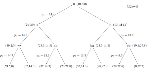
In the previous two examples, the effect associated with the addition of a bidder was subtle because the additional bidder failed to win any round of the auction. We now look into a case in which the additional bidder wins one auction round to verify if this is a sufficient condition for the seller’s revenue to increase with the number of bidders. Let us consider the following example where bidder A’s valuations for the objects are a120,
2 17
3 9.9
b , and bidder C’s valuations for the object are c1 15.5, c2 14.2, and c3 14.1.
Again, as in the previous two examples, bidder A has the three highest valuations.
Figure 4 illustrates the two-bidder auction involving bidders A and B. Solving the game shows that the equilibrium is unique and efficient as bidder A, with the three highest valuations, wins the object in all three rounds of the auction. The seller’s revenue when bidder C does not compete against bidders A and B is R(2) = 43, and the price path
(2) 14.4,14.3,14.3
P is weakly declining.
In contrast, the equilibrium price in the 3-bidder auction is constant: bidder C wins the first object at price 14.3 while bidder A wins the other two objects at the same price. By allowing bidder C to win the first object, bidder A does not have to contend with bidder C’s high valuation in the second and third rounds. This is the best possible outcome for bidder A when bidder C participates. But, bidder A’s gain in the 3-bidder auction is less than his gain in the 2-bidder auction (i..e, 8.4<10.5). The seller’s revenue is R(3) = 42.9, less than in the two-bidder auction involving bidders A and B.
PROPOSITION 2: In sequential second-price auctions under complete information with
two asymmetric bidders, the addition of a third bidder may decrease the seller’s revenue even when the third bidder wins an object.
Proposition 2 indicates that we cannot infer that the seller’s revenue increases by the addition of a new bidder from observing that the new bidder wins an object during the course of the auction. It is also worth noting that the tendency for the extra bidder to induce higher equilibrium prices in late rounds is not observed in this third example
because the competitive effects occur off the equilibrium path in the outcome tree. This is because bidder A maximizes its payoff by foregoing the first object, even though bidder A has the highest valuation for the first object. The strategy of bidder A removes the competitive effect associated with the extra bidder at the bottom of the outcome tree, and the addition of a bidder ends up having an adverse effect on the price of the first object.
Propositions 1 and 2 show ambiguous predictions regarding the effect of the addition of bidders on a seller’s revenue. Thus, it seems pertinent to look for additional insights from an empirical investigation. We investigate below the effect of adding bidders on the performance of Quebec’s electronic hog auction.
4. Background: Hog marketing mechanisms in Quebec
A provincial marketing board coordinates the marketing of hogs in Quebec. Provincial marketing boards in Canada market many commodities and vary greatly in terms of their powers and the policies and economic contexts under which they operate. A common objective of marketing boards in Canada is to offset the market power of downstream firms.5 This is particularly true for Quebec’s hog industry, whose 756 producers in 2011 (Statistics Canada, 2012), down from 3,322 in 1981, sell their hogs to 7 processors, the largest of which slaughters about two thirds of all the hogs produced in Quebec.
The creation of a marketing board with single-desk selling powers proved difficult in the Quebec hog industry (Larue, Gervais and Lapan, 2004). Quebec’s hog marketing board, the Fédération des Producteurs de Porcs du Québec (FPPQ) was established in
5
The empirical evidence reported in Fulton and Tang (1999) and Gervais and Devadoss (2006) suggests that producers are still at a disadvantage vis-à-vis downstream firms. Recent results about Canada’s chicken supply chain in Pouliot and Larue (2012) indicate that retailers carry more weight than processors, who in turn carry more weight than producers.
1981. A first daily electronic auction was introduced in 1989 to market all of the hogs produced in Quebec, including those owned by Quebec processors.6 Lower-than-expected prices led to various rule changes early on. By 1994, FPPQ added a second marketing mechanism to work concurrently with the daily hog auction.7 The share of the provincial hog supply marketed through the hog auction was reduced from 100% to 28%, and adjusted several times later.
In 2000, the FPPQ introduced a third concurrent marketing mechanism, an auction of monthly supplies. The share of hogs marketed through the daily auction remained at 25% from this point on. In a diminished role, the daily auction generated, more often than not, prices in excess of the US hog reference price; but there were times, when the North American hog-pork market was depressed, when it generated prices that were perceived as unreasonably low by the FPPQ. At different times the FPPQ invited processing firms from Ontario to participate in the auction, in hopes of inducing more aggressive bidding.
Ontario bidders still purchased most of their hogs in Ontario when invited to bid on the Quebec auction. Thus, their valuations for Quebec hogs must have been relatively low, or at least lower than if they had been consistently invited to bid on the Quebec auction. Typically, invitations to Ontario bidders were for one to three days. Furthermore, the proportion of Quebec’s hog supply marketed through the hog auction had also been
6
A contract between the FPPQ and the hog processors listed the responsibilities of the FPPQ and the processors as well as the rules of the auction. The processors agreed to buy all of the hogs marketed by the FPPQ and in exchange the FPPQ agreed to sell only to Quebec processors. As a result, Quebec remained a large exporter of pork meat while other provinces like Ontario and Manitoba exported more piglets and live hogs.
7
Hogs were formula-priced and supplies were allocated based on the volume slaughtered in the previous year by each processor. The base price was the US reference price adjusted for the exchange rate, a carcass weight differential and a discount factor.
substantially reduced after 1994, which meant that Ontario bidders could not realistically expect to secure large hog supplies from Quebec.
The merger of Quebec’s two largest hog processors in 2005 combined with declining prices in North America pressured auction prices down. The daily auction was temporarily shut down in October of 2006, but it resumed its activities in April of 2007, only to be permanently closed in February of 2009.
5.Empirical Evidence from the Quebec Daily Hog Auction
The FPPQ graciously provided us with the full data about daily auctions held in February, May, and August from 1995 to 2006, for a total of 402 observations. Thus, our sample covers only the period when the auction had a diminished role. The data include the id number of the winner of each round, prices, lot size, total number of hogs sold that day and the US reference price. Table 1 shows summary statistics of our data. Bidders from Ontario were invited 24 times to participate in the daily auction, consisting of 6% of the daily auctions for which we have data. Because we are interested in the seller’s revenue, our dependant variable is the average daily price, computed as the simple average of the prices for all of the lots auctioned on a given day. The mean and standard deviation for the (average daily) auction price (or AUCprice) indicates that it was quite volatile over the period covered by our sample. The same can be said about the US hog price.
In the period covered by the data, Quebec meat processing firms competed in the domestic output market, dominated by three large distributors/retailers, and in export markets, with the United States and Japan as the main destinations at the time. In addition, meat processors competed in a daily auction for the purchase of “virtual” hogs
scoring 100 on a quality index.8 The processing technology is well known and so were the processing firms’ plant sizes and costs for other inputs like labor, energy, and materials. These conditions are very similar to the ones described by Bernheim and Whinston (1986) to justify the modelling of auctions under complete information. Thus, we argue that complete information is not too heroic an assumption.
Given the short amount of time between auctions and the fact that a substantial fraction of Quebec’s hog supply was marketed through other marketing mechanisms, one could argue that a buyer’s share on the auction could vary from one day to the next as a smaller number of lots won on a given day could be compensated by a larger number of lots won the next. We believe that the scope for this kind of dynamic adjustment was limited. Processing facilities operate daily and a shortage in the supply of hogs can disrupt operations and significantly increase average processing costs.9 Processors prefer a stable procurement of hogs on a daily basis and this is why they were supportive of the pre-attribution system based on historical shares to work alongside the daily auction, even though this caused higher hog procurement cost for them (Larue, Gervais and Lapan, 2004).
In our sample, the Herfindahl index about daily allocations averages 0.286 (or 2,860)10 and it has a standard deviation of 0.073 (or 730). This small standard deviation shows that there have been variations in the allocated shares of individual bidders from one day to the next, but that these variations have been relatively small. Accordingly, lagged average auction prices might be warranted in our subsequent regressions, but
8
Delivered hogs were graded and deviations from the 100-score entailed a premium or a discount that was agreed upon between producers and processors. Hence, uncertainty over quality did not play a role.
9
Workers in Quebec hog processing facilities are unionized. Thus, given contracts with unions, processors have little flexibility in adjusting their labor force in the short run.
10
insights from our static examples are still relevant in the development of priors for our empirical analysis. Because Ontario bidders were not allowed to bid often and for several days in a row, they had to purchase the bulk of their hogs from other sources. The implication is that their valuations for Quebec hogs were residual valuations representing the profit that could be generated from processing additional hogs beyond their planned capacity. Under these circumstances, theoretical predictions as to whether the presence of Ontario processors had a positive or negative effect on the average daily auction price in Quebec are ambiguous, and the issue can only be settled through regression analyses.
OLS estimates
We wish to test whether inviting additional bidders had a positive or negative effect on the average daily price generated by the hog auction. We begin with a OLS model and then in the next section we account for endogeneity in the timing of invitations.
We regress the average daily price generated on Quebec’s hog auction (AUCprice) on the reference US daily hog price converted to Canadian dollars and adjusted for carcass size (USprice),11 the available daily quantity of hogs sold on the auction (quantity), and the presence or absence of additional bidders (Dinvited). In a second model, to verify the robustness of our results, we add dummy variables for seasonality (d_month) and year-fixed effects (d_year). We consider that quantity is exogenous as supplies of hogs are determined by decisions made months before slaughter. As hogs reach maturity, feedlots do not have other options than to send them
11
This US price was used by the FPPQ in the implementation of its pre-attribution mechanism which ran alongside the daily auction. The US price is considered as exogenous as changes in the volume marketed through the Quebec daily auction are not important enough to impact the US market.
for slaughter, regardless of prices, hence justifying the exogeneity of the quantity variable.
The regression equation for the model with season and year effects is
1 1 2 3 7 4 5 1 , t t t t t t yi ti t t i
AUCprice AUCprice USprice AUCquantity
DMay DAugust dYear Dinvited
(1)where t is a well-behaved error term. In reporting results below, we do not calculate the long-run effects implied by the presence of a lag dependent variable. The reason is that invitations to Ontario bidders were extended for short periods of time. Our interest is in the immediate effect of these invitations that were never meant to be permanent.
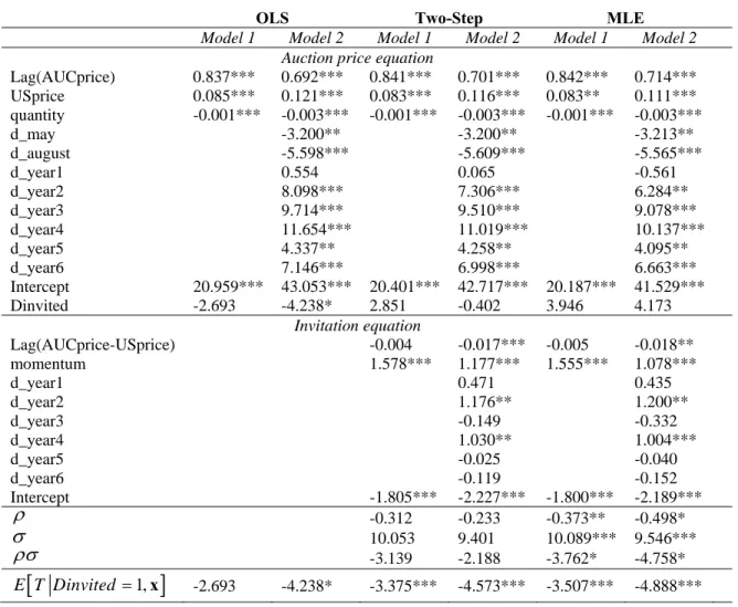
The first two columns of Table 2 summarize the OLS regression results. The coefficients on the lag price and US price have the expected positive signs, while the coefficient for the supply of hogs auctioned is negative, as expected. The sizes of the coefficients for the year dummies in the second model are quite variable, which is consistent with the volatility of the hog industry. The coefficients on the indicator variable about the presence of invited bidders are negative, but significant only in the second model. This suggests that prices were lower on the days when Ontario processors were invited to bid on the Quebec auction. Further analysis is required before a causal effect can be established.
The data show that Ontario processors did make some purchases when invited to bid on the auction, but that their share averaged only 6% of the volume sold on the days they bid. This suggests that Ontario processors’ highest valuations were tied to hogs from Ontario. Consequently, the anti-competitive effect discussed in proposition 2 cannot be ruled out. Still, the negative coefficient on the indicator variable does not necessarily
imply that the invited bidders caused the price to decline. The coefficient may embody an endogeneity bias sufficiently large to mask a positive causal relation from the number of bidders to the average auction price. A bias would be present if invitations had been extended only when prices were low. The possibility of declining prices causing increases in the number of bidders must be internalized in our econometric investigation.
Accounting for endogenous invitations extended to Ontario bidders
To account for endogeneity of invitations, we rely on a two-equation model which can be estimated by full maximum likelihood, or by a two-step approach pioneered by Heckman (1979). The model addresses the problem associated with invitations possibly not made at random dates. This procedure has been applied widely in the measurement of treatment effects and program effectiveness (Greene, 2008 p.889). We will estimate the two-equation model with both the two-step approach and the maximum likelihood estimator (MLE). In the MLE approach the equations are jointly estimated, but at the cost of more structure being imposed, because the residuals are assumed to be distributed according to a bivariate normal. The two-step approach yields estimates that are consistent, but less efficient than the MLE. The two-step procedure calls for a probit estimation from which we compute an Inverse Mills ratio for each observation and use it as an extra regressor/Heckman correction in the second equation. A drawback of this approach is that the correction term derived from the first equation and used in the second equation often relies on explanatory variables that are also in the second equation, which makes it harder to precisely estimate individual effects (Wooldridge, 2002, p.565). Because this
procedure is simple and well known, our description below will focus mainly on the MLE procedure.
The first equation models the decision of the FFPQ to invite Ontario processors to participate in the Quebec hog auction. This is the so-called selection component. In our case, the FFPQ likely extended invitations when the previous day’s auction price was low in relation to the US benchmark. This rationalizes the insertion of the one-day lagged difference between the auction price and the US price. We use a momentum variable, defined by a dummy variable that equals 1 when Ontario bidders were allowed to bid the previous day, to internalize the possibility of invitations for more than one day. In a second model, the equation also includes year dummy variables.
The second equation explains the auction price and is analogue to the OLS model in equation (1). The equation includes the dummy variable capturing the presence of Ontario bidders, a lagged auction price, the US price and, in a second model, seasonal dummies and year effects.
The two-equation model for the MLE can be represented as follows:
* * 1 , 1 0 , , t t t t t t t t t t Dinvited u Dinvited DinvitedAUCprice AUCprice Dinvited
α w β x (2)
where x and w are vectors of explanatory variables. Identification of the parameters in equation (2) is facilitated through exclusion restrictions of the variables for one-day lagged difference between the auction price and the US price, and the momentum variable from the auction price equation. The variables for the lag of the price, the US price, the quantity, and the months are excluded from the invitation equation. These exclusions are reasonable, in particular, because it is not price levels or quantities that
motivate invitations but rather the difference with US prices. Similarly, it is the US price and the auction price in the previous period that explains the auction rather than the difference between US and Quebec prices.
In the MLE, the errors and u have mean zero and are correlated with
covariance matrix typical of a selection model:
2 1 .
Defining Prob(Dinvited1|w) (α w , where )
. is the cumulative function for the normal distribution. Note that the sample selection model is not required when , or 00
. In such a case, OLS yields consistent parameter estimates.
The conditional expectations of the average auction price are given by: ( ) ( 1, ) , ( ) E AUCprice Dinvited α w x β x α w (3) ( ) ( 0, ) 1 ( ) E AUCprice Dinvited α w x β x α w . (4)
The difference between the two expectations is the variation in the average auction price due to the presence of Ontario bidders:
( 1, ) ( 0, )
1
T E AUCprice Dinvited E AUCprice Dinvited
x x α w α w α w (5)
Computing equation (5) is still relevant even if the null of 0 is not rejected at the conventional significance level. In particular, as previously mentioned, inference about the correction term in the two-step approach is likely to be affected by multicollinearity. The measure in equation (5) remains an accurate estimate of the effect of extending
invitations to Ontario bidders even if multicollinearity affects our estimates. Because we hypothesize that bidders were invited under “special” circumstances, we compute the treatment effect only for observations when invitations were extended to Ontario bidders. We then take the average and report the average treatment effect on the treated
1,
E T Dinvited x. Note that the average treatment effect in the OLS model is the
coefficient for the invitation dummy.
The last four columns of Table 2 report the results of the two-equation model. As in the OLS estimates, we report short-run effects as invitations to participate in Quebec auction were never meant to be last more than a few days. The bottom of Table 2 displays coefficients from which we can infer whether the Dinvited dummy variable is endogenous in the price equation. In the two-step procedure, is not statistically different from zero at the 10% confidence level in both models. In the MLE, , and
are statistically significant at the 10% level or less.
Overall, the evidence that the timing of invitations exactly coincided with spells of low prices is supported by the MLE estimators, but not by the two-step estimators. The hypothesis that invitations extended to Ontario bidders when prices were low is intuitive, but because these invitations occurred very rarely, their empirical significance is harder to establish. The FFPQ had a contract with Quebec hog processors, arbitrated by the Quebec government, which legally constrained its ability to sell hogs to out-of-province buyers. Furthermore, because out-of-province buyers could not consistently rely on Quebec hogs to meet their slaughtering capacities, they may not always have been in a position to purchase hogs when the FPPQ contacted them.
In both model 1 and model 2, the magnitude and signs of most of the coefficients in the auction price equation are very robust across estimators. If it was not for the differences in the coefficients pertaining to the invitations, this could be construed as additional evidence that invitations were perhaps random events. The significance of the coefficients for the lagged auction price in the price equations confirms that shocks on the auction price were not instantaneously transmitted, but the transmission was still fairly quick given the size of the coefficient. The US price and quantity coefficients are statistically significant and have the expected respective positive and negative signs. The size of the coefficients on the invitation dummy varies significantly across models, and the same can be said about the estimates of . However, coefficient estimates for the invitation variable are most robust across models when the MLE estimator is used. As a result, we believe that the MLE estimator can better characterize the effect of adding bidders on the average daily auction price.
We compute the treatment/invitation effects, T E AUCprice Dinvited( x1, )
( 0, )
E AUCprice Dinvited
x , using equation (5) for observations for which
Dinvited=1 and report the average. All estimates of the invitation effect are negative and
only in the OLS estimate of model 1 is the effect not statistically significant. The effect of invitation in auction price is smaller in model 1, where it varies between 3.507 and -2.693. In model 2, the estimates of the invitation effect varies between -4.888 and -4.238. The treatment effects are surprisingly robust across estimators even though the coefficients for the invitation dummy varied a lot across estimators. Overall, using a median range of our estimates of E T Dinvited 1,x, we find that extending an
invitation to Ontario bidders lowered the average price at the daily auction by about $3.50–$4.
To put these estimates in perspective, the average auction price (over the lots auctioned during a day) varied between a low of $110 and a high of $220 per 100 kg in our sample. Thus, we find that the effect of extending invitations to Ontario had a small negative effect as it lowered the price by only a few percentage points. However, this small negative effect occurred when prices were already low. On average, the auction price when Ontario bidders were invited was $14 below the average for the overall sample. Furthermore, the FPPQ had high hopes that the added competition would boost prices. Our results show that these invitations had the perverse effect of lowering prices. The previous section shows that competition amongst completely informed bidders can produce a negative invitation effect. We are confident that our econometric estimates capture such an effect. The usual suspect behind unexpected price reductions, collusion, was never considered by FFPQ to be the cause of lower prices in Quebec auctions, because the largest buyer was a cooperative.
6. Summary and Conclusion
This article investigates the effect of increasing the number of bidders in livestock auctions. We show that in sequential multi-unit auctions under complete information, a setting consistent with the working of livestock auctions, a seller’s revenue may increase or decrease when additional bidders are allowed to participate. Previous work also shows a negative relationship between the number of bidders and the average auction price, but not in contexts that fit with the specifics of livestock auctions.
The existence of an anti-competitive effect from adding bidders to an auction hinges on new bidders affecting the ranking of the highest valuations for an object. In some cases, even if valuations for an object are higher with the addition of bidders, the average price in sequential multi-unit auctions may decline as the bidders change their bidding strategies. We show that an additional bidder can exert a negative effect on the seller’s revenue even if he does not win a single object. Furthermore, observing that the additional bidder wins one object is neither necessary nor sufficient for a positive effect on the seller’s revenue. Such adverse effects have been documented by others under different theoretical assumptions (e.g., Mathews, 1984; Menicucci, 2009), but not under complete information. We did not find well-documented empirical evidence in support of this peculiar effect.
Our empirical analysis focuses on Quebec’s daily hog auction that involved only a few bidders/meat processors from Quebec, except under special circumstances when bidders from Ontario were invited. The Quebec hog auction used a structure that is very similar to other livestock auctions in North America. We find robust evidence across econometric models that the participation of Ontario bidders in the Quebec auction had a negative effect on auction prices.
Ontario bidders source their hogs mainly in Ontario and as a result had low marginal valuations when invited to bid on the Quebec auction. Still, Ontario bidders mattered in Quebec’s daily auctions as Ontario processors won some lots of Quebec hogs. However, as our theoretical examples show, the introduction of new bidders tends to increase competition down the outcome trees in late auction rounds, but this ends up impacting bidders’ behavior in early rounds with prices for the first objects possibly
declining enough to induce reductions in the average price/seller’s revenue. We infer from this that the presence of additional bidders induced Quebec hog processors to revise their bidding strategies in a way to cause declines in the average daily auction price.
Finally, our findings shed new light on competition in livestock markets. In particular, we show that auction prices are not a monotonic and increasing function of the number of bidders. It is not only the number of bidders that matters in determining equilibrium auction prices. The ranking and differences between the valuations of the bidders is also crucial. An implication is that in markets with great heterogeneity among a few buyers, which is common in agriculture given the high levels of concentration in processing activities, marketing alternatives to auction might yield better prices to sellers. For policy analysis of the livestock industry, an implication of our results is that traditional models of imperfect competition, such as the Cournot model, are not appropriate to approximate the outcome of auctions.
7.
References
Ausubel M., Milgrom, P., 2002. Ascending Auctions with Package Bidding. Frontiers of
Theoretical Economics 1: No. 1, Article 1.
http://www.bepress.com/bejete/frontiers/vol1/iss1/art1
Baumol, W.J., Panzar J.C., Willig R.D., 1982. Contestable Markets and the Theory of Industry Structure. New York, NY: Harcourt Brace Jovanovitch.
Bernheim, B. D., Whinston M. D., 1986. Menu Auctions, Resource Allocation, and Economic Influence. Quarterly Journal of Economics 101, 1-32.
Crespi, J. and Sexton, R. 2004. Bidding for Cattle in the Texas Panhandle. American
Journal of Agricultural Economics 86, 660-674.
Elmaghraby, W. J., 2005. The Effect of Asymmetric Bidder Size on an Auction’s Performance: Are More Bidders Always Better? Management Science 51(12), 1763-1776.
Fulton, M. and Tang, Y. 1999. Testing the Competitiveness of a Multistage Food Marketing System: The Canadian Chicken Industry. Canadian Journal of
Agricultural Economics 47, 225–250.
Gale I. L., Stegeman M., 2001. Sequential Auctions of Endogenously Valued Objects.
Games and Economic Behavior 36, 74-103.
Gervais, J.P. and Devadoss, S., 2006. Estimating Bargaining Strengths of Canadian Chicken Producers and Processors Using a Bilateral Monopoly Framework.
Agribusiness 22, 159-173.
Gervais, J.P. and Lambert, R., 2010. The Simple Economics of Hog Marketing Reform in Quebec. SPAA working paper #2010-01.
Greene, W. H., 2008. Econometric Analysis. Sixth Edition, Prentice Hall, Upper Saddle River NJ.
Heckman, J., 1979. Sample Selection Bias as a Specification Error. Econometrica 47, 153-161.
Jeddy M., Larue, B., Gervais J-P., 2010. Allocations and Price Trends in Sequential Auctions under Complete Information with Symmetric Bidders. Economics Bulletin 30, 429-436.
Jeddy M., Larue B., 2012. Multiplicity of Equilibria in Sequential Auctions with Asymmetric Bidders. Economics Bulletin 32, 456-465.
Katzman B., 1999. A Two Stage Sequential Auction with Multi-Unit Demands. Journal
of Economic Theory 86, 77-99.
Kittsteiner, T., Nikutta J., Winter E., 2004. Declining Values in Sequential Auctions.
International Journal of Game Theory 33, 89-106.
Krishna, K., 1993. Auctions with Endogenous Values: The Persistence of Monopoly Revisited. American Economic Review 83, 147-160.
Krishna, K., 1999. Auctions with Endogenous Values: The Snowball Effect Revisited.
Economic Theory 13, 377-391.
Larue, B., Gervais, J.P. and Lapan, H.E. 2004. Low-Price Low-Capacity Traps and Government Intervention in the Quebec Hog Market. Canadian Journal of
Agricultural Economics, 52,3 :237-256
Matthews, S.A., 1984. Information Acquisition in Discriminatory Auctions. In: Boyer, M. Kihlstrom, R.E. (eds.) Bayesian Models in Economic Theory, pp. 181-207. North-Holland, New York.
Menicucci, D., 2009. Competition May Reduce the Revenue in a First Price Auction with Affiliated Private Values. The B.E. Journal of Theoretical Economics Volume 9: Issue 1 (Advances), Article 38.
Milgrom, P., 2004. Putting Auction Theory to Work. Cambridge University Press, Cambridge, UK.
Mishra, D., Reddy S.S., Veeramani D., 2005. Performance Evaluation of Multi-Object Auctions. Electronic Commerce Research 5, 293-307.
Pinkse, J., Tan G., 2005. The Affiliation Effect in First Price Auctions. Econometrica 73, 263-277.
Pouliot, S. and Larue, B. 2012. Import Sensitive Products and Perverse Tariff-Rate Quota Liberalization. Canadian Journal of Economics, 45,3:903-924.
Rong, Z., Zhi-xue, L., 2007. Two-Stage Procurement Auction with Bidders of Asymmetric Capacity. System Engineering-Theory and Practice 27, 36-41.
Statistics Canada, 2012. 2011 Census of Agriculture.
http://www.statcan.gc.ca/daily-quotidien/120510/dq120510a-eng.htm (consulted on January 30, 2013).
Wooldridge, J.M., 2002. Econometric Analysis of Cross Section and Panel Data. MIT Press, Cambridge MA.
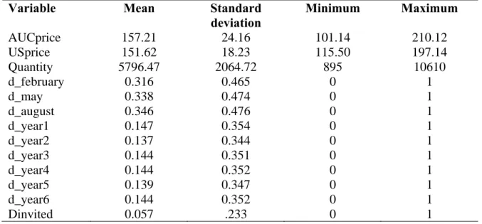
Table 1. Summary data
Variable Mean Standard
deviation Minimum Maximum AUCprice 157.21 24.16 101.14 210.12 USprice 151.62 18.23 115.50 197.14 Quantity 5796.47 2064.72 895 10610 d_february 0.316 0.465 0 1 d_may 0.338 0.474 0 1 d_august 0.346 0.476 0 1 d_year1 0.147 0.354 0 1 d_year2 0.137 0.344 0 1 d_year3 0.144 0.351 0 1 d_year4 0.144 0.352 0 1 d_year5 0.139 0.347 0 1 d_year6 0.144 0.352 0 1 Dinvited 0.057 .233 0 1
Table 2. Regressions prices generated by the Quebec hog auction
OLS Two-Step MLE
Model 1 Model 2 Model 1 Model 2 Model 1 Model 2
Auction price equation
Lag(AUCprice) 0.837*** 0.692*** 0.841*** 0.701*** 0.842*** 0.714*** USprice 0.085*** 0.121*** 0.083*** 0.116*** 0.083** 0.111*** quantity -0.001*** -0.003*** -0.001*** -0.003*** -0.001*** -0.003*** d_may -3.200** -3.200** -3.213** d_august -5.598*** -5.609*** -5.565*** d_year1 0.554 0.065 -0.561 d_year2 8.098*** 7.306*** 6.284** d_year3 9.714*** 9.510*** 9.078*** d_year4 11.654*** 11.019*** 10.137*** d_year5 4.337** 4.258** 4.095** d_year6 7.146*** 6.998*** 6.663*** Intercept 20.959*** 43.053*** 20.401*** 42.717*** 20.187*** 41.529*** Dinvited -2.693 -4.238* 2.851 -0.402 3.946 4.173 Invitation equation Lag(AUCprice-USprice) -0.004 -0.017*** -0.005 -0.018** momentum 1.578*** 1.177*** 1.555*** 1.078*** d_year1 0.471 0.435 d_year2 1.176** 1.200** d_year3 -0.149 -0.332 d_year4 1.030** 1.004*** d_year5 -0.025 -0.040 d_year6 -0.119 -0.152 Intercept -1.805*** -2.227*** -1.800*** -2.189*** -0.312 -0.233 -0.373** -0.498* 10.053 9.401 10.089*** 9.546*** -3.139 -2.188 -3.762* -4.758*
1,
E T Dinvited x -2.693 -4.238* -3.375*** -4.573*** -3.507*** -4.888***Notes: Statistical significance is not calculated for and in the two-step approach, but is calculated for the product . Statistical significance are denoted by * p < 0.10, **
Figure 1. Outcome tree for 2-bidder auction in example #1.
Notes: At each node, the gross payoffs in parenthesis are identified from left to right to bidders A and B respectively. Arrows denote the allocation in each subgame and prices are given next to the paths.
Figure 2. Outcome tree for 3-bidder auction for examples #1 and #2.
Notes: At each node, the gross payoffs in parenthesis are identified from left to right, or from top to bottom, to bidders A, B and C respectively. Arrows denote the allocation in each subgame and prices are given next to the paths.
Figure 3. Outcome tree 2-bidder auction for example #2.
Notes: At each node, the gross payoffs in parenthesis are identified from left to right to bidders A and B respectively. Arrows denote the allocation in each subgame and prices are given next to the paths.
Figure 4. Outcome tree for 2-bidder auction for example #3.
Notes: At each node, the gross payoffs in parenthesis are identified from left to right to bidders A and B respectively. Arrows denote the allocation in each subgame and prices are given next to the paths.
Figure 5. Outcome tree for 3-bidder auction for example #3.
Notes: At each node, the gross payoffs in parenthesis are identified from left to right, or from top to bottom, to bidders A, B and C respectively. Arrows denote the allocation in each subgame and prices are given next to the paths.


![[PDF] Cours générale sur la programmation en C++ | Cours informatique](data:image/gif;base64,R0lGODlhAQABAIAAAP///wAAACH5BAEAAAAALAAAAAABAAEAAAICRAEAOw==)