The hydrodynamics associated with instream large roughness elements in gravel-bed rivers = L'hydrodynamique associée aux éléments de rugosité dans les rivières à lit de graviers

Université de Montréal

The hydrodynamics associated with instream large roughness elements in gravel-bed rivers

(L’hydrodynamique associée aux éléments de rugosité dans les rivières à lit de graviers)

par R.W. Jay Lacey

Département dc géographie faculté des arts et des sciences

Thèse présentée à la Faculté des études supérieures en vue de l’obtention du grade de

Philosophiae Doctor (Ph.D.) en géographie

Décembre, 2007

ï

Dc

v

oDI

Université

de Montréal

Direction des bib1othèques

AVIS

L’auteur a autorisé l’Université de Montréal à reproduire et diffuser, en totalité ou en partie, par quelque moyen que ce soit et sur quelque support que ce soit, et exclusivement à des fins non lucratives d’enseignement et de recherche, des copies de ce mémoire ou de cette thèse.

L’auteur et les coauteurs le cas échéant conservent la propriété du droit d’auteur et des droits moraux qui protègent ce document. Ni la thèse ou le mémoire, ni des extraits substantiels de ce document, ne doivent être imprimés ou autrement reproduits sans l’autorisation de l’auteur.

Afin de se conformer à la Loi canadienne sur la protection des renseignements personnels, quelques formulaires secondaires, coordonnées ou signatures intégrées au texte ont pu être enlevés de ce document. Bien que cela ait pu affecter la pagination, il n’y a aucun contenu manquant.

NOTICE

The author of this thesis or dissertation has granted a nonexciusive license allowing Université de Montréat to reproduce and publish the document, in part or in whole, and in any format, solely for noncommercial educational and research purposes.

The author and co-authors if app!icabte retain copyright ownership and moral rights in this document. Neither the whote thesis or dissertation, nor substantial extracts from it, may be printed or otherwise reproduced without the author’s permission.

In compliance with the Canadian Privacy Act some supporting forms, contact information or signatures may have been removed from the document. While this may affect the document page count, it does flot represent any loss of content from the document.

Univesité de Montréal faculté des études supérieures

Cette thèse intitulée:

The hydrodynarnics associated with instream large roughness elements in gravel-bed rivers

(L’hydrodynamique associée aux éléments de rugosité dans les rivières à lit de graviers)

présentée par: R.W. Jay Lacey

a été évaluée par un jury composé des personnes suivantes:

Lael Parrott- présisent-rapporteur

André Roy - directeur de recherche

Michel Lapointe—codirecteur dc recherche

Pascale Biron- membre du jury

Jan Reid - examinateur externe

lii

RESUMÉ

Cette thèse constitue une étude de la distribution spatiale hydrodynamique autour des éléments larges de rugosité (ÉLRs) tel que les amas de galets et les blocs erratiques dans les rivières à lit de graviers. Les ÉLRs sont les éléments microtopographiques les plus fréquents dans les rivières à lit de graviers peu triées. Ils semblent être distribués aléatoirement dans le chenal et augmentent la stabilité du lit. Le transport de sédiments est diminué par l’imbrication des ÉLRs avec le substrat environnant, limitant la disponibilité de particules transportables et retardant leur mouvement initial. Il a été montré que les ÉLRs fournissent un habitat qui est préféré par les poissons; cependant, les raisons qui expliqueraient cette relation positive n’ont pas été clairement identifiées.

À

ce jour, aucune étude à notre connaissance n’a examiné l’hydrodynamique in situ à une échelle fine autour des ÉLRs submergés; une telle investigation permettra d’améliorer notre compréhension du rôle que jouent les ÉLRs dans l’hydrodynamique à échelle locale et à échelle de la rivière ainsi que dans l’habitat aquatique. Les objectifs spécifiques de cette thèse sont: 1) d’identifier et de quantifier l’effet de l’échelle spatiale sur les variables de turbulence de l’écoulement obtenues à partir d’un plan vertical au-dessus d’un ÉLR en utilisant des techniques statistiques multivariées; 2) de caractériser le champ d’écoulement tridimensionnel (3D) in situ avec et sans un ÉLR submergé isolé et d’analyser l’effet hydrodynamiqtie des ÉLRs sur les structures turbulentes d’écoulement à grande échelle (GÉ); 3) de décrire et de quantifier en détail les couches de cisaillement des ÉLRs et les processus d’échappement associés ainsi que le comportement des structures d’échappement à échelle moyenne sous l’influence des structures d’écoulement à GÉ; 4) de déterminer l’effet de conditions d’écoulement variées (niveau d’eau et composante de vitesse longitudinale moyenne) et de la géométrie des ÉLRs (forme, grosseur, orientation) sur le champ d’écoulement turbulent 3D in sUit et sur l’échange de momentum turbulent.

Cette thèse intègre l’utilisation de plusieurs techniques complémentaires déchantillonnage sur le terrain et d’analyses statistiques pour atteindre les objectifs présentés et obtenir une caractérisation détaillée du champ d’écoulement autour des ÉLRs dans les rivières à lit de graviers. Jusqu’à quatre vélocimètres acoustiques Doppler

(ADVs) ont été utilisés pour les mesures de vitesse 3D à haute fréquence. Des mesures 2D précédemment obtenues à partir de courantomètres électromagnétiques (ECM5) ont également été analysées pour répondre à l’objectif Ï. Une technique nouvelle de mesures simultanées provenant d’ADVs synchronisées avec la visualisation de l’écoulement a été utilisée pour résoudre l’objectif 3, permettant l’étude détaillée de la couche de cisaillement des ÉLRs et des structures d’échappement associées. Des analyses statistiques multivariées ont été utilisées pour étudier les relations d’échelle dans les données spatialement distribuées et également pour trouver des relations fonctionnelles entre l’écoulement moyen et les variables morphométriques des ÉLRs et les variables turbulentes estimées à partir de la zone de sillage.

La quantification de patrons spatiaux à différentes échelles a été obtenue par l’utilisation d’une analyse canonique de redondance (RDA) et d’une analyse de coordonnées principales des matrices de voisinage (PCNM). La RDA, très exploité dans le domaine de l’écologie, est rarement utilisée dans le domaine des ressources d’eau. L’analyse PCNM est une méthode nouvellement développée de partitionnement statistique basée sur les échelles; son utilisation dans cette thèse est une première application pour les sciences de ressources de l’eau. Cette analyse a été faite à partir d’un plan vertical de mesure au-dessus d’un ÉLR. Les analyses présentées dans les chapitres subséquents de cette thèse utilisent des plans de mesures horizontaux permettant d’évaluer adéquatement l’importance de l’influence hydrodynamique latérale des ÉLRs. Les changements dans le champ d’écoulement induits par un ÉLR isolé ont été évalués par l’échantillonnage des vitesses dans deux plans horizontaux avec et sans un ÉLR. Des analyses spectrales et de corrélations croisées (espace-temps) ont permis la quantification de la périodicité des structures d’échappement dans la couche de cisaillement et le comportement des structures cohérentes d’écoulement à GÉ lors de leur passage au-dessus d’un ÉLR. La technique de mesures simultanées provenant des ADVs et de la visualisation de l’écoulement a été utilisée pour identifier le comportement de l’échappement et de la couche de cisaillement au passage d’évènements d’écoulement à GÉ. Alors que la partie précédente de cette thèse étudiait des ÉLRs isolés pour évaluer l’influence hydrodynamique spécifique associée à un ÉLR, la dernière partie de la thèse porte sur plusieurs ÉLRs de différentes géométries sous des

V

conditions découlement variées. finalement, les implications de cette thèse sont discutées dans un contexte plus large, abordant des enjeux en géomorphologie fluviale et des enjeux qui concernent l’habitat des poissons.

Les principaux résultats de cette thèse montrent que les ÉLRs génèrent une turbulence 3D intense dans la zone de sillage avec des valeurs extrêmes des indicateurs principaux de turbulence (par exemple l’énergie cinétique turbulente, ke, et le cisaillement de Reynolds) 5 — 10 fois plus grandes que les valeurs non obstruées. Ces

valeurs élevées se présentent dans une zone relativement localisée en dessous du sommet des ÉLRs et directement en aval des ÉLRs. La zone turbulente de sillage a été montrée comme étant bien structurée par la taille de l’ÉLR et par la vitesse longitudinale non obstruée moyenne, qui explique plus de 70 — 80% de la variance de k et du

cisaillement longitudinal-vertical de Reynolds, —pïtW. Un processus bimodal

d’échappement a été observé en aval des ÉLRs, où des vortex d’instabilité initiale à échelle fine s’amalgamaient à intermittence en des structttres d’échappement plus grandes à échelle moyenne avec des fréquences d’échappement d’approximativement de 5 Hz et 1 Hz, respectivement. La fréquence d’échappement des structures d’écoulement à échelle moyenne correspondait approximativement aux valeurs prédites à partir du nombre de Strouhal. Les valeurs de cisaillement de Reynolds élevées sont apparues selon des patrons particuliers dans la zone de sillage des ÉLRs. Des valeurs de cisaillement longitudinal-latéral (uv) de Reynolds élevées, —pi, ont formé des zones allongées +ve et —ve en aval, attribuées à des vortex tournant en sens contraire le long de l’axe vertical s’échappant des côtés latéraux du ÉLR. Des valeurs élevées de —puw ont

été observées occupant la plus grande partie de la zone de sillage apparaissant conctirremment avec des valeurs élevées de —pïï et sotivent dominant l’échange de

momentum turbulent. Utilisant la visualisation simultanée de l’écoulement, les valeurs élevées de —piTi ont été directement associées à des vortex latéraux s’échappant du

sommet des ÉLRs. L’interaction entre les strtictures de la couche de cisaillement et les structures cohérentes d’écoulement à GÉ a été observée comme étant intermittente. Les structures d’écoulement à GÉ ont été montrées comme étant relativement peu affectées par les structures d’échappement, alors qu’à l’opposé les structures de la couche de cisaillement ont été observées s’échappant à intermittence vers le haut et se contractent

vers le lit avec le passage respectif des éjections et des incursions à GÉ. L’étude de l’hydrodynamique in situ à échelle fine autour des ÉLRs présentée dans cette thèse contribue à élucider le rôle des ÉLRs dans les rivières à lit de graviers et sera profitable aux domaines de la géomorphologie fluviale, de l’ingénierie en rivière et de la biologie aquatique.

Mots Clés turbulence; éléments de rugosité; amas de galets; ADV; visualisation; structures turbulentes d’écoulement; statistiques multivariées; spectrales; spatiales; corrélations croisées; vortex; habitat aquatique; lit de graviers.

VII

SUMMARY

This thesis investigates the spatially distributed hydrodynarnics associated with submerged large roughness elements (IREs) such as boulders, cobbles and pebble clusters in gravel-bed rivers. Instream LREs have been argued to constitute the most frequent microtopographic feature in poorly sorted gravel-bed rivers. These features appear to be randomly distributed over the channel bed and have been found to enhance bed stabiÏity. Reduced bedload fluxes are associated with LREs, as they interlock and imbricate with the surrounding substrate limiting the availability ofreadily transportable particles and delaying their incipient motion. LREs have been shown to provide preferred habitat for fish, yet the reasons for this positive relationship are flot clear. To date, no studies to our knowledge have examined the fine-scale in situ hydrodynamics around submerged IREs, the detailed investigation of which will advance the understanding of the role LREs play in local and river hydrodynamics and aquatic habitat. The specific objectives ofthis thesis are: I) to identify and quantify the spatial scale-dependence of turbulent flow variables obtained from a vertical plane crossing over a IRE through the use of multivariate statistical techniques; 2) to characterise the in sitti 3D turbulent flow field with and without an isolated subrnerged LRE and investigate the hydrodynamic effect of LREs on large-scale (LS) turbulent flow structures advecting from upstream; 3) to describe and quantify in detail IRE shear layers and associated shedding processes and the behaviour of meso-scale shedding structures under the influence ofLS flow structures; 4) to determine the effect ofvaried flow conditions (stage and mean longitudinal component velocity) and of LRE geometries (shape, size, orientation) on the in situ 3D turbulent flow fïeld and turbulent momentum exchange.

This thesis integrates the use of multiple complementary field sampling instrumentation techniques and statistical analyses to fulfil the outlined objectives and obtain a comprehensive characterization of the flow field around LREs in gravel-bed rivers. Mtiltiple acoustic Doppler velocimeters (ADV5) were the primary instruments used for 3D high-frequency velocity measurements. Previously obtained 2D meastirements from electrornagnetic current metres (ECM5) were also analysed to

address objective 1. A novel technique of concurrent ADV measurements with flow visualization was used to accomplish objective 3 permitting a detailed investigation of the L’RE shear layer and associated flow structures. Multivariate statistical analyses were used to investigate scale relationships in the spatially distributed data as well as to find functional relationships between rnean flow and LRE morphometric variables and turbulence variables estimated from the wake.

The quantification of scale-dependent spatial pattems was obtained through the use of canonical redundancy analysis (RDA) and principal coordinates of neighbour matrices (PCNM) analysis. RDA, while commonly used in ecology sciences, is rarely used in the field of water resources. PCNM analysis is a newly devetoped rnethod of statistical scale partitioning and its use in this thesis represents a first time application to water resotirce sciences. This analysis was carried out on a vertical measurement plane crossing over a LRE. Subsequent chapters of this thesis focussed on horizontal measurement planes to properly assess the importance of the lateral hydrodynamic influence of LREs. Changes in the flow field induced by an isolated IRE were assessed by sampling velocities over two horizontal planes with the LRE present and resampling identical locations after the LRE was removed. Spectral and space-time correlation analyses provided a quantification of shear layer periodicity and a characterization ofthe behaviour ofdownstream advecting LS turbulent coherent flow structures as they passed overtop of the LRE. The concurrent ADV measurements and flow visualization technique was used to identify shedding and shear layer behaviour to the passage ofLS flow events. While the preceding portion ofthe thesis focused on isolated LREs in order to assess the hydrodynamic influence specifically associated with a LRE, the latter portion ofthe thesis focused on multiple LREs with different geometries under varying flow conditions. This allowed for a more generalized description of the hydrodynamic influence of LREs. Finally, the implications of the thesïs for broader fluvial geomorphological issues and fish habitat were discussed.

The main results ofthe thesis show that LREs generate intense 3D turbulence in the wake with peak values in the main turbulent indicators (e.g., turbulent kinetic energy, ke, and Reynolds shear stresses) 5 — 10 times greater than free-stream values.

ix

downstream ofthe LREs. Wake turbulence was shown to be well structured by LRE size and mean free-stream longitudinal velocity which cxplained upwards of 70— 80% ofthe variance in ke, and longitudinal-vertical Reynolds shear stress, —ptïW. A bimodal

shedding process vas observed in the 1cc of LREs where srnall-scale initial instability vortices intermittently amalgamated into larger meso-scale flow structures with shedding frequencies of approximately 5 Hz and 1 Hz, respectively. The shedding frequency of the meso-scale flow structures corresponded adequately to predicted values using a Strouhal number of 0.1$. Elevated Reynolds shear stresses occurred in particular patterns in the wake of LREs. High longitudinal-lateral Reynolds shear stress —pïiî

occurred in downstream elongated +ve and —ve zones attributed to counter rotating vertical axis vortices shedding from the lateral sides of the LRE. High —p was observed to occtipy much of the wake occurring over large scales Ax 5h — 10h

concurrently with high —piïîY and ofien dom inating the turbulent momentum exchange.

Using the concurrent flow visualization the high —pi7i and turbulent events were directly associated with lateral axis vortices shedding from the top of the LREs. The interaction between the shear layer structures and LS coherent flow structures was observed to be intermittent. LS flow structures were shown to be relatively unaffected by LRE shedding flow structures, while conversely the shear layer structures were seen to intermittently shed upwards and contract downwards towards the bed with the passage of LS ejections and sweeps, respectively. The fine-scale in situ hydrodynamics around LREs characterised in this thesis provide valuable insight on the role ofLREs in gravel-bed rivers which will be helpftil for the fields of fluvial geomorphology, river engineering and aquatic biology.

Key words: turbulence; large roughness elements: pebble clusters; ADV; visualization; coherent flow structures; variation partitioning; spatial; spectral; space-time correlation; multivariate analysis; shear layer; vortices; aquatic habitat; gravel-bed rivers.

TABLE 0F CONTENTS

RÉSUMÉ iii

SUMMARY vii

TABLE 0F CONTENTS x

LIST 0F TABLES xïii

LIST 0F FIGURES xiv

LIST 0F SYMBOLS xxi

DEDICATION xxiii

ACKNOWLEDGEMENTS xxiv

1. INTRODUCTION 1

2. BACKGROUND 4

2.1.Context 4

2.1.1. Boundary layer theory over srnooth and rough beds 5

2.1 .2. Turbulence intensities, correlations, macroscales and spectra li

2.2. Turbulent coherent flow structures 1 8

2.2.1. Turbulent coherent flow structures in srnooth and rough boundary layers..19 2.2.2. Large-scale turbulent coherent flow structures 23 2.2.3. Coherent turbulent flow structures in shear layers 29

2.2.3.1.MixingÏayers 29

2.2.3.2. Isolated bÏiffbodies— awayfrom the wall 30

2.2.3.3.Backwardfacing steps, dunes and wallpositioned bhiffbodies 33

2.2.4. Shedding frequency 40

2.3. Large roughness elernents in gravcl-bcd rivers 44

2.3.1. The spatial distribution of large roughness elernents 45

2.3.2. Large roughness elernent hydrodynamics 46

2.4. Large roughness elements and aquatic biota 52

2.4.1. Periphyton 52

2.4.2. Benthic invertebrates 54

2.4.3.Fish 55

3. OBJECTIVES AND METHODOLOGY 61

3.1. Problem Staternent 61

3.2. Objectives 63

3.3. Approach and General Methodology 65

3.3.1.In situ velocity measurements 68

3.3.2. Measurernents of instantaneous velocities synchronous with digital video

recordings 72

3.4. Conclusion 73

4. SPATIAL SCALE PARTITIONING 0f INSITUTURBULENT FLOW DATA

OVER A PEBBLE CLUSTER IN A GRAVEL-BED RIVER 76

4.1. Introduction ₇₆

xi

4.3. PCNM statistical analysis .83

4.4. Results 88

4.4.1. Global PCNM model RDA $8

4.4.2. PCNM submodels RDA $9

4.4.3. PCNM submodel multiple regressions 89

4.4.4. Spatial decomposition and intercorrelation of PCNM submodel flow

variables 91 4.4.4.1. Veiy-Ïarge-scaÏe submodeÏ 93 4.4.4.2. Large-scate submodeÏ 95 4.4.4.3. Meso-scale submodel 97 4.4.4.4. Fine-scaÏe subrnodel 97 4.5. Discussion 9$ 4.6. Conclusions 101

5. A COMPARATIVE STUDY 0F THE TURBULENT FLOW FIELD WITH

AND WITHOUT A PEBBLE CLUSTER IN A GRAVEL-BED RIVER 104

5.1. Background 104

5.2. Field Measurernents 106

5.3. Data Treatment and Anatysis 108

5.4. Results 114

5.4.1. Turbulence statistics 115

5.4.2. Spectral Analysis 119

5.4.3. Frozen turbulence hypothesis 122

5.4.4. Length scales, integral time scales and correlation structure lengths 123

5.5. Discussion 12$

5.6. Conclusions 131

6. FINE-SCALE CHARACTERIZATION 0F THE TURBULENT SHEAR

LAYER 0F AN INSTREAM PEBBLE CLUSTER 134

6.1.Introduction 134

6.2. Methods 136

6.2.1. f ield Measurements 136

6.2.2. Data treatment 138

6.3. Results 141

6.3.1. Time-averaged mean and turbulence statistics 141

6.3.2. Spectral analysis 143

6.3.3. Correlation analysis 145

6.3.4. Quadrant analysis 147

6.3.5. Skew and kurtosis coefficient analysis 150

6.3.6.Visualization 151

6.4. Discussion 154

6.5. Conclusions 157

7. THE SPATIAL CHARACTERIZATION 0F TURBULENCE AROUND

LARGE ROUGHNESS ELEMENTS IN A GRAVEL-BED RIVER 159

7.2. field Measurements .161

7.3. Data Analysis and Treatment 163

7.3.1. Redundancy analysis 166

7.4. Results 169

7.4.1. Bed topography and LRE rnorphometrics 169

7.4.2. Flow conditions and turbulent wake statistics 170

7.4.3. Spatial distribution of turbulent parameters 173

7.4.4. Redundancy analysis 1 79 7.5. Discussion 186 7.6. Conclusions 191 8. IMPLICATIONS 193 8.1. Sedimcnt transport 193 8.2. Spatial Organization 199

8.3. On the origin and maintenance ofLS coherent flow structures 201

8.4. Fish habitat 202

8.5. Conclusions 210

9. GENERÀL DISCUSSION AND CONCLUSIONS 211

9.1. Summary ofthe key flndings 211

9.2. Towards a better understanding ofLRE hydrodynamics 213

9.3. Originality ofthe thesis 217

9.4. future rescarch 21$

BIBLIOGRAPHY 220

APPENDIX A -ACCORD DES COAUTEURS ET PERMISSION DE L’ÉDITEUR

234 APPENDIX B -AUTORISATION DE RÉDIGER LA THÈSE SOUS FORME

XIII

LIST 0F TABLES

Table 2.1. Dimensions of large-scale flow structures (modifïed fromRoy et aÏ. [2004])...

2$

Table 4.1. Spatial means and standard dcviations ofthe flow variables 83 Table 4.2. Scale classification ofthe significant PCNM variables $7 Table 4.3. Estimated fractions of unadjusted variance (R,2) of flow variables expressed by significant canonical axes (Only significant canonical axes of each submodel are presented). The bottom row presents the unadjusted canonical eigenvalues (2) of each significant axis (2 are estimated as the mean R,2 value for aIl 15 response variables); and the far right colurnn presents the unadjusted coefficients of multiple determination (R2)

using aIl 29 significant PCNMs. Monte Carlo significance test (999 unrestricted

permutations) 94

Table 5.1. Spatial averages (and standard deviations) of the mean and turbulent flow parameters for each plane of measurements and in the case of the cluster being presdnt

orrernoved 116

Table 5.2. Spatial averages (and standard deviations) of I and 1*, for each plane of measurernents and in the case ofthe cluster being present or removed 11$

Table 5.3. Mean advcction velocity and spatially averaged mean ITS for each plane of measurements and in the case ofthe cluster being present or removed 123

Table 6.1. Skcwness and kurtosis coefficients and intermittency factors for u, w and ztw

tirne series estirnated from eight centerline measurement locations aty= O andz = 0.9.

151

Table 7.1. Large roughness element morphometrics and mean flow variables 16$

Table 7.2. Correlation coefficients, r, between the LRE morphometrics and mean flow

variables for the upper and lower planes 171

Table 7.3. Turbulence variables in the wake ofLREs 172

Table 7.4. Correlation coefficients, r, between the turbulence variables in the wakc

region for the upper and lower measurement planes 172

Table 7.5. Marginal effects (individual explained variance) of LRE rnorphometrics and

mean flow variables 181

Table 7.6. Conditional effects (additional explained variance) ofexplanatory variables... 181

Table 7.7. Estimated fractions of unadjusted variance (R,2) of turbulence variables

expressed by canonical axes I, II and full model I $2

Table 7.8. Partitioned lower measurement plane submodels — estirnated fractions of

unadjusted variance (R,2) of turbulence variables expressed by canonical axes and full

LIST 0f FIGURES

Figure2.1. Boundary layer structure for shallow open channels 5

figure 2.2. Variation of turbulent intensities,

L,

over smooth and rough beds as a function of relative height z/Z for a range of dimensionless roughness values. k [Nezu

andNakagawa, 1993J 12

figure 2.3. Correlation coefficients R for a range of dirnensionless roughness values,

k [NezuandNakagawa, 1993] 14

Figure 2.4. Distributions of macroscale L, as a function of z/Z for a range of

dimensionless roughness values, k [Nezu andNakagawa, 1993] 15

Figure 2.5. u component velocity spectra (a) for seven depths over a rough-bed [Noweli and Church, 1979]. (b) for a gravel-bed river under bedload movement flow conditions. The heavy line represents the spectrum for the lowest sensor in the array (lowest z/Z)

[Dinehart, 1999] 17

Figure 2.6. Plan view ofstreak structure ofa flat plate turbulent boundary layer close to

the wall at z =2.7 [KÏine et al., 1967] 20

Figure 2.7. Conceptual smooth-bed model of streaks, ejections and sweeps [Smith,

1996] 21

Figure 2.8. Conceptual fully-rough bed model of the generation of hairpin vortices

[$mith, 1996] 22

Figure 2.9. Images extracted from a flow visualization sequence in the gravel-bed river. The 2.5 s visual sequence illustrates the passage of a high-speed wedge followed by a low-speed wedge which takes the form ofa violent ejection [Roy et aÏ., 2004] 23

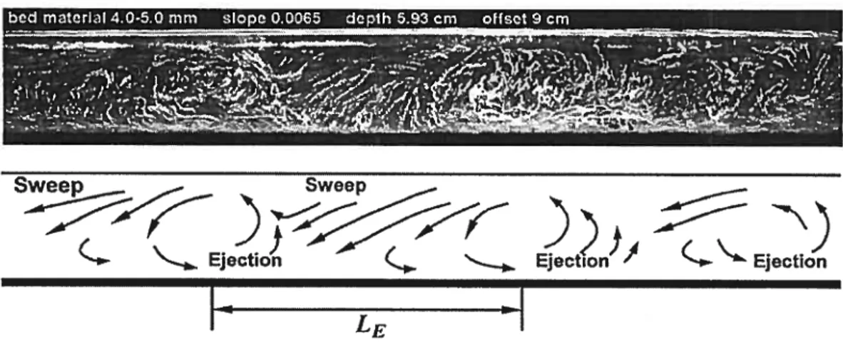
Figure 2.10. Visualization of large-scale turbulent structure of open-channel flow over mobile gravel beds (camera is moving with mean flow velocity). f low is right to lefi.

[Shvidchenko and Fender, 20011 24

figure 2.11. Conceptual model of LS turbulent coherent flow structures [$hvidchenko

andFender, 2001] 25

figure 2.12. Conceptual model of LS turbulent coherent flow structures formation

process [Khii andAdrian, 19991 26

Figure 2.13. PIV of large-scale structure of hairpin vortex packets at Re 7705. The solid lines are contours of constant longitudinal velocity at 61% and 79% of the free stream velocity. Grey levels indicate swirling strength and flow is from left to right

[Adrianet al.. 2000] 26

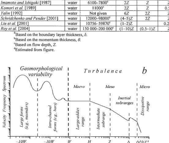
figure 2.14. Schematised velocity spectra in gravel-bed rivers retated to scating parameters. (note: W0. W H, Z, and are defined here as river valley and river channel widths, flow depth, height above the bed, and grain size, respectively) [Nikora, 20071

xv Figure 2.15. Schematic ofshear mixing layer between two parallel flows with different

mean velocities

t7Ç

and

U

29

Figure 2.16. Pairing mechanism of shearïng vortices

_[

Winant andBrowand, 1974] 30 Figure 2.17. InitiaI shear layer instability vortices: (a) smoke visualization in the wake of a sphere, Re0 = i0 [Taneda, 197$]; (b) PIV contours of positive and negative

vorticity in the wake ofa cylinder, Re0 [Lin et aï., 1995]. f low is from lefi to right 33 Figure 2.1$. Numerical 2D LES of shear layer instability vortices and drag crisis for a cylinder placed in flow. Close-up view of either side ofthe cylinder. Flow is from left to right. Drag crisis is observed for Re 106 subplot where the wake is significantly narrowed and separation ofthe initial instability vortices is delayed further downstream

along the cylinder. [$ingh andliittal, 2005] 33

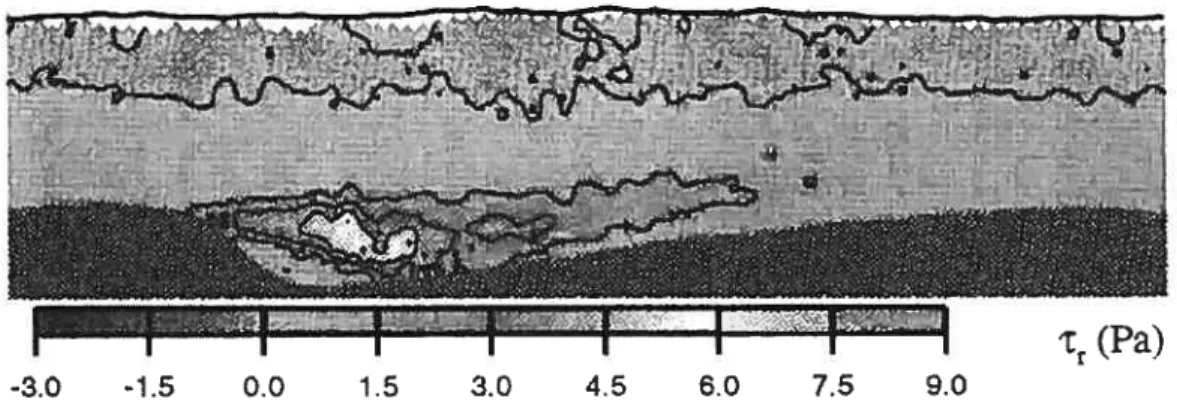
Figure 2.19. Backward facing step features [Nezu andNakagmva, 1989] 34 Figure 2.20. Contour rnap of —pïïW over a dune, Re 5.7 x I 0. Flow is from left to

right. [Bennett andBest, 1995] 35

Figure 2.21. Flow separation model and interaction with LS coherent turbulent structures. D denotes detachment location. Vre denotes the mean re-entrainment velocity. Dotted line denotes

U=

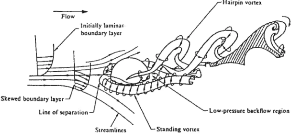
0. Solid une denotes maximum —iïW [Sirnpson et al., 1981]

36 Figure 2.22. Conceptual model offlow over a grounded hemisphere in a laminar flow at

Re0 3400[AcarlarandSmith, 1987] 37

Figure 2.23. Bed pressure coefficients surrounding an isolated hemisphere at Re0 = 5.2

x I [Brayshaw et al., 1983] 3$

Figure 2.24. Drag coefficient for varying longitudinally aligned hemisphere separation

distances [Brayshmv et aï., 1983] 39

Figure 2.25. Velocity power spectra obtained from two types of shear layers: a) river confluence, Re i05 [Rhoads andSztkhodoïov, 2004]; b) dune —flume experiment, Re =

2500 [Kadota andNezu, 1999J 43

figure 2.26. Pebble cluster bedform [Brayshmv, 1984] 45 Figure 2.27. Conceptual model offlow over a pebble cluster based on detailed velocity measurements over a dense sampling grid [Bzffin-Bélanger andRoy, 1998] 4$ Figure 2.2$. The centrality offlow wedges in the dynamics offlow in a gravel-bed river

[Roy and Bz4fin-BéÏanger, 2001] 51

Figure 2.29. Integrated channel scale modet presenting the interaction between LS flow structures, ejections and shedding structures [3zffin-3élanger et al., 2001 b] 51 Figure 2.30. Periphyton biomass versus shear velocity, ït,, at the sedirnent-water

interface [Hondzo and Wang, 2002] 53

Figure 2.31. Time series (ms) of trout body outlines superimposed onto vorticity and velocity vector plots ofthe cylinder wake [Liao et al., 2003b] 57

Figure 2.32. Fish locations relative to the locations of bricks for discharges of(a) 0.030 and (b) 0.111 rn3 s1. Ftow is from lefi to right [Smith et aï., 2005] 59 Figure 3.1. Schernatic ofgaps in knowledgebase (unanswered questions) regarding LRE hydrodynamics and the respective objectives of this thesis used to answer these

questions 65

Figure 3.2. Support frarne and ADV configurations for the experiments conducted in a) Chapter 5 and b) Chapter 7. Flow is from left to right 69 Figure 3.3. a) ADV and underwater digital camera aluminium stipport frame, 1.5 m x 1 .5 ni; b) schematic of experimental set-up for synchronous visualization and velocity

measurements [Lacey and Roy, 2007bJ 71

Figure 4.1. Sampling x-z transect plane with measurement points (dots). Modified from

Btffin-Bélanger and Roy[1998] $0

Figure 4.2. x-z transect plot of standardized vaLues (z-scores) of the mean and turbulent flow statistics: a)

U

b)

W

c) u’ d) w’ e) —pïiW

f)

5k1, g) Sk1 h) TQ2TIo i) TQ4ThO

j)

TQ2TI12 k) TQ4Th2 l)fQ2Yh2ITI)fQ4Th2 n) ITS,, o) ITS11,. Positive values are represented by filled bubbles, negative values by empty bubbles. Bubble size indicates relative magnitude. Flow is from lefi to right. Modified from3zffin-Bélanger andRoy [1998]

82 Figure 4.3. Methodotogy for developing PCNM variables. a) Example of sampling locations with Euclidian links between coordinates; b) Euclidian distance (D1) matrix; c) truncated D1 matrix (neighbouring matrix) truncated at d 1 .0 by dm; d) principal coordinate (eigenvector) matrix, indicating positive, zero and negative eigenvalues; e) examples of PCNMs (positive eigenvalued principal coordinates) representing very large (PCNM 1), large (PCNM 5), meso (PCNM 13) and fine (PCNM 37) scales. The size of the bubbles is proportional to the magnitude of the PCNM variable values (positive values filled). f low is from lefi to right. f) Response (flow) matrix and explanatory (PCNM) matrix used in multiple regression and canonical analysis.

Modified from BorcardandLegendre [2002] $6

Figure 4.4. Fraction of explained variance (unadjusted coefficient of multiple determination, R2) for individual mean and turbulent flow variables, for each significant PCNM submodel (p< 0.05): very-large (VL), large (L), meso (M) and fine (F) scale...90 Figure 4.5. Significant canonical axes ofthe “fitted site scores” (p <0.05) plotted on the sampling location coordinates. a) VL-axisl; b) VL-axis2; c) L-axisl; d) L-axis2; e) L axis3; f) L-axis4 g) M-axis 1; h) M-axis2; i) F-axis 1. Positive values are represented by fi lied bubbles. The right-hand bar graphs present the fraction of variance for each flow variable explained by the canonical axes (empty negative correlations, filled

positive). Flow is from left to right 92-93

Figure 4.6. Eigenvector scatter plots. Canonical axis I is the abscissa while canonical axis 2 is the ordinate. a) VL-scale b) L-scale c) M-scale d) F-scale 95 Figure 5.1. a) Upstream view of the Eaton North River; b) Aluminium support frame with 4 ADVs (flow is ftom left to right); c) Side view ofpebble cluster; d) Same view as

xvii

Figure 5.2. Plan view ofthe frame and ofthe sampiing locations. The sampling strategy ofthe velocity fluctuation measurements used fotir ADVs simultaneously. it consisted of three series of measurements at two different sampling planes at relative heights ofz/Z= 0.2 and z/Z= 0.4 respectively. A probe remained stationary at the front of the ciuster

during ail three series at a given height above the bed while the three other probes were iocated systematically further downstream. Ail indicated distances on the diagram are in

metres. f low is from lefi to right 108

Figure 5.3. a) Bed topography elevations; b) Photo composite of the bcd. The pebble cluster can be seen in the central left portion of both images. Black dots represent sampling locations ofthe velocity measurements. f low is from left to riglit 115

Figure 5.4. Spatial distributions of u’, y’ and w’ values for the planes oC measurement

and for the cases with and without the pebble cluster. Black dots represent sampling locations ofthe velocity measurements. Flow is from left to right 117 Figure 5.5. The spatial distributions for each measurement plane and for both cases, with and without the pebble cluster, of a) Turbulent kinetic energy, ke; b) Longitudinal velocity turbulent intensity, I. Black dots represent sampling locations of the velocity

measurements. Flow is from lefi to right 118

Figure 5.6. Spatially averaged wavenumber spectral density, <Sa>, for each

measurement plane. The spectra are scaled by u. and z 120

figure 5.7. Spectral density, S, for the measurement plane at zIZ 0.2, with and without the pebble cluster. The spectral sequence starts downstream ofthe lee side edge

ofthe pebble cluster and it follows along the centerline 121

Figure 5.8. Comparison of the length scales obtained from the autocorrelation, _R(At), and spatial-time correlation, R(Ax,Ay=OEAt=0.25), analyses for ail three velocity components measured at two planes above the bed with and withoutthe cltister 123

Figure 5.9. a) Longitudinal velocity integral time scale (ITS,,); b) U-level analysis indicating the frcquency of high-speed (HS) and low-speed (LS) events. Black dots represent sampling locations ofthe velocity measurements. Flow is from lefi to right

125

Figure _{5.10. Space-time correlation, R(Ax,Ay,At), function diagrams for the a)}

longitudinal; b) lateral; c) vertical velocity components at time lags, At = 0.25s, 0.5s,

I .Os, I .5s, and 2.Os. The spatial patterns are given for both measurement planes and for both cases, with and without the pebble cluster. Only significant correlations are represented(ci 0.05). Flow is from left to right in each sub-plot _127-128

Figure 6.1.Bed topography; (a) Plan view; (b) Side view. Black dots represent sampling locations ofthe velocity measurements. Flow is from lefi to right (modified from Lacey

andRoy [20061) 137

Figure 6.2. Plan and side views of turbulent kinetic energy ke. Black dots represent sampling locations of the velocity measurements. Flow is from lefi to right. Cluster

Figure 6.3. Plan and side views of mean Reynolds shear stresses, —pz7W. Black dots

represent sampling locations of the velocity measurements. Flow is ftom left to right.

Cluster location is represented by thick black une 143

Figure 6.4. Velocity power spectra, S,,(j) and coherency squared spectra, y,

_(f).

The spectra are estimatcd at measurement locations: (a-b) (-2.4,0,0.9); (c-d) (1.2,0,0.9); (e-f) (1.8,0,0.9); (g-h) (1.2,-0.9,0.9);

(i-j)

(1.8,-0.9,0.9) 144

Figure 6.5. Plan and side views ofu component integral time scale, ITS11. Black dots represent sampling locations of the velocity measurements. Flow is from left to right.

Cluster location is represented by thick black une 146

Figure 6.6. Plan and side views of (a) u component maximum space-timc correlations,

Ruu(AX,AY,AZ,Atmax). Between measurements at x -0.4 m and ail downstream

measurements and (b) between measuremdnts at x = 0.1 m and ail downstream

measurements. Black dots represent sampling locations of the velocity measurements. Flow is from lcft to right. Cluster location is represcnted by thick black une 147

Figure 6.7. Fractional contribution of quadrants to local mv compondnt mean Reynolds

stress, —pïW, for hole sizes, H= O (solid lines) and H= 2 (dashed unes). Lec edge of

cluster is positioned at x = 0. Estimates arc for eight measurement points along the

centerliney =O atz =0.9 for eight longitudinal locations x -2.4, x = 0.6, x 1.2,

x 1.5, x = 1.8,x 2.4, x 2.9, and x =6.2 148

Figure 6.8. Distribution of maximum -pmi’ per Q2 and Q4 event at two hole sizes H O

and H 2. Box-plots estirnate measurement points along the centerline v= O at =0.9

for eight longitudinal locations x =-2.4, x =0.6, x = 1.2, x = I.‘,x = 1.8, x 2.4,X

= 2.9, and x = 6.2. Cross points represent extreme values beyond 3 times the

interquartile range. Frequencies of occurrence are presentcd at the top of each box-plot 149 Figure 6.9. -puw versus frequency of Q2 and

Q4

events.(a-b) Average _{maximum -p}ttw per event, —puw , versus frequency of occurrence. (c-d) Sum of-puw per cvcnt at

each frequency of occurrence. Estimates are for measurement points along the centerline

O atz 0.9 for six longitudinal locations x -2.4, x 0.6, x 1.2, x 1.5, x=

2.4,andxr6.2 ₁₅₀

Figure 6.10. Digital image pairs, separated by Ai, presenting characteristic shedding behaviour: (a-b) shedding of individual initiai instability vortices. mode 1; (c-d) pairing

oftwo _{initiai instability vortices; (e-f) formation and shedding of h scaled structures,} mode 2. f low is from left to right. Arrow indicates tracer injection location 152

figure 6.11. (a) Sequence of 6 enhanced images detailing the behaviour of the shear layer with the passage of LS ejection structures advecting from upstream fort = 0.4 s; t

0.7 s; t = 1.0 s; t 1.2 s; t = 1.4 s; t 1.7 s; (b) -pmv time series for measurement

positions x -2.4, x 0.6, and x = 1 .2. Quadrant 2 and Qtiadrant 4 contributions are

presented as dark and pale circles, respectively. The x -2.4 time series. has been synchronized with the x 0.6 location. f low is from lefi to right. Arrow indicates tracer

xix figure 6.12. (a) Sequence of 6 enhanced images detailing the behaviour of the shear layer with the passage ofLS swecp and ejection structures advecting from upstream fort = 0.6 s; t = 0.8 s; t = 0.9 s; t 1.1 s; t 1.3 s; t = 1.5 s; (b) -puw time series for

measurement positions x -2.4, x = 0.6, and x 1.2. Quadrant 2 and Quadrant 4

contributions are presented as dark and pale circles, respectively. The x = -2.4 time

series, has been synchronized with the x = 0.6 location. f low is from left to right.

Arrow indicates tracer injection location 154

Figure 7.1. Plan view of bed topography: (a) Site 3, (b) Site 5, (c) Site 7, (d) Site 2, (e) Site 8, (f) Site 10. Black dots represent sampling locations ofthe velocity measurements. Flow is from lefi to right. LRE x-y cross-section plotted as thick black une 163 Figure 7.2. Turbulent kinetic energy, ke, at Sitc7C for the upper and lower measurement x-y planes. Black dots rcpresent locations of the velocity measurements. f low is ftom lefi to right. Cross-hatching indicates the LRE location 174 Figure 7.3. Turbulent kinetic cnergy, ke, at Site 2, Site $ and Site lOB for thc lower measurerncnt x-p planes. Black dots represent sampling locations of the velocity measurements. Elow is from lefi to right. Cross-hatching indicates the LRE location

174 figure 7.4. Spatial distributions of the u component integral time scale, ITS1, at Site 2, Site 8 and Site 1 OB for the lower measurcmentx-yplanes. Black dots represent sampling locations of the velocity measurernents. Flow is from left to right. Cross-hatching

indicates the LRE location 175

Figure 7.5. Scatter plot of LRE wake lateral width, Øwk, as a ftinction of LRE lateral width. Ø. Open circles represent uppcr plane measurements and fllled triangles represent lower plane measurernents. Dashed line indicates 1:1 ratio 176 Figure 7.6. Reynolds shear stresses at Site 3 for the upper and lower measurementx-y planes. Black dots represent sampling locations of the velocity mcasurements. Flow is from left to right. Cross-hatching indicates thc LRE location 177 Figure 7.7. Spatial distribution of: (a) —pTiY; and (b) —pzfW at Site 5A,B,C for the

upper and lower measurement x-y planes showing variability with river stage under flow conditions: A: Z 0.45 rn, = 0.57 m 51; B: Z= 0.51 m,

U

0.70 m s1; C: Z=

0.57 m,

U

0.85 m s1. Black dots represent sampling locations of the velocity measurements. Flow is from left to right. Cross-hatching indicates the LRE location

17$ Figure 7.8. Bivariate scatter plots of: (a) &tke vs. Z; (b) kemax vs. Ø (c) —piiï vs.

0.5ApU2. Open circles represent upper plane measurements and fllled triangles

represent lower plane measurements 179

Figure 7.9. RDA correlation biplots for ail sites estimates from: (a) upper measurement plane model, (b) lower measurement plane model. Canonical axis I is the abscissa while canonicat axis Il is the ordinate. Dashed vectors explanatory (independent) variables while solid vectors are time-averaged turbulent (response) variables I $4

Figure 7.10. RDA correlation biplots for lower measurerndnt plane model controlling for: (a) Ø — submodel J; (b) Z and

U1

— submodel 2. Canon ical axis I is the abscissa

while canonical axis II is the ordinate. Dashed vectors explanatory (ïndependent) variables while solid vectors are tirne-averaged turbulent (response) variables 185 Figure 8.1. Spatial distribution of: a) bed topography; b) —pi7W at z = 0.12 m; e)

—piW at z 0.04 m at Site 8. Black dots represent sampling locations ofthe velocity measurements. f low is from lefi to right. LRE location represented by thick black line

and cross-hatching 195

Figure 8.2. Site topography. Black triangle and dots represent sampling profile locations. Triangle represents JAS holding location. Flow is from lefi to right 205

Figure 8.3. Spatial distribution of

U,

ke and ITS1, for depth averaged values; and values estimated at z0 = 0.06 m; and at _ZLOC 0.025 m. Black triangle and dots represent

sampling locations of the vclocity measurements. Triangles represents JAS holding location. Flow is from lefi to right. LRE location is outlined by black line 205

Figure 8.4.

U,

ke and ITS,1 scatter plots. Triangles represents JAS holding location. .20$ Figure 9.1. Schematic integrating and summarizing salient results on the hydrodynamic

xxi

LIST 0F SYMBOLS

A5 lateral projection area, m2. A,5k planar wake area, m.

cor-La, coherent flow structure correlation length-scale, u component, longitudinal direction,x, m.

D50 median grain size, m.

f frequency,s’.

fr

Darcy-Weisbach friction factor. f50 half-power frequency, s.

g gravitational acceleration, m s2.

h, maximum pebble cluster height, m.

h, large roughness element protrusion height, m. I velocity turbulent intensity.

L shear velocity turbulent intensity. I. image intensity time series.

ITS,,, ITS,., ITS,,, integral time scale, u,y,and w components, s. k wavenurnber, cm’.

ke turbulent kinetic energy, cm2 s2. k, equivalent sand roughness, m. K, Kurtosis coefficient.

L turbulent macro-scale, u component, m

L,,k wake length, rn.

p probability.

r correlation coefficient. r2 coefficient ofdetermination.

R2 unadjusted coefficient of multiple determination Can R2 unadjusted bimultivariate redundancy statistic

adj usted bimultivariate redundancy statistic.

Re. Reynolds shear number.

Rh hydraulic radius, m. R,, autocorrelation coefficient.

R,, time-shifted cross-correlation coefficient. Sk, Skewness coefficient.

S,, water surface slope.

S,, spectral density function, cm2 s’.

u, r,

W time-averaged longitudinal, lateral and vertical velocity, cm s1. zi,y, w instantaneous longitudinal, lateral and vertical velocity, cms1.

u’,y’,w’ root mean square of the longitudinal, lateral and vertical velocity fluctuations,

cms.

u, shear velocity, cm s1.

mean advection velocity ofcoherent structures, cms1.

x, y, longitudinal, lateral and vertical distance, m.

x,y, dimensionless longitudinal, lateral and vertical distance Z mean water depth, m.

characteristic roughness length, m. u statistical significance level.

boundaiy layer thickness, m. time step, s.

Ax, Ay,A longitudinal, lateral and vertical separation distance, m.

ke longitudinal separation distance to maximum ke, m.

canonical eigenvalues. intermittency factor.

o arbitraiy velocity component, cm252,

—piT5 ,—piT —p7 uv, uivandvwcomponent mean Reynolds shear stress, N m2.

r,, bed shear stress, N m2.

y kinematic viscosity, m2 s’.

p water density, kg m3.

°vk roughness element and wake lateral width, m. overbar temporal mean values.

angled parentheses<> _{spatial mean values.}

xxiii

DEDICATION

This thesïs is dedicated with much love to my father Alan Michael Lacey (1941-2007) who encouraged me wholeheartedly throughout my studies and who would have Iiked to have seen me finish.

Rage, rage against the dying ofthe light, Do not go gentie into that good night

ACKNOWLEDGEMENTS

J’aimerais tout d’abord remercier André Roy pour m’avoir accueilli, malgré un laboratoire déjà bien rempli, et guidé à travers l’incroyable aventure que fut mon doctorat. Conduire mes recherches en rivière naturelle fut une expérience riche et unique. Pour tous ses conseils judicieux et pour l’énergie, le souci du détail et la rigeur avec lesquels il a corrigé mes articles et résumés, peu importe le délai (parfois très court). Merci également pour les nombreuses opportunités de présenter mes travaux dans des congrès internationatix et le support financier durant les dernières années.

J’aimerais aussi remercier mon codirecteur de recherche Miche! Lapointe et les membres de mon comité doctoral, Pascale Biron et Lad Parrott, pour leur direction et pour les nombreuses discussions et réunions. J’aimerais remercier Pierre Legendre pour rendre le monde des statistiques multivariées si passionant et aussi accessible, et pour sa disponibilité durant mon doctorat. Aussi merci à Daniel Borcard pour les discussions sur les PCNM. Merci à Tom Buffin-Bélanger pour la permission d’utiliser ses anciennes données et pour ses commentaires sur une version préliminare du Chapitre 3. Thanks to Richard Allix the senior machine shop technician at Concordia University who fabricated my very solid ADV support frame which was fundamental to my in situ sampling.

Merci au groupe fluvial, le laboratoire était pour moi un endroit joyeux, favorable au travail et aux discussions, surtout les vendredis “fluviaux” à 16:00 (qui tout de même auraient pci être les jeudis). Thanks to my pal Bruce MacVicar for our fruitful discussions, Matlab collaborations and oh...1 don’t recail. Hélène Lamarre and Eva Enders for questions asked and answered. Special thanks to Geneviève Marquis for field, visualization and general aIl round help and conference partner. I would like to thank my numerous field helpers without whom this research would flot have taken place, Éric Beaulieu, Valérie Champagne, Lara Hoshizaki, Julie Thérien, Mathieu Roy, Christine Rozon.

xxv

Et finalement.j’aimerais aussi remercier Rosalie Léonard, qui m’a enduré pendant toute mathèse. Qui m’a supporté mentalement, physiquement, pour quelques scans ici et là, et pour plusieurs plusieurs traductions. Qui avec son regard positif et son immense patience m’a aidé à passer à travers tes moments difficiles (quand rien n’aboutit) et les multiples difficultés qui font d’un doctorat un doctorat.

t would like to thank the National Sciences and Engineering Research Council of Canada for the doctoral scholarship I was awarded, without which I would most likely flot be in research. J’aimerais également remercier la Faculté des Études Supérieures de l’Université de Montréal pour la bourse fin de doctorat. Funding for this research vas provided by the National Sciences and Engineering Research Council of Canada as well the Canadian foundation for Innovation. This research was conducted as part of the program ofthe Canada Research Chair in fluvial dynamics.

Turbulence is a ubiquitous characteristic of flows occurring in natural environments: from atmospheric flows to the flow of water in oceans and rivers. Turbulent flows are three dimensional and are characterised by high levels of fluctuating vorticity. In gravel bed rivers the turbulent velocity fluctuations in the fiow are driven by shear with the bed or through flow separation in the lee of bluff bodies. The turbulence is strongly influenced by the heterogeneous substrate made up ofdiscrete particles which protrude randomly from the bed. Significant feedbacks exist between the turbulent boundary layer structure, the bed microtopographic features and sediment transport [Leeder,

1983]. Grains and bedforms exert a significant influence on the flow and may greatly modify the turbulent boundary layer structure [Best, 1993]. The role of particle roughness and protrusion on the structure of the turbulent flow becomes increasingly important when the particles are large enough to create their own flow field capable of influencing erosion, transportation and deposition of other grains [Best, 1996]. These large roughness elements (LREs) consisting ofboulders, cobbles or pebble clusters form an integral part of the substrate and are considered to be the most prevalent microtopographic feature ofpoorly sorted gravel-bed rivers occupying as much as 10% of the channel floor [Brayshaw, 1984]. LREs play an important role in the local and global hydrodynamics of the river. They have been found to enhance bed stability and reduce bedload fluxes as they interlock and imbricate with the surrounding substrate limiting the availability of readily transportable particles and delaying their incipient

motion [Dal Cm, 1968; Brayshaw, 1984; Reid et aÏ., 1992; Biggs et aÏ., 1997;

Wittenberg andNewson, 2005]. While their spatial distribution is for the most part non periodic or quasi-random [Brayshaw, 1984;Lamarre andRoy, 2001], it has been argued that their spatial arrangement maximizes flow resistance [Hassan and RelU, 1990]. LREs in gravel-bed rivers have as well been associated with higher salmonid fish densities believed to be an effect of the heterogeneous flow conditions they impart [Van ZylÏ de Jong et aÏ., 1997;MitcheÏl et aÏ., 1998].

While the general effects of submerged LREs on flow resistance and benefits to fish habitat in flumes or in gravel-bed rivers have been investigated, several fundamental

2 questions remain on the hydrodynamic influence of LREs in gravcl-bed rivers and the role they play for aquatic biota. LREs generate complex three-dimensional (3D) turbulent flow patterns that very few studies have investigated in situ. Many questions need to be elucidated on: the spatial scales of turbulence generated; the two-dimensional (2D) and 3D spatial pafterns and extent of the hydrodynarnic effect; the details of the shedding processes; the effect of flow stage and changing LRE geometry on the hydrodynamics; and the interaction of LREs with large-scale (LS) coherent structures. LS flow structures are a predominant feature of gravel-bed rivers and through their associated sweeps and ejections play an important role in sediment transport and entrainment [WiÏliams et aÏ., 1989]. furthermore conflicting resuits in the biological literature have arisen on the effects of turbulence such as generated by LREs and fish [Enders et al., 2003; Smith et aÏ., 2005; 2006; Liao 2007]. These differences in resuits are difficuit to reconcile without a full understanding of the fine-scale 3D hydrodynamics associated with LREs in gravel-bed rivers. Through innovative in sittt

sampling techniques and turbulent data analyses this thesis is an attempt to advance current knowledge on the fine-scale in situ 3D hydrodynamics of submerged LREs in gravel-bed rivers.

This thesis is composed of eight chapters. A general review of the basics of turbulent flow over smooth and rough boundaries, turbulent coherent flow structures, LRE hydrodynamics and aquatic biota interactions with LREs is given in Chapter 2. This review presents and discusses past and current knowledge of turbulent flow processes associated with LREs in gravel-bed rivers and helps situate the objectives and results of this thesis within the broader gravel-bed river context. The detailed thesis objectives and methodology are presented in Chapter 3. The main results ofthe thesis are presented in Chapters 4 through 7. These chapters are written in journal article publication format for submission to internationally recognized research journals. Liaison paragraphs are included between the article chapters. Chapter 8 examines the broader implications ofthe thesis results for gravel-bed rivers and aquatic biota.

The chapters presenting new results are organized as follows: In Chapter 4 we quantify the spatial scale dependence of turbulent flow parameters in a longitudinal vertical, x-z plane, crossing over a naturally occurring pebble cluster in a gravel-bed

river. The scale dependent spatial patterns are obtained through the use of multivariate statistical techniques: canonicat redundancy analysis (RDA) and principal coordinates of neighbour matrices (PCNM) analysis. RDA, while commonly used in ecological sciences, is not oflen used in the field ofwater resources. Chapter 4 shows the utility of RDA and PCNM anatysis to investigate retationships between spatially distributed turbulence variables over a LRE which have a broad range of applications in water resources and earth sciences. The application ofthis technique will reveal the dominant scales at which turbulence manifestations occur. This article is now published in Water

Resoïtrces Research. In Chapter 5, the horizontal distribution of turbulent flow parameters over and around an isolated LRE in a gravel-bed river is characterised over two longitudinal-lateral (x-y) planes. Spectral and space-time correlation analyses are used to quantify shear layer periodicity and the response of advecting LS turbulent coherent flow structures to the mesoscale flow structures shedding from the LRE shear layer. The main results of this article are now published as a technical note in Water

Resources Research. In Chapter 6, concurrent flow visualization and 3D velocity measurements are used to investigate the fine-scale characteristics ofthe shear layer and shedding coherent flow structtires of an isolated in situ LRE. Through the concurrent measurement technique, identified turbulent flow events can be visually characterised leading to a better understanding of the turbulent flow processes occurring in the lee of LREs. Due to the fine-scale characterization and the extensive turbulent flow statistical analysis this article vas submitted and has now been accepted for publication by the

Journal ofHydrauÏic Engineering. In Chapter 7, several isolated and multiple LREs are investigated in a gravel-bed river under varying flow conditions. RDA is used to identifj the dominant flow parameters for structuring the turbulence generated in the wake. The investigation of several LREs at varying flow stages allows for a more generalized description of the hydrodynamic influence of LREs. This article will be submitted to GeoniorphoÏogy. Chapter $ explores the implications of the findings reported in the thesis for four particular areas: sedirnent transport, the channel-scale spatial distribution of LREs, LS coherent turbulent flow structures and fish habitat. A general conclusion establishes the contribution ofthe thesis and proposes directions for future work.

4

2.

BACKGROUND

2.1. Context

In gravel-bed rivers, the hydrodynamics are strongly influenced by the heterogeneous topography of the bed resulting from the arrangement of discretc particles of various shape, size and orientation. Secmingly distributed at random locations, the large roughness elements (LREs) are cither isolated boulders or cobbles or are the aggiomeration and imbrications of several large or small particles such as in pebble clusters or in ribs or steps. As these LREs protrude from the bed, they have a potentially stronger influence on the local and global hydrodynamics of the river. The hydrodynamics in tum govern the dispersion and distribution within the water column of sediments, nutrients, and influence the availability of prcfcrred habitats of macrophytes, periphyton, and fish. LREs are a fundamental component of gravel-bed rivers, yet their in situ hydrodynamics have for the most part been ignored and their consideration would lead to a greater understanding ofgravel-bed river processes.

In the foïlowing chapter, a comprehensive revicw of the basics of turbulent flow, coherent flow structures and their association with LREs is given so that the research questions, objectives and general methodology presented at thc end ofthe chapter can be better understood. The review is composed of four parts: 1) turbulent flow over srnooth and rough beds; 2) turbulent coherent flow structures; 3) LREs in gravel-bed rivers; and 4) LREs and aquatic biota. Initially, the basic flow properties and turbulence statistics for flow over smooth- and rough-bcds are compared to show the effects of roughness on commonly estimated ttirbuÏence statistics. The rough-boundary layer resuits have particular importance for gravcl-bed rivers (which are very rough bedded) and the statistical descriptors and estimation techniques presented were used throughout this thesis to characterise the hydrodynamics around LREs. A review of several types of coherent turbulent flow structures is presented from small to large-scale (LS) over smooth- and rough-beds. These flow structures are particularity important for understanding the results ofthis thesis and its focus on turbulence as they are intricately relatcd to the characterization of the hydrodynamics around LREs. Following on the turbulence and coherent flow structure background presented in Sections 2.1 and 2.2,

current knowledge on LRE spatial distribution, LRE hydrodynamic effect and the known interaction between LRE shedding strtictures and LS coherent flow structures is reviewed. This subsection is important for contextualizing this thesis with what is currently known of LRE hydrodynamics. Finaiiy in Section 2.4, a brief review of the effect of LREs on periphyton, macroinvertebrates and fish is given as it is hoped that the main resuits of this thesis may answer some of the conflicting resuits found in the literature regarding aqtlatic biota preference for LREs and the biological stresses imparted by turbulent motions. Sections 2.5, 2.6 and 2.7 discuss where research is needed in undcrstanding the foie of LREs in gravel-bed rivers, the objectives of this thesis and the general methodology which wili be used throughout.

2.1.1. Boundary layer theory over smooth and rough beds

As watcr flows over a smooth or rough surface it undergoes a resisting force causing it to shear due to the no-slip condition occurring on the bed (waII). The arnount ofshearing or resistance to shearing within the fluid is determined by its viscosity. The velocity close to the bed is rnost retarded and a velocity gradient develops throughout the fluid up until a height where the influence ofthe bed is no longer detectable. The layer offluid where the frictional effects of the bed are strongiy felt is termed the boundary layer (Figure 2.1).

Outer region

)

• _{LogarIthmcregion/’}

vISCOU5 sublayer

Figure 2.1. Boundary layer structure for shallow open channels.

Boundary layers and flow in generai are charactcrised by one oC three states: laminar, transitional or turbulent. In laminar conditions, the fluid flows in layers which do flot cross or mix: the streamlines arc linear and parallel. Whereas in turbulent flows there is a strong “chaotic” mixing of fluid parcels or turbtilent momentum exchangc

6

throughout the water column. Flows in rivers are almost aiways turbulent, yet laminar boundary layers can forrn overtop of individual large rotighness elernents (LREs) such as boulders, cobbles and pebble clusters. The thickness ofthe turbulent boundary layer, 5, in shallow wide channels and rivers is generally considered to be the water depth, Z, and will be defined as such for the following discussion (i.e., ô=Z). The boundary layer

over a relatively smooth wall is separated into three regions (Figure 2.1). The first layer very-close to the bed is terrned the viscous or laminar sublayer. In this region viscosity dominates the frictional stresses. In most gravel-bed rivers with relatively coarse substrates the roughness elements protrude past and fully disrupt the viscous sublayer [Carling, 1992; Nezu and Nakagawa, 1993]. This rough-turbulent condition occurs at dimensionless roughness heights k= k,u,/v > 70, where k is the equivalent sand

roughness, u, is the shear velocity and y is the kinematic viscosity of water (1 .31 x I OE6

rn2 s’). For fully developed boundary layers, the inner or wall region is limited to z/Z<

0.2, where z is the vertical height above the bed. In this region, turbulence is scaled by

inner variables such as u, and y. This scaling is flot appropriate for developing or

disrupted boundary layers such as those induced by flow separation [McLean et aï., 1994].

For uniform two-dimensional flow (2D) the inner layer velocity profile is well described by the Prandtl-von Karman law—a logarithmic ftinction referred to as the log

law:

(2.1)

where

U,

is the mean longitudinal velocity at height z (the overbar represents time averaged quantities); K is the universal Kàrmàn constant, K 0.4; and z0 is the

characteristic roughness length. In the outer region z/Z > 0.2 there is a slight but

systematic deviation in the velocity profile from the log-law which can be described by the addition of a wake function, Wk(z/Z), to Equation 2.1: Coles [1956] trigonometric

wake function is commonly used:

W(z/Z)Â 1isifl2f1 (2.2)

where H is the Coles wake strength parameter.

The log-law bas been shown to give a good fit of laboratory velocity data over

smooth and rough channels [Grass, 1971; Nezit and Nakagmva, 1993; Kironoto and Graf 19941 and promising resuits have as well been obtained in gravel-bed river applications. Nikora and $mart [1997] found an adequate fit of the log-law with the lower-half of the velocity profiles obtained by their in sitit gravel-bed river measurements. They suggest that the wake function (Equation 2.2) is close to zero and can be ignored as its adjustment to the velocity profile is smaller than the accuracy of in situ velocity measurements. Deviations in the velocity profile were observed by Nikora andSmart [1997] at some sites close to the bed z <3D50 where D50 is the bed median grain size (B orthogonal axis). This deviation in the velocity profiles close to the gravel bed is highly dependent on the physical roughness properties (i.e., size distribution, packing and imbrication) and bas also been observed in gravel-bed flume studies [LawÏess and Robert, 2001]. Supporting results on the applicability of the logarithmic profile to gravel-bed rivers was further provided in a detailed study by $mart [1999]. Robert et al. [1992] and Larnarre and Roy [2005] observed relatively well developed log-linear relationships in their in situ velocity profiles obtained over complex gravel bed configurations.

The inner variable u. is a key scaling parameter of fully developed boundary layers and can be estimated in a number of ways including Equation 2.1. Methods of estimating u, include the use of:

i) the energy gradient method obtained from the water surface slope, S0, assuming uniforrn 2D flow:

u, =.JgZS0 (2.3)

where g is the acceleration due to gravity (g = 9.81 m s2). This rnethod gives a

reach averaged u. value which provides good results over rough beds when the slope is flot very small [Kironoto and Graf 1994]. It assumes, however, a uniform flow, a condition that may not be present in natural rivers when in flood or in the cases offlow acceleration and deceleration.

$

ii) the mean longitudinal velocity profile using

U.

This method assumes the logarïthmic velocity profile dcscribed in Equation 2.1 and its use on smooth beds is well establishcd [Hinze, 1959; Raupach et aÏ., 1980]. inconsistent results on the accuracy of this method have been obtained over rough beds and in gravcl-bed rivers. Raupach et aÏ. [1980] found limited or non-existent log-linear regions for velocity profiles measured over small roughness elements and could therefore flot be used directly to estimate u.. Bridge and Jarvis [1977] found the log-law rnethod inaccurately predicted u, over non-uniform beds (with bedforms such as dunes and LREs). For a gravel-bed river, Wilcock [1996] observed estimates of u. from the slope ofthe near-bed velocity profile to be the Ieast precise and required the most restrictive flow conditions for accuracy. Conversely, Kironoto and Graf

[1994], Babaeyan-Koopaei] et aÏ., [2002] and Robert et al. [1992] found the log law method to offer good estimations of u, over uniform rough-beds, in sand-bed rivers, and gravel-bed rivers, respectively. The discrepancies between studies on the successful use of the log-law occur generalty in the presence of rough beds with LREs. It bas been recognized that the Ïog-linear velocity-profile is segmented in the presence of LREs in two distinct siopes representing skin friction, T’, and

forrn (or pressure) drag, r” associatcd with the LREs

_[

Wooding et al., 1973, Noweil and Church, 1977; Robert, 1990]. It is thought r’ is predominantly responsible for sediment transport and should be partitioned from the form drag in order to give an accurate prediction of bed shear stress, r.,. Using the velocity segmentation approach, Lmvless and Robert [2001] obtained consistent estimates of r’ from profi les taken between or on the top ofpebble clusters in a flume study.

iii) the direct measurement ofthe Reynolds shear stresses, -pi5J, (where o represents

fluctuations from the mean of the velocity component either longitudinal, u, lateral, y, or vertical, w, and j and

j

represent indices of individual velocity

components) is a measure of the mean momentum flux due to the turbulent fluctuations. -piii5 represents the stress generated by the turbulent part of the

flow. In 2D open-channel flows the total shear stress r is well approximated by the uw Reynolds stress:

r= —pïïiJ = pu(l—z/Z) (2.4)

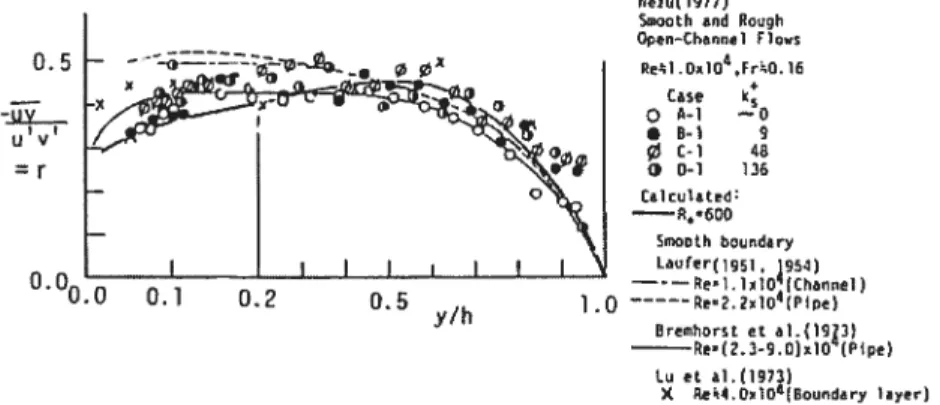
This relatïonship holds over most ofthe depth, 0.05 <z/Z< I for a fully developed

turbulent boundary layer, particularly for high Reynolds numbers, Re [Tennekes and LumÏey, 1972; Nezzt and Nakagmva, 1993; Kironoto and Gra/ 1994]. u, is obtained by extrapolating the linear stress profile to z/Z 0. 1f a vertical stress profile is flot available, u, can be estimated directly from —piZW values obtained

close to the bed. The Reynolds stress extrapolation method of estimating u, has been widely used in flume studies, and in situ environments such as gravel-bed rivers and has been found to give unbiased estimation of u, [Voulgaris and Trowbridge, 199$; Nikora and Goring, 2000; Song and Chiew, 2001; Biron et al., 2004]. In a comparative study of u, estimation methods, Biron et aÏ. [2004] recommended the —piïW extrapolation method for uniforrn flows. In the wake of

LREs and complex flow environments the vertical —piW profile may flot be linear and therefore u, may be estimated from single point near-bed —pïïW observations. Single point estimations do not dependent on z and represent the unbiased estimation of u, [Kim et aÏ., 2000]. The Reynolds stress estimation of u, is susceptible to errors due to improper sensor alignment [Kiti, et aÏ., 2000; Biron et aÏ., 2004] (i.e., if the velocity sensor is not aligned with the longitudinal it

velocity direction, —pïïW estimated values will be contarninated by y component

velocity fluctuations). With 3D velocity measurements, such as obtained with an acoustic Doppler velocimeter (ADV), a rotation of the data is recommended to correct for obvious misalignment [Roy et aÏ., 1996]. In complex 3D flow environments, 2D uniform flow can no longer be assumed and the —pïiW stress

profite deviates from the linear relation of Eqtiation 2.4 [Nezu and Nakagawa, 1993] and rnay underpredict true u, vatues [FapanicoÏaoït andHiÏÏdale, 2002]. In complex flow environments, both vertical momentum flux components —pïW

and —piÎi should therefore be included in u, estimations following Nikora et al.

10

iv) measurements at a single-point near the bed (z = 0.1Z) ofthe 3D turbulent kinetic

energy,ke:

ke= 0.5(1112_{+ V’2+w’2) (2.5)}

u=,fiK _(2.6)

where the prime denotes the root mean square (RMS) values of the instantaneous velocity measurements and C is an cmpirical proportionality constant (c. 0.20) which is assumed to be constant under widely varying conditions [Soulsby, 19831. While this method incorporates thc influence of ail three velocity components, it is dependent on an empirical constant obtained from atmospheric and marine boundary tayers which may flot hold for gravel-bed rivers or complex flows. The IKE mcthod of estimating u. has been shown to give comparable resuits to other estimation rnethods in an annular smooth-bed flctme experiment and in a tidal boundary layer [Thompson et ai, 2003; Kim et aÏ., 2000]. In a mobile sand-bed flume experiment by Bfron et aÏ. [2004], the spatial distribution of’ u. estimates using the TKE mcthod produced the best match with topographic scour hote patterns formed adjacent to flow deflectors. In this complex flow study, the TKE method was found to give more reliable resuits than the Reynolds stress method.

The foregoing discussion has idcntified the theoretical differences between smooth and rough boundary laycrs and discussed some ofthe discrcpancies in applying 2D fully developed boundary layer theory to gravei-bed rivets. The logarithmic velocity profile is iikeiy disrupted by LREs and should not be used to estimate u.. While the TKE method of estimating u shows promises, it has flot been fully tested in gravel-bed rivets with LRE and dtie to its reliance on an empirical constant should be used with caution. Prudence shouid as well be observed whcn using the Reynolds stress method for estimating ii. in the presence of LREs, yet this method bas becn weli tested in gravel

bed rivets and is based on sound boundary layer theory. The following subsection discusses the effect ofincreasing bed roughness on standard turbulence statistics.