Development and validation of a full-time-scale semi-analytical model for the short- and long-term simulation of vertical geothermal bore fields

(1)

Titre:

Title:

model for the short- and long-term simulation of vertical

_{geothermal bore fields}

Auteurs:

Authors: Alex Laferrière, Massimo Cimmino, Damien Picard et Lieve Helsen

Date: 2020

Type:

Article de revue / Journal article

Référence:

Citation:

Laferrière, A., Cimmino, M., Picard, D. & Helsen, L. (2020). Development and

validation of a full-time-scale semi-analytical model for the short- and long-term

simulation of vertical geothermal bore fields. Geothermics, 86, p. 1-11.

doi:

10.1016/j.geothermics.2019.101788

Document en libre accès dans PolyPublie

Open Access document in PolyPublie

URL de PolyPublie:

PolyPublie URL:

https://publications.polymtl.ca/5507/

Version: Version officielle de l'éditeur / Published version

_{Révisé par les pairs / Refereed}

Conditions d’utilisation:

Terms of Use

: CC BY-NC-ND

Document publié chez l’éditeur officiel

Document issued by the official publisher

Titre de la revue:

Journal Title:

Geothermics (vol. 86)

Maison d’édition:

Publisher:

Elsevier

URL officiel:

Official URL:

https://doi.org/10.1016/j.geothermics.2019.101788

Mention légale:

Legal notice:

Ce fichier a été téléchargé à partir de PolyPublie,

le dépôt institutionnel de Polytechnique Montréal

This file has been downloaded from PolyPublie, the institutional repository of Polytechnique Montréal

(2)

Contents lists available atScienceDirect

Geothermics

journal homepage:www.elsevier.com/locate/geothermics

Development and validation of a full-time-scale semi-analytical model for

the short- and long-term simulation of vertical geothermal bore fields

Alex Laferrière

a

_{, Massimo Cimmino}

a,

_{*, Damien Picard}

b

_{, Lieve Helsen}

b,c

a_{Polytechnique Montreal, Department of Mechanical Engineering, Montreal, Canada}

b_{University of Leuven (KU Leuven), Department of Mechanical Engineering, 3001 Leuven, Belgium} c_{EnergyVille, Thor Park 8310, 3600 Genk, Belgium}

A R T I C L E I N F O Keywords:

Ground heat exchangers Vertical geothermal boreholes

g-Function

Thermal resistance and capacitance Load aggregation

Modelica

A B S T R A C T

This paper presents the development and validation of a full-time-scale semi-analytical bore field simulation model. The model allows for the simulation of bore fields comprised of arbitrarily positioned boreholes while accounting for both short-term transient thermal effects within the boreholes and long-term thermal interactions in the bore field. The g-function of the bore field, obtained from the finite line source solution, is corrected to account for the cylindrical geometry of the boreholes and coupled to a thermal resistances and capacitances model of the borehole interior, thereby extending the scope of g-functions to short time scales. Additionally, an improved load aggregation scheme for ground thermal response calculations allows the model to be used with variable simulation time steps. The complete model is validated using a combination of analytical, experimental and field monitored data to verify both its short-term and long-term behaviour. The model is implemented using the Modelica language as part of an implementation in the open-source buildings simulation library IBPSA.

1. Introduction

Ground heat exchangers (GHEs), comprised of vertical geothermal boreholes, are used in ground-source heat pump systems and ground thermal energy storage systems to achieve highly efficient buildings and communities. Their design involves the accurate prediction of the ground temperatures during the operation of the system. The heat transfer process in GHEs evolves over several time and spatial scales (Li and Lai, 2015). At short time scales (i.e. from minutes to hours), the effects of the transit of the fluid through the GHEs and transient heat conduction through the grouting material dominate the heat transfer process. At medium time scales (i.e. from weeks to months), thermal interference between the boreholes becomes significant. At long time scales (i.e. after several years), heat conduction in the ground becomes three-dimensional and boreholes see significant axial temperature variations. A common strategy for the simulation of geothermal heat exchangers is to use separate models to evaluate heat transfer inside and around the boreholes. In this case, the borehole wall acts as an interface between the models.

Heat transfer between the fluid circulating in the U-tubes and the borehole wall can be represented as a delta-circuit of thermal re-sistances. This delta-circuit links the fluid temperature inside the pipes to the steady-state heat transfer rates between each of the pipes and the

borehole and to the steady-state short-circuit heat transfer rates be-tween each pair of pipes. Thermal resistances can be evaluated analy-tically using the multipole method (Claesson and Hellström, 2011) or its line-source approximation (Hellström, 1991), and also numerically using the finite element method (Lamarche et al., 2010). However, these steady-state methods disregard the transit of the fluid through the GHEs and transient heat conduction through the grouting material. According toEskilson (1987), steady-state approximations of the heat transfer inside the GHEs are valid at time scales t > tb, where

=

tb( 5 / )rb2 s is the borehole characteristic time, rbis the borehole radius

and αs is the ground thermal diffusivity. One-dimensional analytical

methods have been proposed to model the short-term temperature variations inside GHEs. In these methods, the GHEs are divided into three regions: a cylinder volume that accounts for the thermal capacity of the fluid and the fluid-to-grout thermal resistance, a hollow cylinder that accounts for the thermal capacity of the grout and its thermal conductivity, and a semi-infinite cylindrical region that accounts for the ground thermal capacity and thermal conductivity. Recent contribu-tions to these one-dimensional methods are presented by Javed and Claesson (2011)andLamarche (2015). A limitation of one-dimensional analytical methods is that the vertical variation of fluid temperatures is neglected. Thermal resistance and capacitance models account for the transient heat transfer inside the GHEs by adding thermal capacitances

https://doi.org/10.1016/j.geothermics.2019.101788

Received 7 October 2018; Received in revised form 14 September 2019; Accepted 18 December 2019

⁎_{Corresponding author.}

E-mail address:massimo.cimmino@polymtl.ca(M. Cimmino).

Geothermics 86 (2020) 101788

Available online 15 January 2020

(3)

to the delta-circuit of thermal resistances (Bauer et al., 2011; Zarrella et al., 2011) to account for the thermal capacity of the grout material. To account for the vertical variation of fluid temperatures, GHEs are discretized vertically and each vertical GHE segment is modelled using its own thermal resistance and capacitance model (Pasquier and Marcotte, 2012).

Early models for the heat transfer between the borehole walls and the ground were based on the analytical infinite line source and cy-lindrical heat source solutions (Ingersoll et al., 1950; Carslaw and Jaeger, 1946). These solutions neglect axial heat conduction in the ground and they are thus only valid at short to medium time scales where heat transfer is mostly horizontal, that is at times t < ts/10,

where ts(= H2/9αs) is the bore field characteristic time (Eskilson, 1987;

Philippe et al., 2009). The concept of g-functions was introduced by

Eskilson (1987). g-Functions, or temperature response factors, are the average borehole wall temperature response to a unit step total heat injection rate in a bore field. They were initially obtained numerically, but analytical methods based on the finite line source solution have since been proposed, first using isoflux line sources that neglect the time and spatial variations of heat injection rates within the bore field (Zeng et al., 2002; Lamarche and Beauchamp, 2007; Claesson and Javed, 2011), then using isothermal line sources that replicate Eskil-son's method (Cimmino et al., 2013; Cimmino and Bernier, 2014; Lazzarotto, 2016; Cimmino, 2015, 2018; Lamarche, 2017). Tempera-ture variations from variable heat extraction rates are obtained from the temporal superposition of the g-function, using load aggregation schemes (Bernier et al., 2004; Liu, 2005; Claesson and Javed, 2012) or other acceleration techniques (Lamarche, 2009; Marcotte and Pasquier, 2008). Line source methods do not account for the cylindrical geometry of the boreholes, and are thus only valid at time scales t > tb. To extend

the validity of g-functions to short time scales, the long-term thermal response can be matched to the short-term thermal response. In this case, a short-time model is used to evaluate the temperature response factor of a borehole and a correction factor is introduced to the

g-function to ensure continuity of the temperature response at an inter-mediate time (Yavuzturk and Spitler, 1999; Claesson and Javed, 2011; Li et al., 2014). This, however, makes the physical and operational characteristics of the borehole part of the g-function definition. It is then not possible to account for the effect of varying fluid flow rates on the short-time response of the GHEs.

Simulation and design tools are most often distributed as standalone applications (e.g. EED (Hellström and Sanner, 1994), GLHEPRO (Spitler, 2000)) or integrated into building simulation software (e.g. eQuest (Hellström, 2006), EnergyPlus (Fisher et al., 2006)). This limits their use to the simulation or design of GHEs based on known ground (or building) loads or to the simulation of the GHEs as part of building energy systems. One exception is the DST model integrated into the TRNSYS environment (Hellström et al., 1996; Klein, 1988). In the DST model, boreholes are assumed to be uniformly placed in a cylindrical ground region. The two-dimensional radial-axial ground temperature variations are calculated from a finite difference method. The fluid temperatures inside the boreholes and the heat fluxes along their length are calculated from an analytical solution. Being integrated into TRNSYS, the DST model is versatile and can be used in the simulation of various systems (e.g. ground-source heat pumps, thermal energy sto-rage for buildings and communities) using other components in TRNSYS. However, it lacks the capability to handle custom bore field configurations with prescribed borehole positions and does not account for the short-time transient heat transfer inside the boreholes. Other GHE models have been implemented in TRNSYS (e.g. (De Rosa et al., 2015; Ruiz-Calvo et al., 2016)), but they rely on pre-generated g-function values.

This paper details the development of a full-time-scale simulation model, improving and extending the model proposed by Picard and Helsen (2014a,b). The simulation model combines a thermal resistance and capacitance method to model the short-term transient heat transfer inside geothermal boreholes and a g-function method to model the long-term ground temperature changes. Improvements are proposed to the

Nomenclature

α thermal diffusivity (m2_/s)

Q¯ aggregated ground load (W)

Δtagg load aggregation time resolution (s)

ΔTb,0 borehole wall temperature change from prior history (K)

ΔTb,q borehole wall temperature change from ongoing heat

transfer (K)

m mass flow rate (kg/s)

κ load aggregation weighting factor (–)

ν aggregation cell aggregation time (s)

ρ density (kg/m3₎

Nu Nusselt number (–)

Pr Prandtl number (–)

Re Reynolds number (–)

C thermal capacitance per unit length (J/m K)

c specific heat capacity (J/kg K)

D borehole buried depth (m)

d distance (m) g g-function (–) H borehole length (m) h local FLS solution (–) k thermal conductivity (W/m K) Nb number of boreholes (–)

Nc number of aggregation cells (–)

nc number of cells per aggregation level (–)

Ns number of bore field total g-function segments (–)

ns number of borehole g-function segments (–) or borehole

vertical discretization segments (–)

Q heat transfer rate (W)

R thermal resistance (m K/W)

r radius, nominal or outer (m)

s FLS integration variable (–)

T temperature (K)

t time (s)

tb borehole characteristic time (s)

tg grout time constant (s)

ts bore field characteristic time (s)

w aggregation cell temporal width (–)

x spacing (m) or x-axis position (m)

y y-axis position (m)

a short-circuit

b borehole or borehole wall

CHS cylindrical heat source

f heat carrier fluid

FLS finite line source

g undisturbed ground (temperature) or grout

i inner

ILS infinite line source

in inlet

k load aggregation event

o outer

out outlet

p pipe

step step response

u borehole origin segment

(4)

calculation of the g-function using the finite line source solution to account for the cylindrical geometry of the boreholes and extend the validity of the calculated g-function to the short time scales of the short-term model. Also, an improved load aggregation algorithm is proposed to allow for variable simulation time steps. The simulation model is implemented in the Modelica language and it is part of the open-source IBPSA project 1 library (IBPSA Project 1, 2018). The model is compa-tible with models from building systems libraries (e.g. (Wetter et al., 2014; Jorissen et al., 2018)).

2. Model

2.1. Structure of the model

The GHE model described in this paper is developed in the Modelica language, which is a free object-oriented language designed for the development of completely modular simulation models for engineering problems expressed as systems of equations. Modelica allows to pre-scribe acausal relationships between variables. As such, there are no strict inputs and outputs to the model: all model variables are computed as long as the boundary conditions are sufficient to solve the system of equations. In this case, the model can use either of the inlet fluid temperature or the heat transfer rate to the fluid to simulate the bore field and evaluate the returning fluid temperature.

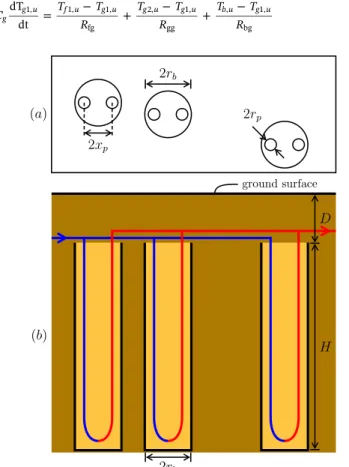
The model simulates one or multiple boreholes positioned in any bore field configuration. Boreholes are vertical, each having one or two U-tubes positioned symmetrically within it. The boreholes are back-filled with grouting material to hold the tubes in place. In the case of double U-tube boreholes, the two U-tubes can be connected either in parallel or in series.Fig. 1shows an example of a bore field containing three arbitrarily positioned single U-tube boreholes. The borehole length H, the buried depth D, the borehole radius rband the pipe

di-mensions (as exemplified by the outer pipe radius rp and the shank

spacing xp) are the same for all three boreholes, as is required by the

model. However, the exact positioning of the boreholes is not limited to any specific geometry (e.g. a grid geometry).

To model the thermal behaviour of the boreholes, it is assumed that the thermal behaviour inside the boreholes can be treated separately from the thermal behaviour between the borehole wall and the sur-rounding soil, each with its own component within the bore field model. This allows for the bore field model to simultaneously account for both the short-term thermal effects (within the boreholes) and the long-term thermal effects (between the boreholes and the surrounding soil).

In the component simulating the heat transfer between the borehole wall and the surrounding soil, the following assumptions are used:

•

The thermal conductivity and the thermal diffusivity of the soil are isotropic, homogenous and constant.

•

The heat transfer is purely conductive.

•

The undisturbed soil temperature far away from the boreholes is uniform along the length of the boreholes.

Regarding the latter assumption, it is possible for this uniform ground temperature to vary over the course of a simulation (e.g. in response to temperature variations at the ground surface), as the ground model evaluates the temperature difference at the borehole wall based on the ground load history and the current heat transfer rate at the borehole wall. As for the borehole model that simulates the heat transfer within the boreholes, the following assumptions are used:

•

The heat capacity and the density of both the grout and the pipes are homogenous and constant.

•

The thermal conductivity of both the grout and the pipes is iso-tropic, homogenous and constant.

•

Axial heat conduction in the grout material and the fluid is

neglected. Heat transfer in the axial direction is purely advective (i.e. due to the fluid flow).

2.2. Borehole model

The role of the borehole model is to describe the heat transfer from the fluid to the borehole wall for a single borehole. Currently, the single U-tube and the double U-tube (connected in parallel or in series) con-figurations are included.

Fig. 2illustrates the structure of the model for a segment of a single U-tube configuration. The borehole is vertically divided into ns

seg-ments of equal length Hu= H/ns. No conductive heat transfer is

mod-elled between the segments and the same borehole wall temperature is applied to each of them. However, energy is still exchanged through advection due to the fluid flow.

The grout and pipes of each borehole segment are modelled by a resistance-capacitance model as proposed by Bauer et al. (2011). It includes two pairs of thermal capacitances (Cgand Cf) for the grout and

the fluid in the case of a single U-tube configuration (four in the case of a double U-tube configuration), two thermal resistances (Rfg) between

the fluid nodes and the grout nodes, a short-circuit thermal resistance between the two grout nodes (Rgg) and two thermal resistances between

the grout nodes and the borehole wall (Rgb). Each tube of each segment

contains a given volume of fluid which is also modelled dynamically. The volume can exchange heat with the pipe by means of convection and with the adjacent fluid volumes by means of advection. The tem-perature of the fluid nodes thus varies with the z-axis (between con-secutive segments). Notice that perfect mixing is assumed when the fluid travels from one segment to the other. Due to this mixing as-sumption, the travel time of the fluid and its effect on the return tem-perature is only approximated by the model. For a borehole segment u, the temperatures of the grout and fluid nodes are given by:

= + + C T T R T T R T T R dT dt g g u1, f u1, g u1, g u g u b u g u fg 2, 1, gg , 1, bg (1a)

Fig. 1. Geothermal borefield with arbitrary borehole positions: (a) top view,

(5)

= + + C T T R T T R T T R dT dt g g u2, f u2, g u2, g u g u b u g u fg 1, 2, gg , 2, bg (1b) = + C T T R m c H T T dT dt ( ) f f u g u f u f f u f u f u 1, 1, 1, fg 1, 1 1, (1c) = + + C T T R m c H T T dT dt ( ) f f u g u f u f f u f u f u 2, 2, 2, fg 2, 1 2, (1d)

wheremf is the fluid mass flow rate.

The convection resistance within each circular pipe is modeled by a constant Nusselt number (Nu) of 3.66 for laminar flows (i.e. when Re ≤ 2300, with Re being the Reynolds number) and by the Dittus–Boelter correlation for turbulent flows (Bergman et al., 2011): Nu = 0.023 Re0.8_Pr0.35_{, where Pr is the Prandtl number. For the} con-duction resistances, the model firstly calculates the fluid-to-ground re-sistance Rband the grout-to-grout resistance Raas defined by Claesson

and Hellström using the multipole method (Claesson and Hellström, 2011). Alternatively, the value of Rbcan be provided, in which case Ra

is calculated from the multipole method and scaled with the fraction between the provided Rb and the Rb computed with the multipole

method. Secondly, Rband Raare used to compute the different

con-duction resistances of the model as prescribed byBauer et al. (2011). The grout capacity values are all identical and their sum corresponds to the thermal capacity of the grout contained in the segment. The loca-tion of the capacities in the grout is also computed according to the method proposed byBauer et al. (2011), except when the computed short-circuit resistance is negative, in which case the capacities are set at the pipe locations.

For the reader's convenience, the equations for the thermal re-sistances and capacities of a single U-tube as described inBauer et al. (2011)are repeated here below. For the double U-tube configuration we refer to their paper:

= +

( )

+ R k k xR 1 Nu ln 2 f d d p g fg p o p i , , (2a) = + R R R xR R R xR 2 ( 2 ) 2 2 g g gg gb ar gb ar (2b) = Rgb (1 x R) g (2c) = C d d c 4 2 g g b p o g 2 , 2 (2d) = C c d 4 f f f p i,2 _(2e)

where kfand kpare the thermal conductivities of the fluid and the pipe,

dp,o and dp,i are the outer and inner diameters of the pipe, db is the

borehole diameter, ρgand cgare the density and heat capacity of the

grout, and ρfand cfare the density and heat capacity of the fluid.

Rg and Rarare respectively the thermal resistance from the pipe

outer wall to the borehole wall and the thermal resistance between the outer wall of the two pipes. They can both be obtained by subtracting the convection and pipe wall resistances from respectively Rband Ra:

= R R k d d k 2 1 Nu ln( / ) 2 g b f p o p i p , , (3a) = + R R k d d k 2 1 Nu ln( / ) 2 a f p o p i p ar , , (3b) Finally, x represents the relative position of the heat capacity Cg

between the pipe outer wall and the borehole wall.Bauer et al. (2011)

propose to locate the heat capacity as follows:

= +

( )

x ln ln d d d d d 2 2 2 b p o p o b p o 2 2_, , , (4)

As the grouting material is modeled with only two heat capacity nodes, Cg, the borehole model's accuracy is limited during fast

tran-sients (e.g. step changes in entering fluid temperature or heat transfer rate). The accuracy of the fluid temperature response is lowered at time scales of the order of the characteristic time tg= Cg· Rb. As will be

shown in Section3.3, acceptable accuracy is obtained at times t > 2tg.

For greater accuracy at times t < 2tg, a higher resolution grout

dis-cretization should be used, such as the disdis-cretization proposed by

Pasquier and Marcotte (2012). 2.3. Ground model

2.3.1. g-Function

The ground temperature response to heat injection is given by the g-function of the bore field. The g-g-function of a bore field represents the borehole wall temperature step-response to constant total heat injection into the bore field, defined by (Eskilson, 1987):

= + T t T Q k g t ( ) 2 HN ( ) b g s b (5)

where Tbis the borehole wall temperature, Tgis the undisturbed ground

temperature, Q is the total heat injection rate into the bore field, ksis

the ground thermal conductivity, H is the borehole length, and Nbis the

number of boreholes. The g-function is configuration specific and varies with the bore field dimensionless parameters; i.e. rb/H the borehole

radius to length ratio, D/H the borehole buried depth to length ratio, and (xi/H, yi/H) the dimensionless positions of the boreholes within the

bore field.

The g-function is calculated using the finite line source solution, following the method ofCimmino and Bernier (2014)and refined by

Cimmino (2018). Each borehole in the bore field is divided into ns

segments of equal length. The bore field is then modelled as a series of Ns (= nsNb) line source segments emitting heat into the semi-infinite

ground region. The total temperature variation at the wall of a borehole segment is obtained by the spatial superposition of the finite line source solution for all line source segments in the bore field:

(6)

= + = T t T Q t k Hh t ( ) ( ) 2 ( ) b u g v N v s u v , 1 , s (6) where Tb,uis the temperature at the wall of a borehole segment u, Qvis

the heat injection rate of a borehole segment v. hu v, is the finite line

source solution for the average temperature change along a segment u caused by heat injection from a segment v, given by (Cimmino and Bernier, 2014): = h t H s d s f s ( ) 1 2 1 exp( ) ( )ds u v u t u v u v , _{1/ 4}_s ₂ 2, 2 , _(7a) = + + + + + + + + + + + + + f s D D H s D D s D D H s D D H H s D D H s D D s D D H s D D H H s ( ) erfint(( ) ) erfint(( ) ) erfint(( ) ) erfint(( ) ) erfint(( ) ) erfint(( ) ) erfint(( ) ) erfint(( ) ) u v u v u u v u v v u v u v u v u u v u v v u v u v , (7b) = = x x x x x

erfint( ) xerf( )dx erf( ) 1 (1 exp( ))

0 2 (7c) = + D D H n u n u n ( 1) floor 1 u s s s (7d)

where Hu(= H/ns) is the length of a borehole segment u, Duis the

buried depth of borehole segment u, αs is the ground thermal

diffu-sivity, and du v, (= (xu xv)2+(yu yv)2) is the distance between

borehole segments u and v. For borehole segments that belong to the same borehole, the finite line source solution in Eq. (7) is evaluated at a distance du v, =0.0005H, rather than at the borehole radius rb. This

distance corresponds to the radius used by Eskilson (1987) for the evaluation of the g-function. Rather than correcting the g-function using the steady-state thermal resistance of a soil annulus, as done byEskilson (1987), the g-function will later be corrected with the cylindrical heat source analytical solution.

Following the definition of the g-function (Eq.(5)), the g-function of the bore field at a time t is obtained by solving Eq.(6)and imposing a constant total heat injection rate into the bore field, a uniform borehole wall temperature equal for all borehole segments and an undisturbed ground temperature of zero:

= = = Q t( ) Q t( ) 2 kHN v N v s b 1 s (8a) = = = T tb( ) Tb,1( )t Tb N, s( )t (8b) = Tg 0 (8c)

This set of conditions correspond to the definition of the g-function as introduced byEskilson (1987).

The g-function evaluated from the finite line source solution is then equal to the uniform borehole wall temperature:

=

gFLS( )t T tb( ) (9)

The spatial superposition of the finite line source solution is illu-strated inFig. 3for the calculation of the influence of a borehole j = 1 on a segment of a borehole i = 3 using ns= 4 segments per borehole.

Note that the superposition of the finite line source solution in Eq.(6)

does not consider the temporal variation of the heat injection rates of the borehole segments. However, as shown by Cimmino (2018), ne-glecting the temporal variation of heat injection rates does not severely impact on the accuracy of the g-function calculation.

As mentioned above, the evaluated g-function needs to be corrected for the cylindrical geometry. Following the work ofLi et al. (2014), the g-function is corrected using the difference of the cylindrical heat source and the infinite line source solutions:

= + = g t( ) g_FLS( )t (g_CHS( )t g_ILS( ,t r 0.0005 ))H _(10a) = + g t s t r J s Y s J s Y s J s Y s s ( ) 2 exp( / ) 1 ( ) ( ) [ ( ) ( ) ( ) ( )] ds s b CHS ₀ 2 2 12 12 0 1 1 0 2 (10b) = g t r E r t ( , ) 1 2 4 s ILS 1 2 (10c) where Jnis the Bessel function of the first kind of order n, Ynis the

Bessel function of the second kind of order n, and E1is the exponential integral. At short time scales, Eq. (10) corrects the g-function to con-sider heat injection from a cylinder instead of from a line source, making the g-function valid for times below tb( 5 / )= rb2 s. At long time

scales, the difference between the cylindrical heat source solution and the infinite line source solution converges to the dimensionless thermal resistance of the ground annulus of inner radius r = 0.0005H and of outer radius r = rb, in agreement with Eskilson's correction factor

(Eskilson, 1987). At short time scales, the finite line source and infinite line source solutions are equivalent and the g-function is then equal to the cylindrical heat source solution.

2.3.2. Load aggregation

The model used to simulate the heat transfer between the ground and the borehole wall uses a modified cell-shifting load aggregation scheme based on that ofClaesson and Javed (2012). A mathematical description of the load aggregation scheme, with proposed improve-ments to allow simulations using variable time steps, is presented in this section.

The thermal load history since the start of heat injection is divided into cells. The number of cells and their width are determined at the start of the simulation. Each cell p has a temporal width wpwhich is

multiplied by the time resolution of the aggregation scheme to de-termine the total length of each cell:

=

wp 2floor(p 1/ )nc (11)

where ncis the number of cells per aggregation level, i.e. the number of

consecutive same-size cells to be reached before cells increase in size. The aggregation time νp(= p 1+ t wagg p) of each cell represents

the extent of past simulation time before the thermal history reaches the following cell:

= = t w p k p k agg 1 (12)

where Δtaggis the time resolution of the load aggregation scheme, which

sets the frequency at which the cell-shifting operation is performed. As a result, lowering its value will generally improve precision while in-creasing computation times.

At a regular interval of Δtagg, the cell-shifting operation is

per-formed. Thermal history is shifted towards more distant cells, while

(7)

ensuring that total aggregated thermal loads are conserved during the shifting operation. For this reason, larger cells will only shift part of their aggregated thermal load. The aggregated loadQ¯p of a given cell

p ≥ 2 is calculated at a discrete aggregation event k according to the values resulting from the previous aggregation event k − 1. Q¯p will

remain null until the current simulation time t is greater than or equal to the aggregation time of the previous cell p − 1, from which point onward cell p will receive shifted thermal history from cell p − 1:

= + < Q w Q Q t ¯pk 1 · ¯ ¯ , p p k pk p p ( ) 1 ( 1) ( 1) 1 (13) When the simulation time then becomes greater than or equal to the aggregation time of cell p, part of the cell's aggregated load will be shifted towards the following cell p + 1:

= + Q w Q w w Q t ¯pk 1 · ¯ 1· ¯ , p p k p p p k p ( ) 1 ( 1) ( 1) (14) The aggregated load of the first cell, which always represents the most recent thermal behaviour, has its value set to the average load over the past Δtagg:

= Q Q t t ¯ k t ( ) dt t 1( ) agg k k 1 (15)

Fig. 4shows an example of the cell-shifting operation being per-formed during a load aggregation event.Fig. 4a shows the values of the aggregated loadsQ¯p(k 1)before the cells are shifted as well as the ground

load since the previous aggregation event tk−1.Fig. 4b then shows the

aggregated loadsQ¯p( )k after being shifted, with the first cell taking the

average ground load over the period from tk−1to tk. This procedure is

then to be repeated at the next aggregation event tk+1; the aggregated

loads will be shifted (fromQ¯p( )k toQ¯p(k+1)) and the first cell will take the

average ground load over the period tkto tk+1as its new value.

To calculate the borehole wall temperature from the aggregated loads, each cell is first given a weighting factor κ. These weighting factors are determined using the bore field's temperature step response Tstep(t), which is calculated with the bore field's g-function g(t). The

weighting factors are thus expressed as: = T t g t k ( ) ( ) 2 HNb s step ₍₁₆₎ = T ( ) T ( ) p step p step p 1 (17)

with Tstep(ν0) = 0. To calculate the borehole wall temperature, the

weighting factors are then used to perform the temporal superposition of aggregated loads. Mathematically, this is the sum of products be-tween κpand the aggregated loadQ¯pof all Nccells:

= = = T tb k( ) T tg k( ) T tb k( ) · ¯Q p N p pk 1 ( ) c (18) Because of the mixing of aggregated loads in the load aggregation scheme, an error is introduced on the resulting averaged loads. However,Claesson and Javed (2012)show that this error is negligible by applying the aggregation scheme over a 20-year simulation with a synthetic load profile.

For the model presented here, the cell-shifting load aggregation scheme of Claesson and Javed (2012)must be adapted to take into account the use of the Modelica language. Two of Modelica's note-worthy features are: (1) the way that system of equations can explicitly use time derivatives of variables (which can be calculated numerically or defined analytically) and (2) the way many Modelica solvers can preemptively determine the moment when a conditional event is trig-gered, at which point an additional simulation time step is created. This means that, regardless of the nominal simulation time step chosen, the actual simulation time steps when using the Modelica language are often variable and can be smaller than the nominal time step. While this

can often be advantageous, as it allows for greater precision and better controllers, it also requires that models are able to handle variable time steps.

The original formulation of the aggregation scheme assumed a constant simulation time step equal to Δtagg. Therefore, the load

ag-gregation scheme has been improved for the present model to account for variable time steps. Starting from the definition of the borehole wall temperature difference as a convolution integral between the loads and time derivative of the thermal response, the temperature change is split in two parts: one representing the contribution from previous load history (i.e. prior to tk−1), and the other representing the contribution

from the ongoing thermal load (i.e. since tk−1):

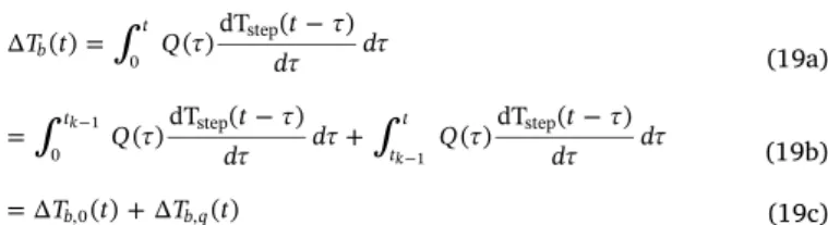
= T t Q t d d ( ) ( )dT ( ) b t 0 step (19a) = Q t + d d Q t d d ( )dT ( ) ( )dT ( ) t t t 0 step step k k 1 1 (19b) = Tb,0( )t + Tb q, ( )t (19c)

Assuming that the current time t is somewhere between two discrete aggregation events such that tk−1≤ t ≤ tk, the first term ΔTb,0(t)

re-presents the temperature difference at the borehole wall caused by the previous load history while assuming no heat injection until the next aggregation event tk. This is calculated by doing the temporal

super-position without the first cell to determine ΔTb,0(tk):

= = Tb ( )tk · ¯Q p N p pk ,0 2 ( ) c (20) Assuming that, in the absence of heat injection, the borehole wall temperature Tb varies linearly in the interval tk−1≤ t ≤ tk, the time

derivative of ΔTb,0can then be expressed explicitly:

= + T t T t T t T t t t t ( ) ( ) ( ) ( )·( ) b,0 b k 1 b,0 k b k 1 k agg 1 (21) = = d T t T t T t T t t ( ) dt ( ) ( ) ( ) b b b k b k ,0 ,0 ,0 1 agg (22)

The second term in Eq.(19c), ΔTb,q(t), adds the contribution of the

heat injection since the last aggregation event. By assuming that the temperature response Tstep(t) varies linearly over a span of 0 ≤ t ≤ Δtagg

(i.e. the interval covered by the first aggregation cell), its time

(8)

derivative since the last aggregation event can be considered constant: = = t T t t t t t dT ( ) dt ( ) , 0

step step agg agg

1

agg agg (23)

This allows for time derivative of ΔTb,q(t) to be expressed as a

function of the current load Q(t): = T t t Q d ( ) · ( ) b q t t , 1 agg k 1 (24) = T t t Q t ( ) · ( ) b q, 1 agg (25)

With both terms in Eq.(19c)expressed as time derivatives, the time derivative of the borehole wall temperature difference can be expressed as follows: = + T tb( ) Tb,0( )t Tb q, ( )t (26a) = T t T t + t t Q t ( ) ( ) · ( ) b,0 k b k 1 agg 1 agg (26b)

This formulation can be directly used in the Modelica language, which allows for systems of equations to use time derivatives of vari-ables with the der() operator.

Fig. 5shows an example of the contribution of both terms in Eq.

(19c)for calculating the borehole wall temperature difference at a si-mulation time step t occuring between two aggregation events tk−1and

tk. 3. Results

3.1. Validation of the load aggregation method

The load aggregation method described in Section2.3.2is validated using the asymmetrical synthetic load profile developed by (Pinel, 2003). This load profile, which uses a constant time step of 1 h with step-wise constant ground loads, is shown for the 20th year inFig. 6a, where positive load values represent heat injection into the ground. The load profile is not synchronized with typical season lengths, which explains why the 20th year shown inFig. 6a is not a full cycle. The validation case is performed on a single U-tube borehole for a simula-tion time of 20 years. The only heat transfer taken into account is that between the borehole wall and the surrounding ground, meaning that the validation case does not include the interior of the borehole. The results are shown inFig. 6. The parameters used for the validation case are shown inTable 1. The resulting borehole wall temperature of the simulated ground model subject to the synthetic load profile is then compared to the exact borehole wall temperature solved in the spectral domain using fast Fourier transforms (Marcotte and Pasquier, 2008). The temperature response factor is the same in both methods and ob-tained using the procedure presented in Section2.3.1.Fig. 6b shows the resulting borehole wall temperature in the 20th year of the simulation model andFig. 6c shows the weekly maximum and minimum deviation in borehole wall temperature between the simulation model and the exact solution (ΔTb,exact− ΔTb,model). The error compared to the exact

solution displays a transient behaviour before reaching a steady peri-odic behaviour after roughly 10 years. The peaks in temperature de-viation coincide with the peaks in heat injection and extraction. The maximum absolute error over the 20-year simulation is 0.083 °C, oc-curring during the third year of the validation case. During the 20th year, the maximum absolute error is 0.077 °C. This error is acceptable and therefore validates the load aggregation method.

3.2. Long-term experimental validation

The ground model (i.e. the combination of the g-function generation procedure and the load aggregation method) is validated

experimentally using the data from the small-scale experiment of

Cimmino and Bernier (2015). In this experiment, heat is injected through a 40 cm long borehole in a sand box of known thermal prop-erties over a period of 1 week (i.e. 168 h). Borehole wall temperatures were measured by thermocouples welded to the borehole wall. Simu-lation parameters are presented inTable 2. Note that the undisturbed ground temperature is not constant throughout the experiment. The sand box is initially at a temperature of 22.09 °C and then increases in temperature due to warm air present at the surface of the sand box.

Cimmino and Bernier (2015)corrected the ground temperature using the analytical solution to conduction in a semi-infinite medium with varying surface temperature. This same correction is used here for the undisturbed ground temperature used in the simulation.

Validation results are shown inFig. 7.Fig. 7a shows the heat in-jection rate during the experiment,Fig. 7b shows the model predicted and measured borehole wall temperature as well as the corrected un-disturbed ground temperature, andFig. 7c shows the error between the predicted and measured borehole wall temperatures. The maximum absolute difference between model predicted and measured borehole wall temperatures is 4.28 °C at a time of 4.15 min. This maximum is observed during the initial start-up phase of the experiment, before the heat injection rate settles to its nominal value of 8.67 W. After the in-itial start-up phase (i.e. for times t > 2.5 h), the maximum absolute difference is down to 0.38 °C at a time of 10.4 h and reaches a maximum value of 1.37 °C at a time of 153.5 h. It should be noted that this ab-solute difference is related to a predicted increase of 42.3 °C above the soil temperature and thus corresponds to 3.2% of the borehole wall temperature change.

3.3. Short-term experimental validation

The short-term behaviour of the bore field model is validated using the sandbox experiment ofBeier et al. (2011). The experiment consists in the injection of heat at an average rate of 1142 W in a 18 m long borehole over a period of 52 h. The measured heat injection rate is used to simulate the inlet and outlet fluid temperature variations using the presented model. The parameters of the experiment are shown in

Table 3. Because the thermal capacity and the density of the filling material were not reported by the authors, their values were instead chosen from the estimated volumetric heat capacity used byPasquier and Marcotte (2014). The construction of the borehole is non-conven-tional: the borehole is contained within an aluminum pipe that acts as the borehole wall. As this modifies the thermal resistances inside the borehole, the Rb value obtained by the thermal response test (TRT)

performed by Beier et al. is used instead of the Rbcomputed by the

multipole method.

Fig. 8 shows that the supply (Tf,in) and the return (Tf,out) fluid

temperatures obtained by the model and by the experiment are in good agreement. A maximum error of 0.76 °C is observed at a time of 1 h, after which the error decreases and reaches a maximum absolute value of 0.33 °C at a time of 36.7 h. The error observed at short times is due to the low resolution of the grout volume discretization, where only two

(9)

thermal capacity nodes are used here to model the grout. At the tem-poral threshold value defined earlier in this paper as 2tg, with tg= CgRb

(=0.93 h, the error is decreased to 0.41 °C and is deemed reasonable for multi-year energy simulations. At times >t 5 /rb2 s (=4.89 h), the root

mean square error is 0.20 °C for both of the inlet and the outlet fluid temperatures.Fig. 9presents the same comparison for the first 5 h of

Fig. 6. Load aggregation method validation: (a) ground loads, (b) simulated

borehole wall temperature, and (c) difference with the FFT predicted borehole wall temperature difference.

Table 1

Parameters used for the load aggregation method validation case.

Parameter Value Units

Borehole length (H) 100 m Borehole buried depth (D) 4 m Borehole radius (rb) 0.05 m

Ground thermal conductivity (ks) 1 W/m K

Ground thermal diffusivity (αs) 1e−6 m/s2

Undisturbed ground temperature (Tg) 0 °C

Load aggregation time resolution (Δtagg) 3600 s

Aggregation cells per level (nc) 5 –

Table 2

Parameters for the long-term experimental validation case.

Borehole length (H) 400 mm Borehole buried depth (D) 19 mm Borehole radius (rb) 6.29 mm

Ground thermal conductivity (ks) 0.262 W/m K

Ground thermal diffusivity (αs) 2.01e−7 m/s2

Fig. 7. Long-term experimental validation: (a) ground load, (b) comparison of

predicted and measured borehole wall temperatures, and (c) error on the pre-dicted borehole wall temperature.

Table 3

Parameters for the short-term experimental validation case.

Parameter Value Units Borehole length (H) 18.3 m Borehole buried depth (D) 0.0 m Borehole radius (rb) 0.063 m

U-tube pipe outer radius (rp) 0.0167 m

U-tube pipe thickness (ep) 0.003 m

U-tube shank spacing (xp) 0.0265 m

Undisturbed ground temperature (Tg) 22.09 °C

Grout thermal conductivity (kg) 0.73 W/m K

Grout volumetric heat capacity (ρgcg) 3.8e6 J/m3-K

U-tube pipe thermal conductivity (kp) 0.39 W/m K

Borehole thermal resistance (Rb) 0.165 m K/W

Fluid mass flow rate (mf) 0.197 kg/s Load aggregation time resolution (Δtagg) 60 s

(10)

the experiment. At this short time scale ( <t 5 /rb2 s), the root mean

square errors are 0.33 and 0.37 °C for the inlet and outlet fluid tem-peratures, respectively.

3.4. Comparison with monitored field data of a Belgian office

The bore field model is validated using measurement data of a 10-year-old medium-size office building located in Dilbeek, Belgium. The building is cooling-dominated and is equipped with a bore field of 37 double-U-tube boreholes of 94 m deep, distributed around the building with a relative distance of 6 m. Two heat pumps of 70 kW each are connected to the bore field as well as heat exchangers for passive cooling. The circulation pump is on/off controlled, creating a maximum flow of 38 m3_/h.

The different bore field parameters are summarized inTable 4. As no TRT has been performed for the building, the thermal conductivity of the ground is retrieved using the SmartGeotherm tool (Geotermische Screeningstool, 2018) and the density and heat capacity of clay is used as the ground is mainly composed of the so-called Ieperiaan Aqui-tardsysteem clay formation. The grout composition comes from the technical sheets of the installation. Finally, a vertical gradiant of 0.01 K/m is assumed.

The validation is performed by comparing the measurement data with the bore field model while imposing the same supply temperature and flow rate. The measurement data of the mass flow are collected by a calorimeter and the inlet and outlet temperatures are measured with Pt100 temperature sensors. The main unknown of the validation is the history of the bore field: the collected measurement data come from a period of seven months of operation after the system had already been running for 10 years. Therefore, the uniform initial ground and grout temperatures of the model had to be tuned to obtain a good fit. Despite the fit, the horizontal temperature gradient in the ground cannot be introduced in the model. Additionally, the calorimeter and the tem-perature sensors are positioned in the cellar. When the pumps are off, the temperatures of the fluid converge to the cellar temperature while this effect is not taken into account by the model. Therefore, the error is only computed when the mass flow is higher than 4 kg/s, and the data is only plotted from that specified threshold.

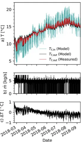
Fig. 10shows the validation results. As expected, a relative large error appears at the beginning of the simulation. This is due to the tuning of the ground and grout temperature: the building is cooling-dominated which means that the ground temperature is increasing over the years. While the undisturbed ground temperature in Dilbeek, Bel-gium, is typically between 10 and 12 °C, the tuning indicates that the average ground temperature is now around 13.5 °C. However, the ground temperature in the neighbourhood of the boreholes is lower as the measurements start in February, at the end of the heating season.

Fig. 8. Short-term experimental validation: (a) ground load, (b) comparison of

predicted and measured temperatures, and (c) error on the predicted fluid temperatures.

Fig. 9. Short-term experimental validation during the first 5 h: (a) ground load,

(b) comparison of predicted and measured temperatures, and (c) error on the predicted fluid temperatures.

Table 4

Parameters for the long-term field validation case.

Borehole length (H) 94 m Borehole buried depth (D) 1 m Borehole radius (rb) 0.075 m

U-tube pipe outer radius (rp) 0.016 m

U-tube pipe thickness (ep) 0.003 m

U-tube shank spacing (xp) 0.0425 m

Undisturbed ground temperature (Tg) 13.5 °C

Initial grout temperature (Tg,0) 9.7 °C

Grout thermal conductivity (kg) 2.35 W/m K

Grout volumetric heat capacity (ρgcg) 1.9e6 J/m3K

U-tube pipe thermal conductivity (kp) 0.42 W/m K

(11)

The error decreases as the effect of the inaccurate ground temperature initialization fades out over time, resulting in an error oscillating be-tween +0.70 and −0.93 °C. A detailed view of the predicted and measured fluid temperatures is shown inFig. 11for a period of 1 week, starting on July 22nd, 2018. It is shown that the short-term changes in the fluid temperatures are adequately reproduced.

4. Discussion and conclusions

This paper presents the development and the validation of a semi-analytical bore field simulation model for short and long time scales. The bore fields are comprised of vertical U-tube boreholes with one or two tubes. A thermal resistance-capacitance delta circuit is used to account for the transient short-term thermal behaviour inside the boreholes. The long-term thermal behaviour within the bore field

(including the interactions between the different boreholes in the bore field) is modelled using the bore field's g-function combined with a cell-shifting load aggregation scheme. The model's range of usability therefore extends from very low time scales (e.g. seconds) to very lengthy ones (e.g. centuries). The ground thermal response model with the proposed load aggregation scheme was validated with a synthetic load profile and showed good agreement with the exact solution. The ground model's long-term behaviour was validated with small-scale experimental data. The complete bore field model was validated using short-term experimental data over the scale of a couple of days and field monitored data from a full-size geothermal field installation over the course of several months. All experimental validation cases showed good agreement between the model's predicted thermal behaviour and the measured data.

The model described in this paper is flexible in regards to bore field parameters, including borehole positions which can be completely ar-bitrary. The properties of the soil, the grout, the pipes and the fluid itself can all be modified independently. The model includes a con-tribution to the finite line source method for g-function calculations which allows it to account for the cylindrical geometry of boreholes. Furthermore, the model includes a contribution to the cell-shifting load aggregation scheme for borehole wall temperature calculations, al-lowing this scheme to be used with variable simulation time steps. The model, developed in the Modelica language, is made freely available to the general public as part of the open-source buildings simulation li-brary IBPSA (IBPSA Project 1, 2018).

Currently, the model is limited to specific borehole geometries, namely vertical (single or double) U-tubes where all boreholes in a given bore field are connected in parallel. Future work will therefore allow the model to simulate bore fields with different borehole con-figurations, including boreholes connected in series, coaxial boreholes, and inclined boreholes. Additionally, future work will include layered surrounding soils with anisotropic properties and groundwater advec-tion.

Conflict of interest

None declared.

Acknowledgements

The authors would like to thank Iago Cupeiro Figueroa for his contribution to the bore field model validation using the measurement data of the Belgian office. The second author acknowledges a start-up subsidy from the Fonds de recherche du Québec – Nature et Technologie (FRQNT) [grant number 2015-B3-181989]. The third and fourth authors acknowledge the funding of their research work by the EUwithin the H2020-EE-2016-RIA-IA programme for the project ‘Model Predictive Control and Innovative System Integration of GEOTABS; –) in Hybrid Low Grade Thermal Energy Systems – Hybrid MPC GEOTABS’

Fig. 10. Comparison with monitored field data of a Belgian office: (a)

com-parison of predicted and measured fluid temperatures, (b) fluid mass flow rate, and (c) error on predicted outlet fluid temperature.

(12)

[grant number 723649 – MPC; GT]. The authors would further like to thank Boydens Engineering, Zedelgem, Belgium for sharing their mea-surement data.

This work emerged from the IBPSA Project 1, an international project conducted under the umbrella of the International Building Performance Simulation Association (IBPSA). Project 1 will develop and demonstrate a BIM/GIS and Modelica Framework for building and community energy system design and operation.

References

Bauer, D., Heidemann, W., Müller-Steinhagen, H., Diersch, H.-J., 2011. Thermal re-sistance and capacity models for borehole heat exchangers. Int. J. Energy Res. 35 (4), 312–320.https://doi.org/10.1002/er.1689.

Beier, R., Smith, M., Spitler, J., 2011. Reference data sets for vertical borehole ground heat exchanger models and thermal response test analysis. Geothermics 40 (1), 79–85.https://doi.org/10.1016/j.geothermics.2010.12.007.

Bergman, T., Incropera, F., DeWitt, D., Lavine, A., 2011. Fundamentals of Heat and Mass Transfer, 7th ed. John Wiley & Sons.

Bernier, M., Pinel, P., Labib, R., Paillot, R., 2004. A multiple load aggregation algorithm for annual hourly simulations of GCHP systems. HVAC&R Res. 10 (4), 471–487.

https://doi.org/10.1080/10789669.2004.10391115.

Carslaw, H., Jaeger, J., 1946. Conduction of Heat in Solids, 2nd ed. Oxford University Press, Oxford.

Cimmino, M., Bernier, M., 2014. A semi-analytical method to generate g-functions for geothermal bore fields. Int. J. Heat Mass Transfer 70 (c, 641–650.https://doi.org/10. 1016/j.ijheatmasstransfer.2013.11.037.

Cimmino, M., Bernier, M., 2015. Experimental determination of the g-functions of a small-scale geothermal borehole. Geothermics 56, 60–71.https://doi.org/10.1016/j. geothermics.2015.03.006.

Cimmino, M., Bernier, M., Adams, F., 2013. A contribution towards the determination of g-functions using the finite line source. Appl. Thermal Eng. 51 (1–2), 401–412.

https://doi.org/10.1016/j.applthermaleng.2012.07.044.

Cimmino, M., 2015. The effects of borehole thermal resistances and fluid flow rate on the g-functions of geothermal bore fields. Int. J. Heat Mass Transfer 91, 1119–1127.

https://doi.org/10.1016/j.ijheatmasstransfer.2015.08.041.

Cimmino, M., 2018. Fast calculation of the g-functions of geothermal borehole fields using similarities in the evaluation of the finite line source solution. J. Build. Perform. Simul.https://doi.org/10.1080/19401493.2017.1423390.

Claesson, J., Hellström, G., 2011. Multipole method to calculate borehole thermal re-sistances in a borehole heat exchanger. HVAC&R Res. 17 (6), 895–911.https://doi. org/10.1080/10789669.2011.609927.

Claesson, J., Javed, S., 2011. An analytical method to calculate borehole fluid tempera-tures for time-scales from minutes to decades. ASHRAE Trans. 117 (2), 279–288.

Claesson, J., Javed, S., 2012. A load-aggregation method to calculate extraction tem-peratures of borehole heat exchangers. ASHRAE Trans. 118 (1), 530–539. De Rosa, M., Ruiz-Calvo, F., Corberán, J., Montagud, C., Tagliafico, L., 2015. A novel

TRNSYS type for short-term borehole heat exchanger simulation: B2G model. Energy Convers. Manag. 100, 347–357.https://doi.org/10.1016/j.enconman.2015.05.021.

Eskilson, P., 1987. Thermal Analysis of Heat Extraction Boreholes (Ph.D. thesis). Lund University, Lund, Sweden.

Fisher, D., Rees, S., Padhmanabhan, S., Murugappan, A., 2006. Implementation and va-lidation of ground-source heat pump system models in an integrated building and system simulation environment. HVAC&R Res. 12 (S1), 693–710.https://doi.org/10. 1080/10789669.2006.10391201.

Geotermische Screeningstool - SmartGeotherm.http://tool.smartgeotherm.be/geo/alg

(Accessed 06 September 2018).

Hellström, G., Sanner, B., 1994. Software for dimensioning of deep boreholes for heat extraction. Proceedings of Calorstock 1994. Espoo/Helsinki, Finland.

Hellström, G., Mazzarella, L., Pahud, D., 1996. Duct Ground Storage Model. Lund – DST. TRSNSYS 13.1 Version January 1996. Tech. Rep. Department of Mathematical Physics, University of Lund, Sweden.

Hellström, G., 1991. Ground Heat Storage: Thermal Analyses of Duct Storage Systems (Ph.D. thesis). Lund University, Lund, Sweden.

X, L., Hellström, G., 2006. Enhancements of an integrated simulation tool for ground-source heat pump system design and energy analysis. In: Proceedings of Ecostock. Pomona NJ, USA.

IBPSA Project 1.https://github.com/ibpsa/modelica-ibpsa(Accessed 19 August 2018).

Ingersoll, L., Adler, F., Plass, H., Ingersoll, A., 1950. Theory of the earth heat exchanger for the heat pump. Heat. Piping Air Condition. 22, 113–122.

Javed, S., Claesson, J., 2011. New analytical and numerical solutions for the short-term analysis of vertical ground exchangers. ASHRAE Trans. 117 (1), 3–12.

Jorissen, F., Reynders, G., Baetens, R., Picard, D., Saelens, D., Helsen, L., 2018. Implementation and verification of the IDEAS building energy simulation library. J. Build. Perform. Simul.https://doi.org/10.1080/19401493.2018.1428361.

Klein, S., 1988. Trnsys – A Transient System Simulation Program. Tech. Rep. University of Wisconsin-Madison, USA.

Lamarche, L., Beauchamp, B., 2007. Short-time analysis of vertical boreholes, new ana-lytic solutions and choice of equivalent radius. Energy Build. 39 (2), 188–198.

https://doi.org/10.1016/j.enbuild.2006.06.003.

Lamarche, L., Kajl, S., Beauchamp, B., 2010. A review of methods to evaluate borehole thermal resistances in geothermal heat-pump systems. Geothermics 39 (2), 187–200.

https://doi.org/10.1016/j.geothermics.2010.03.003.

Lamarche, L., 2009. A fast algorithm for the hourly simulations of ground-source heat pumps using arbitrary response factors. Renew. Energy 34 (10), 2252–2258.https:// doi.org/10.1016/j.renene.2009.02.010.

Lamarche, L., 2015. Short-time analysis of vertical boreholes, new analytic solutions and choice of equivalent radius. Int. J. Heat Mass Transfer 91, 800–807.https://doi.org/ 10.1016/j.ijheatmasstransfer.2015.07.135.

Lamarche, L., 2017. g-function generation using a piecewise-linear profile applied to ground heat exchangers. Int. J. Heat Mass Transfer 115 (B, 354–360.https://doi.org/ 10.1016/j.ijheatmasstransfer.2017.08.051.

Lazzarotto, A., 2016. A methodology for the calculation of response functions for geo-thermal fields with arbitrarily oriented boreholes – Part 1. Renew. Energy 86, 1380–1393.https://doi.org/10.1016/j.renene.2015.09.056.

Li, M., Lai, A., 2015. Review of analytical models for heat transfer by vertical ground heat exchangers (GHEs): a perspective of time and space scales. Appl. Energy 151, 178–191.https://doi.org/10.1016/j.apenergy.2015.04.070.

Li, M., Li, P., V, C., Lai, A., 2014. Full-scale temperature response function (g-function) for heat transfer by borehole ground heat exchangers (GHEs) from sub-hour to decades. Appl. Energy 136, 197–205.https://doi.org/10.1016/j.apenergy.2014.09.013.

Liu, X., 2005. Development and Experimental Validation of Simulation of Hydronic Snow Melting Systems for Bridges (Ph.D. thesis). Oklahoma State University, Stillwater OK, USA.

Marcotte, D., Pasquier, P., 2008. Fast fluid and ground temperature computation for geothermal ground-loop heat exchanger systems. Geothermics 37 (6), 651–665.

Pasquier, P., Marcotte, D., 2012. Short-term simulation of ground heat exchanger with an improved TRCM. Renew. Energy 4, 92–99.https://doi.org/10.1016/j.renene.2012. 03.014.

Pasquier, P., Marcotte, D., 2014. Joint use of quasi-3D response model and spectral method to simulate borehole heat exchanger. Geothermics 51, 281–299.https://doi. org/10.1016/j.geothermics.2014.02.001.

Philippe, M., Bernier, M., Marchio, D., 2009. Validity ranges of three analytical solutions to heat transfer in the vicinity of single boreholes. Geothermics 38 (4), 407–413.

Picard, D., Helsen, L., 2014a. Advanced hybrid model for borefield heat exchanger per-formance evaluation, an implementation in Modelica. In: Proceedings of the 10th International Modelica Conference. Lund, Sweden.

Picard, D., Helsen, L., 2014b. A new hybrid model for borefield heat exchangers perfor-mance evaluation. Proceedings of the American Society of Heating, Vol. 120. Refrigeration and Air Conditioning Engineers, Inc., Seattle, USA.

Pinel, P., 2003. Amélioration, validation et implantation d’un algorithme de calcul pour évaluer le transfert thermique dans les puits verticaux de systèmes de pompes à chaleur géothermiques, Master's thesis. École Polytechnique de Montréal, Montreal, Canada.

Ruiz-Calvo, F., De Rosa, M., Monz, P., Montagud, C., Corberán, J., 2016. Coupling short-term (B2G model) and long-short-term (g-function) models for ground source heat ex-changer simulation in TRNSYS. Application in a real installation. Appl. Thermal Eng. 102, 720–732.https://doi.org/10.1016/j.applthermaleng.2016.03.127.

Spitler, J., 2000. GLHEPRO – a design tool for commercial building ground loop heat exchangers. In: Proceedings of the Fourth International Heat Pumps in Cold Climates Conference. Aylmer, Canada.

Wetter, M., Zuo, W., Nouidui, T., Pang, X., 2014. Modelica buildings library. J. Build. Perform. Simul. 7 (4), 253–270.https://doi.org/10.1080/19401493.2013.765506.

Yavuzturk, C., Spitler, J., 1999. A short time step response factor model for vertical ground loop heat exchangers. ASHRAE Trans. 105 (2), 475–485.

Zarrella, A., Scarpa, M., De Carli, M., 2011. Short time step analysis of vertical ground-coupled heat exchangers: the approach of CaRM. Renew. Energy 36 (9), 2357–2367.

https://doi.org/10.1016/j.renene.2011.01.032.

Zeng, H., Diao, N., Fang, Z., 2002. A finite line-source model for boreholes in geothermal heat exchangers. Heat Transfer Asian Res. 31 (7), 558–567.https://doi.org/10.1002/ htj.10057.