Information Flows in the term structure of commodity prices

Information flows in the term structure of commodity prices

Delphine Lautier∗ Franck Raynaud† March 5, 2014

Preliminary draft

Abstract

Relying on conditional entropy and on the notion of information transfer, we investigate price relationships in the most important commodity futures market: the American crude oil market. We first show that the information shared by futures contracts with different delivery dates increases during the period under scrutiny (i.e. 2000 - 2011). This is especially true for intermediate maturities. When focusing on information transfer, on average on the whole period, it appears that short-term maturities emit more information than long-term ones. This is consistent with the normal functioning of a futures market. A dynamic analysis however reveals that the relative importance of information flows emerging in the far end of the curve (for long-term maturities) arises as integration progresses in the crude oil market. The transmission of shocks from the paper to the physical markets is thus facilitated. Last but not least, the direction of prices moves becomes less stable as time goes on. On the theoretical point of view, these findings raise questions about the segmentation theory and the Samuelson effect.

The authors acknowledge conversations with Michel Robe and fruitful research assistance by G. Boucher and P.A. Reigneron. This article is based upon work supported by the Chair Finance and Sustainable Development and the FIME Research Initiative.

1

Introduction

Financialization is the main concern in commodity markets since a decade. Markets have become more integrated (see for exampleBuyukşahin and Robe(2013) orLautier and Raynaud(2012)); the sustained rise of prices and transactions volume, combined with an intensified presence of investors seeking for diversification through commodity indexes has raised the specter of destabilizing specu-lation. This is especially true for the crude oil market, which is the most important of all. However, no evidence was found that speculation has a destabilizing influence on prices or volatility.

A commodity futures market should fulfill correctly two main economic functions: hedging and price discovery. The hedging function raises the question of the relationships between the physical

∗

DRM-Finance UMR CNRS 7088, Université Paris-Dauphine, Place du Maréchal de Lattre de Tassigny, 75016 Paris. Email: delphine.lautier@dauphine.fr.

†

Lab of Cell Biophysics Ecole Polytechnique Fédérale de Lausanne, Rte de la Sorge, CH-1015 Lausanne. Email: franck.raynaud@epfl.ch

and paper markets. Theoretically, the physical market is the place for the absolute price to appear, as a function of the supply and demand for the underlying asset, whereas the derivative market allows for relative pricing: the futures price derives from the spot price. Under normal circum-stances, the information should flow from the underlying asset to the derivative instrument. This is a central assumption when building term structure models of commodity prices, for example (see among othersSchwartz (1997), which is still a reference nowadays). Is it still true, in the presence of investors taking large positions on the paper market? Is it possible that sudden changes in these positions could induce shocks and create an informational flow spreading from the paper to the physical market?

Price discovery raises another issue, that of the nature of the relationships linking the different maturities together in the derivative market. The informational content of a futures price changes according to the delivery date of the contract. What do the different maturities share and what do they not, especially when considering the short- and long-term parts of the curve? How did this phenomenon evolve through time? Intuitively, we could expect that as time goes on, under the effect of arbitrage operations allowed by rising transaction volumes on all available maturities, the segmentation of the prices curve smoothly disappears. Is is true, now that speculative positions are increasing?

In order to answer these questions, we focus on the futures contracts of the American crude oil market, negotiated on the New York Mercantile Exchange (Nymex). This is indeed the place where the transaction volumes is the highest, worldwide. The crude oil contracts are also characterized by the longer delivery dates (up to 7 years), so the investigation of the term structure is particularly interesting in this case. Our analysis covers a large period of time, from 1998 to 2011. It thus begins before the financiarization process of the commodity markets, generally situated in 2003- 2004. Working on the basis of futures prices we provide, first for an extensive analysis of all maturity link-ages in the crude oil market, second for an investigation of information flows between the different maturities. On that purpose, we rely on the graph theory and on the information theory. The first gives us a way to describe all the prices we are examining, as well as the links between them; the second allows for the study of the informational content of these prices. The first reason underlying the choice of the graph theory is that cross maturity linkages are numerous: there are more than 30 different delivery dates in the crude oil market, that is to say at least 870 pairs of maturities to examine (we actually studied 1740 relationships, as will be explained below). Moreover, such linkages probably change through time, as a result of evolving trading practices. Finally, chances are few that the relationships between different maturities are always linear. So, if we consider that all the futures prices we are studying (ie 30 futures prices per day, during more than 12 years) create a system, then this system is a complex one: it is made of many components, that may interact in various ways through time.

The graph theory precisely deals with complex systems, and provides for very interesting statistical measures in order to examine them. They allow for identifying some recurrent behavior (ie emer-gent rules), to assess the robustness of the empirical findings, and to check for eventual pathological

patterns. A graph (or network) gives a representation of pairwise relationships within a collection of discrete entities. Each point of the graph constitutes a node (or vertex). In this article, a node corresponds to the time series of prices returns of a futures contract. The links (or edges) of the graph can then be used in order to describe the relationships between the nodes. More precisely, the graph can be weighted in order to take into account the intensities and/or the directions of the connections. We do both, on the basis of the information theory.

There are several ways to enrich the information contained in a graph through its links. In finance, for example, the connections between the nodes can be associated to the correlations of price re-turns, or to the positions of the operators. Here, as we are concerned with the information content of the futures contracts, we use the information theory in order to enrich the links of the graph in two ways: first, to determine the intensities of the links; second, to obtain their direction. To the best of our knowledge, such a use is unprecedented in finance.

The theory of information was proposed by Shannon (1948). It aims at quantifying information, which is precisely what we need. Mutual information is a key concept in this context. It gives a precise appreciation of the information (ie uncertainty) shared by two random variables, which are, in our case, the fluctuations of futures prices corresponding to specific delivery dates. Thus the mutual information shared by two futures contracts constitutes the intensities of the links of the graph. At this point, it is interesting to underline that each futures contract might constitute a potential source of information, and / or a potential receiver of information. In order to disentangle between these two possible functions, we introduce some directionality. We rely on conditional entropy: the entropy of our random variable is conditioned by another random variable which is, in our case, the lagged value of another futures contract.

Finally, being able to construct directed graphs gives us the possibility to disclose among futures contracts, between transmitter and receiver and to see how this transmission rule evolves according to time and / or to market conditions.

In what follows, we first expose the methodology used in this paper: it is based on conditional entropy and information transfers. We then present our data and empirical results. Our conclusion proposes theoretical improvements for the modeling of term structure behavior.

2

Methodology

In order to study interdependance and directionality between price movements, we rely on informa-tion theory based on the noinforma-tion of entropy proposed by Shannon (1948). We first present the noinforma-tion of mutual information, which we will use as a proxy for market integration. Within this framework, it is a key concept,that quantifies the dependency between two random variables. Compared to correlations usually used in finance, the mutual information is able to catch non linear relationships between variables. We then expose thow we compute information transfer, that gives a way to study causality relationships.

2.1 Mutual information

Considering a random variable X and its corresponding distribution p(x), the entropy refers to the degree of uncertainty of the variable X and is defined as follows:

H(X) = −X

x

p(x) log p(x), (1)

where P

x is a sum over all the possible states of X.

Considering two variables X and Y with the joint distribution p(x, y), the remaining entropy of X if the values of Y are known is given by the conditional entropy:

H(X|Y ) = −X

x,y

p(x, y) log p(y)

p(x, y) (2)

If the distribution p(x|y) is known, the conditional entropy can be easily rewritten:

H(X|Y ) = −X

x,y

p(x, y) log p(x|y), (3)

and the information between X and Y is: M (X, Y ) =X

x,y

p(x, y) log p(x, y)

p(x)p(y). (4)

It is also possible to expressed the mutual information as:

M (X, Y ) = H(X) − H(X|Y )

= H(X) + (H(Y ) − H(X, Y ))

= H(X, Y ) − H(X|Y ) − H(Y |X),

If the entropies H(X), H(Y ), the conditional entropies H(X|Y ), H(Y |X) and the joint entropies H(X, Y ), H(Y, X) are known, the mutual information can be seen as the reduction of entropy of one variable when the other variables are known.

According to the previous definitions, the mutual information is symmetric if we interchange X and Y . Then M (X, Y ) cannot detect influence of X to Y and vice versa.

2.2 Information transfer

As we aim to identify each futures contract as a potential source or receiver of information, we adopt the formalism proposed by Schreiber (2000) to introduce directionality between futures contracts. Suppose that the value of X at time t + 1 depends on the value of Y at time t. The entropy rate

h1 is defined as:

h1= − X

p(xt+1, xt, yt) log p(xt+1|xt, yt). (5)

Contrary, if X at time t + 1 does not depend on Y at time t, the entropy rate h2 is:

h2 = − X

p(xt+1, xt, yt) log p(xt+1|xt). (6)

Then, the entropy transfer from the variable Y to X is given by the difference between the two aforementionned rates of entropy:

TY →X = h2− h1 = X p(xt+1, xt, yt) log p(xt+1|xt, yt p(xt+1|xt) , (7)

and the transfer from X to Y is:

TX→Y = X p(yt+1, yt, xt) log p(yt+1|yt, xt p(yt+1|yt) . (8)

Using conditional entropies, the two transfers can be rewritten as: TY →X = H(Xt+1|Xt) − H(Xt+1|Xt, Yt)

TX→Y = H(Yt+1|Yt) − H(Yt+1|Yt, Xt)

In the case of a linear dependency between X and Y , for vector auto-regressive processes, the transfer entropy is equivalent to Granger causality. However, it has the major advantage to be model free and to hold in the case of non linearity.

2.3 Measurements

Thanks to this definition of directionality, we are able to build several quantities in order to give evidence of the properties of prices fluctuations in terms of information contents, and to disclose, among futures contracts, between transmitter and receiver:

• the total amount of information send from a maturity • the flow of backward and forward information

• the directionality index

Using Equation (8), we can compute the total amount of information sent from the maturity M to all maturities i:

TMs =< TM →i >i, (9)

and the information received by M :

TMr =< TM ←i >i, (10)

where <>_i denotes the average over all the maturities except M .

We can also compute the flows of forward and backward information to investigate the changes in the direction of information. We use the notion of forward flow to picture information emitted by the short-term maturities, in the direction of long-term maturities; the reverse is true for the backward flows.

The forward flow φ_fis given by:

φf = X X<Y

TX→Y, (11)

and the backward flow φ_b is:

φb = X X>Y

TX→Y. (12)

Finally, to investigate the properties of the directionality between the contracts through the graph theory, we combined Equations (8) and (7) in order to build an index of directionality:

DXY =

TX→Y − TY →X

TX→Y + TY →X

. (13)

DXY gives the strength of the directionality and is bounded by −1 and 1. If DXY is greater than 0

the information flows from X to Y otherwise from Y to X. If we compute DXY for the whole period,

refers as static case, we can obtain the matrix of directionality ¯DXY which represents the static full

directed graph. Computed over time in moving windows, we can get at time t the instantaneous directionality matrix DXY(t) and then we can measure the survival ratio ¯SR(t) as the number of

element of same sign in _N1DXY(t) ∩ ¯DXY.

This quantity reflects the degree of stability of the information in the graph. If ¯SR(t) = 1, the

system has the same flow of information as in the static case, that is to say the market is stable. If ¯

SR(t) = 0, the set of directed links has been completely shuffled indicating disturbances in the flow

of information.

3

Empirical results

In what follows, we first present the data. Then we focus on the information shared by the different contracts, and its evolution through time. We introduce directionality and examine information transfers. Finally we focus on the stability of the transfers.

3.1 Data

The crude oil data are daily settlement prices for the light, sweet, crude oil contract negotiated on the New York Mercantile Exchange (now a division of the Chicago Mercantile Exchange), from 1998 to 2011. When preparing the data, we reconstructed the Nymex calendar in order to determine

0" 20" 40" 60" 80" 100" 120" 140" 160" 5/20/1998"5/20/1999"5/20/2000"5/20/2001"5/20/2002"5/20/2003"5/20/2004"5/20/2005"5/20/2006"5/20/2007"5/20/2008"5/20/2009"5/20/2010" M1" M12" M24"

Figure 1: Crude oil futures prices, Nymex, 1998-2011

precisely which contract has, for example, a one- or a two-month maturity and to determine when the contract changes from the two-months maturity to one-month. We were able to reconstruct 34 time series. The first 28 correspond to monthly maturities (ie from 1 to 28 months). The six last contracts correspond, respectively, to the following maturities : 30, 36, 48, 60, 72 and 84 months. Figure 1 depicts the evolution of these prices on the period under consideration. As can be seen, the prices evolution is characterized by huge rise around 2008, followed by a huge decrease.

Note finally that the analysis below relies on the computation of the price returns of futures prices, ie the daily logarithm price differential ri, with: ri = (ln Fi(t) − ln Fi(t − ∆t)) /∆t, where Fi(t) is

the price of the futures contract with maturity i at t, and ∆t is the time window. Moreover, all dynamic analyses are made on the basis of rolling windows having a length of 500 trading days.

3.2 Mutual information: a proxy for market integration

Let us now examine what happened in this market on the period under consideration, through the lenses of mutual information. Remind that the source of information, in our case, is prices fluctu-ations. Thus, the mutual information depicts the simultaneous dependency or synchronous moves in the prices.

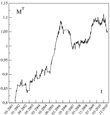
Figure2represents the mutual information shared by all maturities, on the whole period. Thus it depicts the global dynamic behavior of all possible interactions between maturities. The increase in the mutual information provides clear evidence of cross-maturity linkages becoming more and

05-200101-200209-200205-200302-200410-200406-200502-200610-200607-200703-200811-200807-200903-201012-2010

t

M

Figure 2: Mutual information shared by all maturities, 2001-2011

more intense, which can be interpreted as a higher integration of the futures market for crude oil, which is in line with previous studies.

Figure 3gives more insight into this phenomena: it depicts the mutual information per maturity, on the whole period. We can see, again, that the mutual information increases, as the curves of mutual information are getting more and more red as time goes on (going from the front to the back of the picture). What is also evidenced, is that all futures prices do not have the same informational content: the short part of the term structure, which is situated on the left of the picture, contains less mutual information that the long-term part of the curve (on the right). This is consistent with the fact that short-term futures prices are more volatile. Moreover, there is a bulk of mutual infor-mation for middle maturities: the two extremities of the prices curve share less inforinfor-mation with the others than the intermediate one. Such an observation can be attributed to a segmentation of the prices curve into three pieces: from the 1st to the 3rd months, from the 4th to the 27th months, and from the 30rd months to the last delivery date. Finally we can see that as time goes on, the middle part of the curve, where the amount of mutual information is the highest, becomes larger. In other words, the integration phenomenon which can be observed on Figure 3comes mainly from what happens on intermediate maturities.

Figure 4 provides a synthetic view, on the whole period, about the information that a specific maturity shares with all others. It indeed exhibits the average mutual information for each maturity. We can see that the average mutual information is strongly asymmetric. It increases and reaches its maximum near the 18 months maturity. Then it decreases slowly up to the last maturity. Again,

Figure 3: Mutual information per maturity, 2001-2011

!

4!

Lien!avec!le!déport!?!Rien!d’évident.!A!creuser.!

Fig'2b':'évolution'temporelle'de'l’information'mutuelle'par'maturité'sur'le'WTI'(et'sur'le'

Brent,'à'droite)'

!

La! forme! linéaire! du! MST! provient! de! la! forme! en! cloche,! dans! la! figure! 2b.! La!

forme!linéaire!résulte!de!la!structure!des!corrélations,!qui!suit!une!intuition!financière!:!

le!1!mois!est!corrélé!au!2!mois,!lequel!est!corrélé!au!3!mois.!!

Ce!sont!les!maturités!intermédiaires!qui!partagent!la!plus!grande!information!mutuelle!

(là!encore,!c’est!une!conséquence!de!la!structure!des!corrélations).!C’est!un!peu!normal!:!

plus!on!a!de!voisins!qui!partagent!eux!mêmes!de!l’information!avec!d’autres!voisins,!plus!

on!a,!soi!même,!d’information!mutuelle!avec!ces!voisins!(attention!il!n’y!a!pas!de!biais!

dans!le!calcul!qui!défavoriserait!les!deux!extrémités).!!

!

???!Franck,!pourquoi!n’avons!nous!que!8!ans!d’observations!sur!le!WTI!?!!

'

!

!

!

!

Ce!phénomène!de!courbe!en!cloche!est!assez!bien!décrit!par!la!figure!ciVdessous.!!

Figure'2c.'Information'mutuelle'moyenne'par'maturité,'en'statique,'sur'le'WTI'

!

Il!reste!que,!d’une!part,!l’information!mutuelle!moyenne!par!maturité!augmente!dans!le!

temps!(la!surface!est!en!pente!;!ceci!recoupe!la!figure!2a)!et!d’autre!part,!le!nombre!de!

Figure 4: Average mutual information per maturity, 2001-2011

there is more mutual information on the long term part of the curve (up to 7 years) than on the short part (up to 3 months); the explaining factors are not the same for the two sides of the prices curve. Whereas the shortest maturities are mostly influenced by shocks emerging in the physical

market, the behavior of the longest maturities is explained by other factors such as expectations of future supply and demand for the commodity, technological changes, future discoveries, or a lack of liquidity in the futures markets (for more details on these explaining factors, see for example Cortazar and Schwartz (2003)).

3.3 Information flows between maturities

A further step in the analysis of cross-maturity linkages lies in the examination of informational transfers. If we examine the transmission of information between different maturities, the question of which side of the term structure is the transmitter and which one is the receiver is crucial. We first perform a static analysis, on the whole period. We then turn on a analysis of dynamic behaviors.

3.3.1 Static analysis

Figure 5 depicts the informational transfer between maturities recorded on the whole period. The black line corresponds to the information emitted by each maturity, the red one to the information received. The bars represent, for each maturity, the average standard deviation recorded for the measure. They appear to be quite large for the information received on the long-term maturities.

The Figure shows that short-term maturities, up to the 18th months, emit more than they

3.!ANALYSE!DES!TRANSFERTS!D’INFORMATION!

Analyse!des!transferts!d’information,!en!statique!puis!en!dynamique.!!

Transfert!forward!:!des!maturités!les!plus!courtes!vers!les!maturités!les!plus!longues!

Transfert!backward!:!des!maturités!les!plus!longues!vers!les!maturités!les!plus!courtes.!

Quel!signal!influence!quel!signal!?!Pour!nous!le!signal!est!une!fluctuation!de!prix.!!!

3.1.!Analyse!statique!

Figure' 3a':' Information' forward' (en' noir)' et' backward' (en' rouge)' par' maturité':' niveau'

moyen'sur'toute'la'période'

!

Les!barres!d’erreur!représentent!l’erreur,!mesurée!en!moyennant!sur!le!temps.!Chaque!

point!correspond!à!la!valeur!moyenne!du!transfert!d’information!entre!deux!maturités.!

C’est!soit!une!variance,!soit!un!écartVtype!XXX!à!vérifier!par!Franck.!!

Commentaire!:!il!faut!préciser!dans!la!légende!qu’il!y!a!en!plus!les!barres!d’erreur.!Il!faut!

harmoniser!et!parler,!ici!aussi,!d’information!forward!et!backward.!!

Pour!l’information!forward!(en!noir),!on!distingue!trois!segments!de!la!courbe!:!jusqu’à!6!

mois,!entre!6!et!18!mois!et!au!delà.!Entre!1!et!6!mois!l’information!transférée!est!élevée.!

Elle! atteint! un! niveau! maximum! pour! les! maturités! 1! et! 6! mois.! Entre! 7! et! 18! mois!

l’information! transférée! diminue! régulièrement! et! fortement! avec! la! maturité.! Elle!

réaugmente!ensuite,!sur!les!dernières!maturités,!quoique!de!façon!plus!atténuée.!!

On!peut!envisager,!si!requête,!de!calculer!la!distribution!de!l’information!mutuelle!par!

maturités,!mais!alors!on!perdra!le!côté!dynamique!de!l’analyse.!!

Pour! l’info! backward,! il! a! aussi! trois! segments,! mais! positionnés! différemment! en!

fonction! des! maturités!:! entre! 1! et! 10! mois,! l’information! reçue! est! faible,! puis! elle!

augmente!fortement!jusqu’à!environ!20!mois,!puis!elle!augmente!plus!lentement!(pour!

finalement! diminuer.! Les! barres! d’erreurs! sont! beaucoup! plus! écartées! pour! cette!

mesure,!sur!les!maturités!éloignées.!!

Figure 5: Average Information transfer between maturities, 2001-2011

receive. Moreover, most of the information is sent to the very late maturities. The information emitted first increases, till the 6 months maturity, then decreases and finally reaches a plateau. The received information has an inverse tendency: it first decreases, indicating that the short part of the term structure is, on average, less impacted by the flows of information, and then increases, with maximum values at the end of the term structure.

On the theoretical point of view, this analysis shows that market segmentation is not necessarily the same for the information emitted and received.

3.3.2 Dynamical analysis

Let us examine the dynamic pattern of the information transfer, as depicted by Figure6. Here, we do not distinguish anymore between the different maturities: we illustrate what is emitted by all maturities (forward flows) and what is received by all of them (backward flows). To test wether the measurements of forward and backward information flows are statistically significant, we compare them with flows computed from gaussian distributed returns. To do so, we calculate for each time series i in the rolling windows the mean µ_i and the variance σ_i2 and we replace the original datas with surrogate time series drawn from gaussian distribution N (µi, σ2i).

As we can see, dramatic changes can be observed through the period. In the beginning, between

05-2001 09-2002 02-2004 06-2005 10-2006 03-2008 07-2009 12-2010

t

3

4

5

6

7

8

9

10

φ

_info

φ

φ

φ

φ

Figure 6: Information transfer between maturities, 2001-2011

2001 and March 2008, due to market integration, the two flows have a decreasing pattern. Moreover,

the forward flow is higher than the backward one. The relative importance of the former however decreases until the point, in 2008, when the two quantities become somehow equivalent. Thus, whereas in the beginning of the period, the term structure of futures prices was heavily influenced by shocks arising in the short term part of the curve, this is not true anymore after 2008. This mean that the short-term prices (and consequently the physical prices) can be strongly influenced by price fluctuations moving backward in the maturity space. In other words, due to market integration, the driving forces of price movements become equivalent all along the term structure, and may propagate as easily in the forward direction as in the backward one.

3.3.3 Properties of information transfer

Let us finally rely on graph theory to approach the dynamical properties, and more precisely the stability of the information transfers. To do so, we built an oriented graph and we examine its stability (remind that a graph can be defined as a triple, consisting of a nodes set, a links set, and the relation associating nodes with links).

In what follows, we consider a graph where all possible connections are taken into account. More

We then rely on graph theory to approach the dynamical properties, and more

precisely the stability, of the directionality of the information as time goes on.

Among all the possibilities to buid graphs from financial time series (mettre des

ref) we focus on the unweighted directed full connected graph. The links are

oriented according to the matrix of directionality. For a couple X and Y, is the

element of the matrix Txy is greater than Tyx, then the edge is oriented from X to

Y, otherwise from Y to X. Extracted from the directionality matrix computed in the

static case, the corresponding directed graph is presented on Fig 5_1. We clearly

observe that the last maturities (that appear in the center of the graph) are the

nodes where the links point in. This is our state of reference, in the sense that

such an overall directionality shows that the derivative market works well (pas

tres inspiré, mais c est l idee). To get a deeper insight of the market stability, we

calculate the survival ratio which represents at time the fraction of links with the

same orientation at a time t as in the stable state. Before 2008, the survival ratio

displays some variations and fluctuations around a value of 70 %. This result

indicates that most of the links remain in the same state as in the stable state.

After march 2008, the value decreases meanwhile the fluctuations increase as a

result of large changings in the direction of the information flow. Nevertheless, the

system has 2^N possible states, where N is the number of links, and even if

numerous edges switch their direction, nothing says a priori that the new states of

Figure 7: Full connected graph

precisely, the nodes stand for time series of futures price returns, ie one node per maturity. The links are oriented according to the matrix of directionality D_XY, which measure the strength of the information transfer: for a couple of nodes (X,Y), if the element of the matrix TX→Y is greater

than T_{Y →X}, then the edge is oriented from X to Y, otherwise from Y to X.

Extracted from the directionality matrix computed in the static case (on the whole period), the corresponding directed graph is presented on Figure7. We can observe that the last maturities, in the center of the graph, are those where the links point in. In what follows, we consider this graph as a benchmark case, first because it represents what happens on the whole period, second because this configuration correspond to the intuitive way of functioning for a futures markets, where prices shocks are expected to rise in the physical market - here represented by the short-term maturities - and to be transmitted to the paper market.

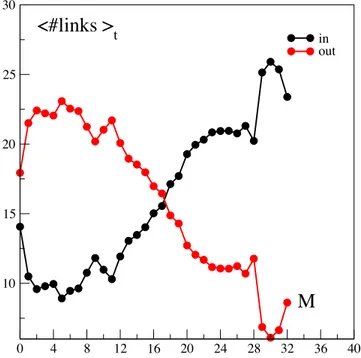
More information is given by a connectivity analysis, like the one depicted by Figure 8. It exhibits

!

21!

Du!point!de!vue!de!la!connectivité,!une!première!question!peut!être!posée!:!y!aVtV

il! des! maturités! critiques,! qui! reçoivent! ou! qui! envoient! plus! d’information! que! les!

autres!?!!

Une!analyse!statique!(sur!toute!la!période)!de!cette!question!donne!les!résultats!

reproduits! sur! la! figure! 4b! (attention,! dans! ce! cas,! on! comptabilise! le! nombre! de! flux!

entrants!ou!sortants,!et!non!la!quantité!d’information!transférée).!!

Figure' 4b.' Somme,' par' maturité,' du' nombre' de' flux' sortants' (out,' ou' forward),' de' flux'

entrants'(in,'ou'backward)';'analyse'statique,'sur'toute'la'période.'

'

La!figure!4ba!ressemble!à!la!figure!3a,!représentant!les!quantités!d’information!forward!

et!backward!transmises!par!maturité!sur!l’ensemble!de!la!période.!Ce!qui!se!produit!du!

point!de!vue!du!nombre!de!flux!entrants!et!sortants!et!cohérent!avec!ce!qui!se!passe!du!

point! de! vue! de! la! quantité! d’information! échangée.! En! revanche,! parce! que! l’on!

s’intéresse! à! un! nombre! de! liens! qui! reste! inchangé,! il! y! a! une! symétrie! entre! liens!

entrants!et!sortants!qui!n’apparaissait!pas!auparavant.!!

Les! maturités! qui! ressortent,! du! point! de! vue! de! la! connectivité! sont,! pour! les! flux!

sortants!:! 6! mois,! 3! mois,! 12! mois,! 36! et! 84! mois.! Si! un! choc! survient! sur! l’une! de! ces!

maturités,! il! affectera! particulièrement! fortement! les! autres! contrats.! Pour! les! flux!

entrants,!ce!sont!les!maturités!1!mois,!!10!mois,!60!mois!qui!sont!le!plus!susceptibles!de!

réceptionner!des!chocs.!!

XXX!Franck,!est!ce!que!l’on!peut!dire!que!le!centre!du!graphe,!du!point!de!vue!des!

flux!sortants,!se!trouve!au!niveau!de!la!maturité!6!mois,!et!du!point!de!vue!des!flux!

entrants,!au!niveau!de!la!maturité!60!mois!?!XXX!!

4.3.! Connectivité! au! sein! du! graphe! complet! dirigé!:! analyse! dynamique! des! flux!

entrants!

M

<#links >

Figure 8: Number of in and out flows, static analysis

the number of links associated to each maturity; up to the 18th months maturity, the links "out" are more numerous than the links "in". Interestingly, the six-month maturity appears to be very important, as it sends a lot of information (far more than the first month maturity). Conversely the deferred maturities are critical because they receive a lot.

To get a deeper insight of the stability properties of the graph, we calculate the survival ratio ¯SR(t).

Remind that if ¯SR(t) = 1 , the system has the same flow of information as in the static case, that

is to say the market is stable. If ¯SR(t) = 0, the set of directed links has been completely shuffled

indicating disturbances in the flow of information.

We can see that before March 2008, the survival ratio displays some variations and fluctuations around a value of 70 percent. This results indicates that most of the links remain in the same state as in the benchmark case. After that date, the value decreases.

05-200101-200209-200205-200302-200410-200406-200502-200610-200607-200703-200811-200807-200903-201012-201008-201104-2012

t

S

(t)

Figure 9: Survival ratios / benchmark case

4

Conclusion

Relying on conditional entropy and on the notion of information transfer, we investigate price re-lationships in the American crude oil futures market. We first show that the information shared by futures contracts with different delivery dates share an increasing amount of information. This is especially true for intermediate maturities. When focusing on information transfer, on average on the whole period, it appears that short-term maturities emit more information than long-term maturities, which is consistent with the normal functioning of a futures market. A dynamic analysis however reveals that price movements can now propagate as easily in the forward direction as in the backward one. Last but not least, the direction of prices becomes less stable as time goes on.

These empirical findings raise theoretical questions. The first concern the segmentation theory. The questioning on the information provided by the term structures of futures prices and the pos-sible presence of a market segmentation dates back to Modigliani and Sutch (1966). Segmentation can be defined as a situation in which different parts of the prices curve are disconnected to each other. On the basis of the informational value of futures prices, Lautier (2005) shows that such a segmentation can be identified on the crude oil futures markets, but that as time goes on, and more precisely as a result of a development process of the market, this phenomenon tends to become less

important. On the basis of a dataset including trader positions, Buyuksahin et al (2009) confirm that the linkages between crude oil futures prices rise with time and show that this is partly due to increased market activity by commodity swap dealers, hedge funds and other financial traders. Buyuksahin et al (2010) then enlarge the question to the informational content of futures prices in the context of management practices using commodity markets as a class of asset. Focusing on futures prices, we complement these works by proposing a way to quantify the information shared by the different futures contracts according to their maturity, and to see how this quantity evolves through time. Finally, we show that the notion of segmentation should make a distinction between forward flows of information and backward flows.

More importantly, the second theoretical question raised by this work is that of the Samuelson effect and calls for a re-appraisal of this effect.

It is common to assert, in the literature on derivative markets (and especially commodity derivative markets), that the behavior of prices is characterized by a difference between the price behavior of first nearby contracts and deferred contracts. The movements in the prices of the prompt contracts are large and erratic, while the prices of long-term contracts are relatively still. This results in a decreasing pattern of volatilities along the price curve. This phenomenon was first explained by

Samuelson(1965). Intuitively, it happens because a shock affecting the nearby contract price has an

impact on succeeding prices that decreases as maturity increases. Indeed, as futures contracts reach their expiration date, they react much more strongly to information shocks, due to the ultimate convergence of futures prices to spot prices upon maturity. These price disturbances influencing mostly the short-term part of the curve are due to the physical market, and to demand and supply shocks.

Despite some debate about statistical measures, this hypothesis has found an large empirical sup-port. Anderson(1985), Milonas (1986) and Fama and French (1987) provided positive results for a large number of commodities and financial assets. More recently, on a theoretical and on an empirical point of view, Deaton and Laroque (1992), Deaton and Laroque (1996), Chambers and

Bailey(1996) showed that the Samuelson effect is a function a storage costs. More precisely, a high

cost of storage leads to relatively little transmission of shocks via inventory across periods. As a result, futures prices volatility declines rapidly with the maturity. Lastly, Fama and French(1988) showed that violations of the Samuelson effect might occur at a shorter horizon when inventory is high. In particular, price volatilities can initially increase with the maturity of the contract, because with enough inventories, stocks-outs may not be possible for the nearest delivery months. Finally,

Bessembinder et al. (1996) show that a mean reverting behavior is necessary for the Samuelson

effect to appear.

In all articles about the Samuelson effect (except maybe that of Anderson and Danthine (1983)), the volatility of futures prices is due to shocks arising in the physical market, which are transmitted to the paper market. The term structure of volatilities decreases because the volatility comes from shocks arising in the physical market, which are transmitted in the paper market. The impact of

these shocks is all the more important that the expiration date of the futures contract approaches. In other words, the natural direction for the propagation of shocks is the forward direction, i.e. from short to long-term maturities, with a progressive absorption as the maturities rise. However, as we have seen it in this paper, as a result of an increasing market integration, prices shocks coming from the long term can spread to the short-term maturities and eventually to the physical market. In other words, it is now possible to have backward propagation of prices shocks, from the far end of the prices curve to the physical market. Such shocks can come from the derivative market itself. In this case the problem could be a lack in the liquidity of long-term contracts or destabilizing spec-ulative activities on this part of the curve. Another source of shocks can also be found in sudden changes in the physical conditions expected in the long run. The expectations of the operators are indeed embedded in the prices of deferred futures contracts. Thus a modification in the long-run expectations, due for example to new discoveries or technological advances in the case of energy commodities, might create a shock in the long-term futures prices.

References

Anderson, R. W. 1985. Some determinants of the Volatility of Futures Prices. The Journal of Futures Markets 3:249–266.

Anderson, R. W. and Danthine, J.-P. 1983. The Time Pattern of Hedging and the Volatility of Futures Prices. Review of Economic Studies 50:249–266.

Bessembinder, H., Coughenour, J. F., Seguin, P. J., and Smeller, M. M. 1996. Is there a term structure of futures volatilities? Reevaluating the Samuelson Hypothesis. The Journal of Derivatives pp. 45–58.

Brennan, M. J. and Schwartz, E. S. 1985. Evaluating Natural Resource Investments. Journal of Business 58:135–157.

Buyukşahin, B. and Robe, M. A. 2013. Speculators, Commodities and Cross-market Linkages. Journal of International Money and Finance .

Chambers, M. J. and Bailey, R. E. 1996. A Theory of Commodity Price Fluctuations. Journal of Political Economy 104:924–957.

Cortazar, G. and Schwartz, E. 2003. Implementing a Stochastic Model for Oil Futures Prices . Energy Economics 25:215–238.

Deaton, A. and Laroque, G. 1992. On the Behaviour of Commodity Prices. Review of Economic Studies 59:1–23.

Deaton, A. and Laroque, G. 1996. Competitive Storage and Commodity Price Dynamics. Journal of Political Economy 104:896–923.

Fama, E. F. and French, K. R. 1987. Commodity Futures Prices: Some Evidence on Forecast Power, Premiums and the Theory of Storage. Journal of Business 60:55–73.

Fama, E. F. and French, K. R. 1988. Business Cycles and the Behavior of Metals Prices. Journal of Finance 43:1075–1093.

Kogan, L., Livdan, D., and Yaron, A. 2009. Oil Futures Prices in a Production Economy with Investment Constraint. The Journal of Finance 3:1345–1375.

Lautier, D. H. and Raynaud, F. 2012. Systemic Risk in Energy Derivative Markets: A Graph-Theory Analysis. Energy Journal 33:217–241.

Milonas, N. T. 1986. Price variability and the maturity effect in futures markets. The Journal of Futures Markets 3:443–460.

Richard, S. F. and Sundaresan, M. 1981. A Continuous Time Equilibrium Model of Forward Prices and Futures Prices in a Multigood Economy. Journal of Financial Economics 9:347–371. Routledge, B. R., Seppi, D. J., and Spatt, C. S. 2000. Equilibrium Forward Curves for

Commodities. Journal of Finance 55:1297–1338.

Samuelson, P. A. 1965. Proof that properly anticipated prices fluctuate randomly. Industrial Management Review 6:41–49.

Schwartz, E. S. 1997. The Stochastic Behavior of Commodity Prices: Implications for Valuation and Hedging. Journal of Finance pp. 923–973.

Tang, K. 2012. Time-varying Long-run Mean of Commodity Prices and the Modeling of Futures Term Structures. Quantitative Finance 2:781–790.