HAL Id: tel-02895919
https://pastel.archives-ouvertes.fr/tel-02895919
Submitted on 10 Jul 2020HAL is a multi-disciplinary open access archive for the deposit and dissemination of sci-entific research documents, whether they are pub-lished or not. The documents may come from teaching and research institutions in France or abroad, or from public or private research centers.
L’archive ouverte pluridisciplinaire HAL, est destinée au dépôt et à la diffusion de documents scientifiques de niveau recherche, publiés ou non, émanant des établissements d’enseignement et de recherche français ou étrangers, des laboratoires publics ou privés.
identification
Lotfi Slim
To cite this version:
Lotfi Slim. Detection of epistasis in genome wide association studies with machine learning methods for therapeutic target identification. Quantitative Methods [q-bio.QM]. Université Paris sciences et lettres, 2020. English. �NNT : 2020UPSLM006�. �tel-02895919�
Préparée à MINES ParisTech
Detection of Epistasis in Genome Wide Association
Studies with Machine Learning Methods for Therapeutic
Target Identification
Détection d’épistasie dans les études d’association
pangénomiques avec des techniques d’apprentissage pour
l’identification de cibles thérapeutiques
Soutenue parLotfi Slim
Le 11 Juin 2020École doctorale no621
Ingénierie des Systèmes,
Matériaux, Mécanique,
En-ergétique
Spécialité
Bio-informatique
Composition du jury :
Chloé-Agathe AZENCOTT
MINES ParisTech Directrice de thèse
Gilles BLANCHARD
Universität Potsdam Président du jury
Rapporteur
Karsten BORGWARDT
ETH Zürich Rapporteur
Clément CHATELAIN
SANOFI R&D Examinateur
Pierre NEUVIAL
CNRS & Institut de
Mathématiques de Toulouse Examinateur
Jean-Philippe VERT
MINES ParisTech & Google Invité
Véronique STOVEN
Abstract i
Abstract
By offering an unprecedented picture of the human genome, genome-wide association studies (GWAS) have been expected to fully explain the genetic background of complex diseases. So far, the results have been mitigated to say the least. This, among other things, can be partially attributed to the adopted statistical methodology, which does not often take into account in-teraction between genetic variants, or epistasis. The detection of epistasis through statistical models presents several challenges for which we develop in this thesis a pair of adequate tools. The first tool, epiGWAS, uses causal inference to detect epistatic interactions between a target SNP and the rest of the genome. The second tool, kernelPSI, instead uses kernel methods to model epistasis between nearby single-nucleotide polymorphisms (SNPs). It also leverages post-selection inference to jointly perform SNP-level selection and gene-level significance testing. The developed tools are – to the best of our knowledge – the first to extend powerful statistical learning frameworks such as causal inference and nonlinear post-selection inference to GWAS. In addition to the methodological contributions, a special emphasis was placed on biological interpretation to validate our findings in multiple sclerosis and body-mass index variations.
Résumé iii
Résumé
En offrant une image sans précédent du génome humain, les études d’association pangénomiques (GWAS) expliqueraient pleinement le contexte génétique des maladies complexes. A ce jour, les résultats ont été pour le moins mitigés. Cela peut être partiellement attribué à la méthodologie statistique adoptée, qui ne prend pas souvent en compte l’interaction entre les variants génétiques,
ou l’épistasie. La détection d’épistasie à travers des modèles statistiques
présente plusieurs défis pour lesquels nous développons dans cette thèse une paire d’outils adéquats. Le premier outil, epiGWAS, utilise l’inférence causale pour détecter les interactions épistatiques entre un SNP cible et le reste du génome. Le deuxième outil, kernelPSI, utilise à la place des méthodes à noy-aux pour modéliser l’épistasie entre plusieurs polymorphismes mononucléo-tidiques (SNPs) voisins. Il tire également partie de l’inférence post-sélection pour effectuer conjointement une sélection au niveau des SNPs et des tests de signification au niveau des gènes. Les outils développés sont - au meilleur de nos connaissances - les premiers à étendre au domains des GWAS des outils puissants d’apprentissage statistique tels que l’inférence causale et l’inférence post-sélection nonlinéaire. En plus des contributions méthodologiques, un accent particulier a été mis sur l’interprétation biologique pour valider nos résultats dans la sclérose en plaques et les variations d’indice de masse cor-porelle.
Acknowledgments v
Acknowledgments
I would like to start by thanking Chloé-Agathe Azencott for being a sup-portive advisor and an enthusiastic researcher. Her unique expertise in GWAS helped me navigate the intricacies of the field. Her upbeat attitude has always made our discussions cheerful, even during difficult times. We couldn’t help but joke sometimes about the future of GWAS, but other times, we concluded it was the way to go for bioinformatics and biomedical data science.
The second acknowledgement goes naturally for my second advisor, Clé-ment Chatelain who has taught me a lot about biology and bioinformatics. His input was always valuable and was key to taking our work to the next level. I would also like to thank him for putting up with my whims and caprices.
My thesis director during the first half of my PhD was Jean-Philippe Vert. He is a careful listener and a demanding researcher. Both traits are key for success in academia. My third acknowledgement goes to him for helping me pushing the envelope.
Last but not least among my supervisors is Véronique Stoven. Not only was she incredibly helpful, but also a pleasant and agreeable person to speak to. I have always admired her energy and general culture.
I had the pleasure to collaborate with Hélène de Foucauld from Sanofi. She is a passionate biologist. By contrast, I consider myself a passionate statistician. Combining our respective fields was instrumental in making our work exhaustive and unique.
A PhD can not be successful without supportive lab mates. In that respect, I was incredibly lucky by being a member of the CBIO family. Our research topics are often diametrically opposed, but we always acted like a single and tight-knit group. I will miss our lunches at the Curie canteen and our CBIO meetings. I shared wonderful moments with the PhD candidates of my cohort, Hector and Joe.
As a CIFRE PhD candidate, I also had the pleasure of belonging to a second family, the SANOFI family. They taught me a lot about the corporate life and many topics I was completely ignorant of. I will always remember our nerdiest jokes. It was a strong dose of dark humor that only the strongest can withstand.
I am also indebted to all my friends in particular Ayoub, Olivier, Rafik, Mike and François who were curious and attentive to my research. PhDs are a difficult journey that can become pleasant in the presence of such sympathetic and encouraging friends.
My last and most important acknowledgment goes to my family, my father Aissa, my mother Beya and my sister Lobna. My studies have always been the first priority of my parents. They have made many sacrifices to guarantee
Contents
Abstract i Résumé iii Acknowledgments v List of Figures xi List of Tables xv List of Symbols 1 1 Introduction 11.1 Genome-wide association studies . . . 3
1.2 Missing heritability and epistasis . . . 6
1.3 Understanding the biology of epistasis . . . 8
1.3.1 Intragenic epistasis . . . 8
1.3.2 Intergenic epistasis . . . 9
1.4 Challenges of statistical epistasis . . . 9
1.4.1 Relation to biological epistasis . . . 10
1.4.2 The definition of interaction . . . 10
1.4.3 Population structure . . . 12
1.4.4 Linkage disequilibrium . . . 13
1.4.5 High dimensionality . . . 13
1.4.6 Nonlinearity. . . 14
1.4.7 Hypothesis testing . . . 15
1.5 Bridging the gap with statistics . . . 16
1.5.1 epiGWAS . . . 17
1.5.2 kernelPSI . . . 17
1.6 Bridging the gap with biology . . . 19
1.6.1 Multiple sclerosis . . . 19
1.6.2 Variations of BMI . . . 19
1.7 Contributions . . . 20
2 EpiGWAS: Novel Methods for Epistasis Detection in Genome-Wide Association Studies 21 2.1 Introduction. . . 23
2.2 Material and Methods . . . 25
2.2.1 Setting and notations . . . 25
2.2.2 Modified outcome regression . . . 26
2.2.5 Support estimation . . . 31
2.3 Results. . . 32
2.3.1 Simulations . . . 32
2.3.2 Case study : type II diabetes dataset of the WTCCC . . . . 36
2.4 Discussion . . . 39
3 kernelPSI: a Post-Selection Inference Framework for Nonlinear Variable Selection 43 3.1 Introduction. . . 45
3.2 Settings and Notations . . . 46
3.3 Kernel Association Score. . . 46
3.4 Kernel Selection . . . 48 3.5 Statistical Inference . . . 50 3.6 Constrained Sampling . . . 52 3.7 Experiments. . . 53 3.7.1 Statistical Validity . . . 53 3.7.2 Benchmarking . . . 54
3.7.3 Case Study: Selecting Genes in a Genome-Wide Association Study . . . 57
3.8 Conclusion . . . 59
4 A systematic analysis of gene-gene epistasis in multiple sclerosis pathways 61 4.1 Introduction. . . 63
4.2 epiGWAS: from the SNP level to the gene level . . . 64
4.2.1 Detecting SNP-SNP synergies with epiGWAS . . . 64
4.2.2 Gene-level epiGWAS . . . 64
4.3 Data and experiments . . . 65
4.3.1 Genotypic data . . . 65
4.3.2 Variant selection . . . 66
4.4 Results. . . 68
4.4.1 Enrichment analysis for obtained subnetworks. . . 70
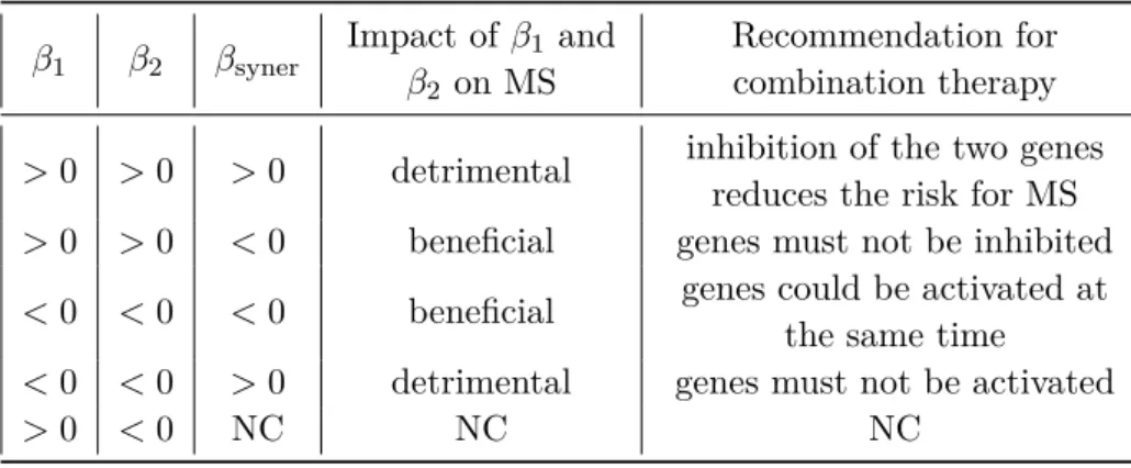
4.4.2 Directionality of the synergy . . . 70
4.4.3 Biological interpretation . . . 72
4.5 Conclusion . . . 77
5 Nonlinear post-selection inference for genome-wide association stud-ies 79 5.1 Introduction. . . 80
5.2 KernelPSI: post-selection inference for big genomic data . . . 81
5.2.1 Outcome normalization . . . 82
5.2.2 Contiguous hierarchical clustering for genomic regions . . . . 83
Contents ix
5.2.4 Efficient nonlinear post-selection inference for high-dimensional
data . . . 84
5.3 A study of BMI and its variation in the UK BioBank. . . 86
5.3.1 Data and experiments . . . 87
5.3.2 Results . . . 89
5.4 Conclusion . . . 93
6 Conclusion and Perspectives 95 A EpiGWAS supplementary material 101 A.1 Genotypic hidden Markov model . . . 101
A.2 Additional simulation results for epiGWAS . . . 103
A.2.1 First scenario: synergistic only effects . . . 103
A.2.2 Second scenario: partial overlap between marginal and syn-ergistic effects. . . 105
A.2.3 Third scenario: partial overlap between quadratic and syner-gistic effects . . . 107
A.2.4 Fourth scenario: partial overlap between quadratic/marginal and synergistic effects . . . 109
B KernelPSI supplementary material 111 B.1 Proof of Lemma 3.1 . . . 111
B.2 Proof of Theorem 3.1. . . 114
B.3 Additional experiments on kernelPSI . . . 116
B.3.1 Statistical validity: Statistical power of kernelPSI for different effect sizes, on simulated data . . . 116
B.3.2 Benchmarking for the first configuration: using Gaussian ker-nels over simulated Gaussian data . . . 117
B.3.3 Benchmarking for the second configuration: using linear ker-nels over simulated binary data . . . 119
B.3.4 Benchmarking for the third configuration: using Gaussian kernels over simulated Swiss roll data . . . 121
B.3.5 Kernel selection performance . . . 124
B.3.6 A. thaliana case study of kernelPSI: data description and pre-processing . . . 125
B.3.7 A. thaliana case study: rank concordance between the methods126 B.3.8 A. thaliana case study: list of significant genes . . . 128
B.3.9 A. thaliana case study: non-metric multi-dimensional scaling of the results. . . 129
C EpiGWAS on multiple sclerosis: supplementary materials 131 C.1 Distribution of SNPs in MS disease maps . . . 131
C.2 Visualization of epiGWAS results on MetaCore disease maps for mul-tiple sclerosis . . . 132
C.4 Content of epiGWAS-selected subnetworks in therapeutic targets . . 143
C.5 MetaCore disease maps for multiple sclerosis . . . 144
C.5.1 Disease map 3305. . . 144
C.5.2 Disease map 4455. . . 145
C.5.3 Disease map 5199. . . 146
C.6 Filtering pipeline . . . 147
C.7 Physical mapping of SNPs selected by epiGWAS . . . 148
C.8 eQTL mapping . . . 149
List of Figures
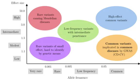
1.1 Impact of variants by risk allele frequency and effect size. In par-ticular, GWAS focus on common diseases caused by a large set of
common variants (bottom-right). . . 4
1.2 Illustration of a GeneChip Human Mapping 500K Array manufac-tured by Affymetrix. The array interrogates SNPs located on
am-plicons that range in size from 200 bp to 1, 000 bp (Komura et al.,
2006). . . 5
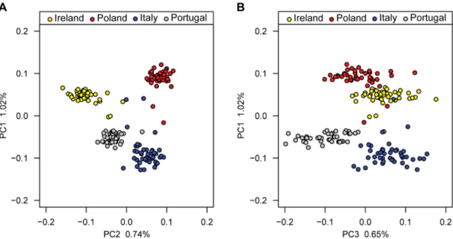
1.3 Example of PCA results showing how GWAS participants can clus-ter by country of origin. PC1 is related to the position along the north-south axis, while PC2 to the position along the east-west axis.
The figure is sourced from Candille et al. (2012) under a Creative
Commons Attribution 2.5 Generic license. . . 12
1.4 Illustration of a Manhattan plot with one significant locus.. . . 15
2.1 Scoring of two SNPs X1 and X2. The scores are the areas under the
first half of their stability paths comprised between λ1 and λ100. . . 32
2.2 Average ROC (left) and PR (right) curves for the fourth scenario and
n= 500 . . . 35
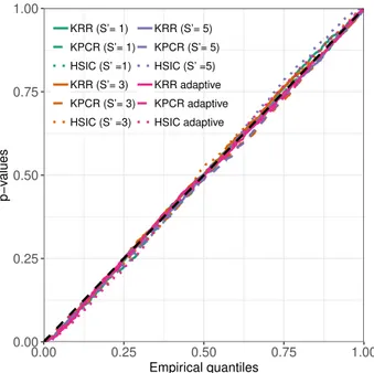
3.1 Q-Q plot comparing the empirical kernelPSI p-values distributions
under the null hypothesis (θ = 0.0) to the uniform distribution. . . . 55
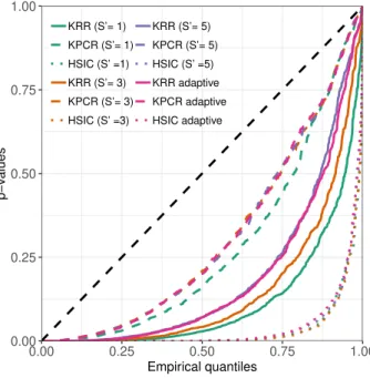
3.2 Q-Q plot comparing the empirical kernelPSI p-values distributions
under the alternative hypothesis (θ = 0.3) to the uniform distribution. 56
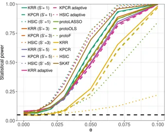
3.3 Statistical power of kernelPSI variants and benchmark methods,
us-ing Gaussian kernels for simulated Gaussian data. . . 56
3.4 Statistical power of kernelPSI variants and benchmark methods,
us-ing linear kernels for simulated binary data. . . 57
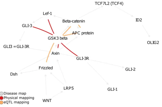
4.1 The 2% top-scoring pairs in DM 3306 for eQTL and physical mappings. 68
4.2 The different types of links between proteins/proteins or
proteins-phenotypes in MetaCore maps . . . 73
4.3 Schematic representation of the role played by the gene pairs
NF-κB/IP10 in the development of demyelination in MS. . . 75
5.1 Clustering methodology: adjacent hierarchical clustering coupled with
the gap statistic to determine the appropriate number of clusters. . . 83
5.2 Comparison of the Beta densities for different values of the shape
parameters (α, β). . . . 85
5.3 A GPU-accelerated pipeline for the evaluation of quadratic constraints. 86
5.4 Comparison of the empirical c.d.fs of BMI and ∆BMI to the c.d.f of
neighbor among the SNPs in the clusters selected by kernelPSI. . . . 90
5.6 A violin plot comparing the p-values of kernelPSI for BMI and ∆BMI
to two benchmarks.. . . 92
A.1 Average ROC (left column) and PR (right column) curves for the
first scenario . . . 103
A.2 Average ROC (left column) and PR (right column) curves for the
second scenario . . . 105
A.3 Average ROC (left column) and PR (right column) curves for the
third scenario . . . 107
A.4 Average ROC (left column) and PR (right column) curves for the
fourth scenario . . . 109
B.1 Q-Q plots comparing the empirical kernelPSI p-values distributions under the alternative hypothesis to the uniform distribution, for
dif-ferent effect sizes θ. The data is generated as described in Section 3.7.1.116
B.2 Q-Q plots comparing the empirical kernelPSI and benchmarking p-values distributions under the null (θ = 0) or alternative hypothesis (θ > 0) to the uniform distribution, for different effect sizes θ, using Gaussian kernels for simulated Gaussian data. The data generation
and benchmarked methods are described in Section 3.7.2. . . 118
B.4 Q-Q plots comparing the empirical kernelPSI and benchmarking p-values distributions under the null (θ = 0) or alternative hypothesis (θ > 0) to the uniform distribution, for different effect sizes θ, using linear kernels for simulated binary data. The data generation and
benchmarked methods are described in Section 3.7.2. . . 120
B.5 Q-Q plots comparing the empirical kernelPSI and benchmarking p-values distributions under the null (θ = 0) or alternative hypothesis (θ > 0) to the uniform distribution, for different effect sizes θ, using Gaussian kernels for simulated Swiss roll data. The data generation
and benchmarked methods are described in Section 3.7.2. . . 122
B.6 Statistical power of kernelPSI variants and benchmark methods,
us-ing Gaussian kernels for simulated Swiss roll data. . . 123
B.7 Non-metric multi-dimensional scaling (NMDS) of the p-values ob-tained by the kernelPSI and benchmark methods on Arabidopsis
thaliana data, using 1 − τ as a distance. . . . 129
C.1 figure . . . 141
C.2 Sonic Hedgehog signaling in oligodendrocyte precursor cells
differen-tiation in multiple sclerosis (DM 3305). . . 144
C.3 Inhibition of remyelination in multiple sclerosis: regulation of
List of Figures xiii
C.4 Cooperative action of IFN-gamma and TNF-alpha on astrocytes in
multiple sclerosis (DM 5199). . . 146
List of Tables
1.1 Estimation of missing heritability for several complex diseases . . . . 7
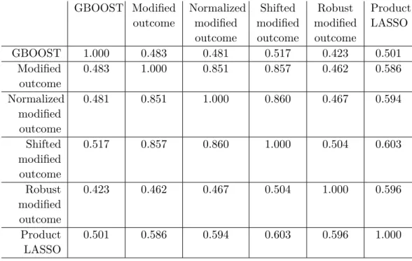
2.1 Concordance between methods used to determine SNPs synergistic to rs41475248 in type II diabetes, measured by Kendall’s tau. . . . 38
2.2 Concordance between methods used to determine SNPs synergistic to rs41475248 in type II diabetes, measured by Kendall’s tau with multiplicative weights. . . 38
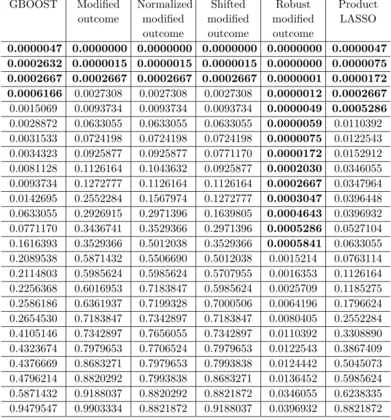
2.3 Cochran-Armitage test p-values for the top 25 SNPs for each method 39 3.1 Ability of the kernel selection procedure to recover the true causal kernels, using Gaussian kernels over simulated Gaussian data. . . 58
4.1 Titles and internal IDs of MetaCore disease maps related to MS. . . 67
4.2 Analysis of the impact of genes up-regulation on the risk for humans to develop MS, for each gene individually (signs of β1 and β2), and for the pair of genes synergistically (sign of βsyner) which is epistasis. 73 5.1 Distribution of the number of selected clusters S0 depending on the total number of clusters S and the phenotype.. . . 91
5.2 Concordance between BMI and ∆BMI by method, according to three Kendall rank correlation measures (standard, multiplicative, additive). 91 A.1 Average ROC and PR AUCs for the first scenario . . . 104
A.2 Average ROC and PR AUCs for the second scenario . . . 106
A.3 Average ROC and PR AUCs for the third scenario . . . 108
A.4 Average ROC and PR AUCs for the fourth scenario . . . 110
B.1 Ability of the kernel selection procedure to recover the true causal kernels, using linear kernels over with binary data. . . 124
B.2 Ability of the kernel selection procedure to recover the true causal kernels, using Gaussian kernels over simulated Swiss roll data.. . . . 124
B.3 Concordance between kernelPSI and benchmark methods, measured by the Kendall’s tau coefficient between the p-values returned for the 50% smallest genes.. . . 126
B.4 Concordance between kernelPSI and benchmark methods, measured by the Kendall’s tau coefficient between the p-values returned for the 50% largest genes. . . 127
B.5 Genes detected as significantly associated to the FT GH phenotype, by method. . . 128
C.1 SNP and gene distributions in each disease map for eQTL and phys-ical mappings . . . 131
edness, complementarity, centrality and commonality. . . 142
C.3 Number of drug targets in the resulting subnetworks for each disease
map and its statistical significance. . . 143
C.4 Pairs of genes identified by physical mapping, and selected on the
basis of their SNPs’ consequence as a protein dysfunction. . . 148
C.5 Compiled results of gene pairs identified by epistasis, and filtered according to the scheme in Fig 4.2, with their specified or unknown
Chapter 1
Introduction
Abstract: Genome-wide association studies have become an
ubiquitous approach to unravel the genetic background of complex diseases. Nonetheless, this background remains largely unexplained. Several hypotheses have already been advanced to explain this missing heritability. One of them is the interaction between distinct loci, or epistasis. Intragenic epistasis and intergenic epistasis are the two major types of epistasis. The detection of both types is subject to several statistical challenges due to linkage
disequilibrium, high dimensionality and population structure, among others. To tackle them, we propose a pair of novel approaches. They help bridge the gap with statistical learning frameworks such as causal inference and nonlinear post-selection inference to improve the detection of epistatic interactions. These tools are further applied to comprehensive use cases to bridge another gap, namely the gap with biology. Specifically, we focus on intragenic epistasis in body mass index and its variations, and on intergenic epistasis in multiple sclerosis. Bridging the two gaps provides an end-to-end pipeline for the study of epistasis. This is often a major shortcoming of epistasis studies, which makes the work conducted in this thesis a significant contribution to the field.
Résumé : Les études d’association à l’échelle du génome sont
devenues une approche essentielle pour démêler le fond génétique des maladies complexes. Néanmoins, ce fond génétique reste largement inexpliqué. Plusieurs hypothèses ont déjà été avancées pour expliquer cette héritabilité manquante. L’un d’eux est l’interaction entre des loci distincts, ou épistasie. L’épistasie intragénique et l’épistase intergénique sont les deux principaux types d’épistasie. La détection des deux types est soumise à plusieurs défis statistiques en raison du déséquilibre de liaison, de la haute dimensionnalité et de la structure de la population, entre autres. Pour y faire face, nous proposons deux nouvelles approches. Ils aident à combler l’écart avec les cadres d’apprentissage
statistique tels que l’inférence causale et l’inférence post-sélection nonlinéaire pour améliorer la détection des interactions
avec la biologie. Plus précisément, nous nous concentrons sur l’épistase intragénique dans l’indice de masse corporelle et ses variations, et sur l’épistase intergénique dans la sclérose en plaques. Combler les deux lacunes fournit un outil de bout en bout pour l’étude de l’épistasie. Il s’agit souvent d’une lacune majeure des études sur l’épistasie, ce qui fait des travaux menés dans cette thèse une contribution significative au domaine.
1.1. Genome-wide association studies 3
1.1
Genome-wide association studies
The human genome project (Risch & Merikangas, 1996) was hailed as a turning point for humanity. It was the first effort to successfully construct a reference genome. Nonetheless, other equally important goals such as determining the bases of genetic diseases remained unattainable. The first steps in this direction were made thanks to Genome-Wide Association Studies, or GWAS (Visscher et al.,2012). These studies rely on datasets comprising the genotypes of numerous participants and their phenotypic measurements e.g. a disease status or a quantitative trait. The statistical association between all genotyped variants and the phenotype is then evaluated. The main rationale is that the discovery of causal variants will further our understanding of biological questions, and hopefully help develop better therapies (Nelson et al.,2015).
Single-nucleotide polymorphisms (SNPs) are the genetic variants of choice in GWAS. They correspond to the substitution of a single nucleotide, the elementary building block of chromosomes. More precisely, SNPs refer to single-nucleotide variants with a frequency larger than 1%. This threshold is owed to the focus of GWAS on common diseases. Behind this lies the hypothesis that common dis-eases are caused by a large set of interacting variants with small effect sizes. This hypothesis is commonly known as the common disease-common variant (CD-CV) hypothesis (see Figure1.1). The other category of single-nucleotide variants – those with a frequency lower than 1% – are referred to as rare variants. They are also the subject of genetic studies, in particular for Mendelian diseases (Pritchard, 2002). Genetic studies can additionally include other types of variants such as copy number variations (CNVs) (Marshall et al.,2016).
SNPs approximately occur at a rate of one in every 300 base pairs (Nelson,2004). 90% of SNPs are located in non-coding regions. The remaining 10% are located in coding regions and can be split into two categories: synonymous (silent) SNPs and nonsynonymous SNPs. Silent SNPs do not alter the amino acid composition of the protein. On the other hand, nonsynonymous SNPs can alter the composition of the protein product in two different ways. If the coding SNP is missense, a complete protein with a different amino acid composition is obtained. Conversely, nonsense coding SNPs often result in incomplete and nonfunctional proteins.
SNPs located in non-coding regions can have an impact in several ways. For instance, they may influence promoter activity (gene expression), messenger RNA (mRNA), conformation (stability), and translational efficiency (Shastry,2009).
In GWAS, genotypes are typically encoded as the number of allelic mutations at every measured SNP. For biallelic SNPs, this is equivalent to an encoding in {0, 1, 2}. The positions of the measured SNPs depend on the genotyping technology. In GWAS, the most common technology are SNP arrays thanks to their low cost and high accuracy. Probe-based arrays can now genotype an individual with a > 99% accuracy (LaFramboise,2009) for less than 250 dollars 1. We give an illustration
1
Allele frequency
Very rare Rare Low frequency Common
High
Intermediate
Modest
Low
Rare variants of small effect, hard to identify
by genetic means Low-frequency variants with intermediate penetrance Rare variants causing Mendelian diseases Common variants implicated in common diseases by GWAS (CD-CV) High-effect common variants 0.001 0.005 0.05 50.0 3.0 1.5 1.1
Figure 1.1: Impact of variants by risk allele frequency and effect size. In particular,
GWAS focus on common diseases caused by a large set of common variants (bottom-right).
of an Affymetrix SNP array in Figure 1.2. In a standard array, the number of SNPs ranges from 200, 000 to 2, 000, 000. The SNP positions are optimized to offer genome-wide coverage and to represent the local linkage disequilibrium (LD) structure. LD corresponds to the non-random association of neighboring alleles (see Section1.4.4). Thanks to this association, the rest of the genome can then be accurately inferred or imputed.
In GWAS results, significant SNPs are referred to as lead or index SNPs. Even for “true positives”, the lead SNPs are not necessarily causal, but in LD with the true causal variants. This LD relationship is one of many factors that impact the results of GWAS. Other factors include the effect sizes of the causal variants (Zaykin & Zhivotovsky,2005) and the minor-allele frequencies (MAFs) of both lead and causal variants (Visscher et al.,2017). In all circumstances, the identification of causal variants from lead SNPs must be handled with caution (Schaid et al.,2018). Despite their inherent difficulties, GWAS have been rather successful at deepen-ing our knowledge of common diseases in the last ten years (Visscher et al.,2017). For instance, GWAS have identified more than one hundred loci in type II diabetes (Xue et al., 2018), schizophrenia (Ripke et al., 2014), and outside of the major histocompatibility complex in multiple sclerosis (Oksenberg,2013). The impact of GWAS goes beyond biological discoveries to support the development of new ther-apies. Indeed, the odds to reach phase III trials or commercialization are several times larger if the target is backed by genetic evidence (Nelson et al.,2015).
The breadth of conducted GWAS contrasts with the relative simplicity of the implemented statistical methodology. Despite the general awareness within the
1.1. Genome-wide association studies 5
Figure 1.2: Illustration of a GeneChip Human Mapping 500K Array manufactured by
Affymetrix. The array interrogates SNPs located on amplicons that range in size from 200 bp to 1, 000 bp (Komura et al.,2006).
community of the complex genotype-phenotype relationships, univariate and linear statistical tests of association are still the norm. Their popularity can be explained by their robustness against model misspecification, interpretability and linear com-plexity in the number of samples. Moreover, the massive leaps of progress in robust statistics and machine learning in recent years have not yet been fully translated to life science disciplines. p-values still remain a universal metric to assess the signifi-cance of any reported discovery. Several critics have voiced their concerns against this excessive emphasis on p-values. Ioannidis (2005) used simulations to justify that most research claims are likely to be false. Because of this, the confidence in any reported GWAS association is more and more contingent on its replication across several datasets (Kraft et al.,2009).
Many methodological contributions have improved on the standard techniques in GWAS.Cantor et al.(2010) provides an exhaustive review of recent methods. One approach that is gaining in popularity is meta-analysis and consists in combining the results of several GWAS datasets, even when the original genotypes are unavailable. A second approach is hypothesis-driven GWAS which incorporates prior biological information to narrow the scope around relevant pathways and networks (Kitsios & Zintzaras,2009). The use of biological information can also be useful a posteriori by mapping the results on pathways, in combination with graph computational tools and pathway databases. Moreover, the a posteriori use can facilitate interpretability and identification of causal SNPs. A third axis of improvement is the modeling of interactions between distinct loci, or epistasis (see Section 1.3), to get closer to the underlying biology, and the recovery of missing heritability.
1.2
Missing heritability and epistasis
The GWAS catalog (MacArthur et al., 2016) references more than 11, 912 strong associations sourced from 1, 751 curated publications (Welter et al.,2013). Despite the scale of such an output, GWAS are frequently criticized for their inability to fully explain the heritability of common diseases and traits. Recovering the full genetic architecture remains a key prerequisite to understanding disease etiology and developing efficient treatments tackling the origins of diseases, and not just their symptoms.
Heritability can be intuitively understood as the genetic contribution to the phenotype (Zuk et al.,2012). This type of heritability is referred to by geneticists as broad-sense heritability, and can be quantified as the proportion of total phenotypic variance that is explained by the genotype:
H2= Var(Y ) − Var(Y |X)
Var(Y ) ,
where X is a diploid genotype, Y the phenotype, and Var(Y |X) the phenotypic variance between genetically-identical individuals.
Broad-sense heritability H2 constitutes an upper-bound to predictors’ capacity to predict phenotype from genotype. On the other hand, narrow-sense heritability
h2 measures the additive contribution of a subset of SNPs P ⊂ X to phenotypic
variance. Under linkage equilibrium (independence between SNPs), h2 is the vari-ance of Y explained by P under a linear regression model:
h2 = 2 X
Xi∈P
βX2ifXi(1 − fXi),
where fXi is the minor allele frequency (MAF) of SNP Xiand βXi its corresponding
effect size.
To estimate additive missing heritability, it would be natural to compare h2 to h2
all, the additive phenotypic variance of all SNPs that affect the response Y . However, the SNPs that affect Y are not exhaustively identified. For this reason,
h2
all is approximated thanks to twin studies:
h2all ≈2(rM Z− rDZ), (1.1)
where rM Z and rDZare respectively the phenotypic correlations within monozygotic
twins and within dizygotic twins. We can finally derive an estimate of additive missing heritability in the following way:
πmissing = 1 −
h2
h2all (1.2)
If the SNPs in P fully explain Y in additive fashion, then πmissing = 0. This is far from being the typical result in GWAS. Moreover, the estimation of missing heritability in Eq. (1.2) relies on the approximation of narrow-sense heritability in
1.2. Missing heritability and epistasis 7
Eq. (1.1). This approximation makes the underlying assumption that no epistatic interactions are involved, which is inconsistent with the observed biology (Zuk et al., 2012).
It is worth noting that epistasis is not the only hypothesis behind missing her-itability. Rare variants, which are often either excluded or poorly detected also contribute. Other types of variants such as copy number variants (CNVs, insertions and deletions) and copy neutral variants (inversions and translocations) are another factor behind missing heritability. This is in addition to a lack of statistical power because of the small sample sizes (Spencer et al., 2009). The last, but not least important factor is the environment through epigenetics and shared environment among relatives (Manolio et al.,2009).
Table 1.1: Estimation of missing heritability for several complex diseases
Disease Numberof loci Proportion ofheritability
explained Heritability measure Age-related macular
degeneration 5 50% Sibling recurrence risk
Crohn’s disease 32 20% Genetic risk (liability) Systemic lupus
ery-thematosus 6 15% Sibling recurrence risk
Type 2 diabetes 18 6% Sibling recurrence risk
HDL cholesterol 7 5.2% Residual phenotypic
variance
Height 40 5% Phenotypic variance
Early onset
myocar-dial infarction 9 2.8% Phenotypic variance
Fasting glucose 4 1.5% Phenotypic variance
For Crohn’s disease, the proportion of explained heritability stands at 20% with 71 identified loci (Franke et al., 2010). Zuk et al. (2012) explains that, if inter-actions among three pathways were included in the estimation of heritability, the explained proportion can be increased to 84%. In schizophrenia, Zuk et al. (2012) completely managed to eliminate missing heritability. The last two examples stress the importance of epistasis modeling in chasing missing heritability, which can be large depending on the disease. In Table 1.1, we give an estimate of explained heritability for several complex diseases. The listed statistics are reproduced from Manolio et al. (2009), and have most likely increased, though moderately (Nolte et al.,2017).
1.3
Understanding the biology of epistasis
Epistasis is considered a prevalent phenomenon that is central to the structure and function of biological pathways (Phillips, 2008). Yet, there is a fair amount of confusion pertaining to its definition, and several reviews have been dedicated to this topic (Phillips,2008;Cordell,2002;Örjan Carlborg & Haley,2004). The major distinction to be made is between biological epistasis and statistical epistasis. In this section, we review the mechanisms that define biological epistasis. In Section 1.4.2, we characterize epistasis from a statistical perspective.
Epistasis occurs when the phenotypic impact of a genetic variant depends on other variants. For example, the dependency can consist in completely offsetting its impact or modulating its amplitude e.g. increasing or decreasing disease propensity. The interacting variants can be located on either distinct genes (intergenic epistasis) or the same genes (intragenic epistasis). The latter form of epistasis is often over-looked despite its importance. For example, (Poon & Chao, 2005) estimates that compensatory mutations in the ϕX174 bacteriophage are equally split between in-tergenic and intragenic. Epistatic interactions within non-coding regions exist, too. In particular, epistatic interactions in cis-regulatory regions have recently drawn significant attention (Fish et al.,2016;Lagator et al.,2015,2017).
1.3.1 Intragenic epistasis
Genetic variants within a gene can have minor individual effects, but their combi-nation can result in a significant impact on protein activity (Bershtein et al.,2006). Intragenic epistatic interactions can additionally impact protein stability. Witt (2008) demonstrates that, in a disulfide bridge, the co-presence of two cysteine aminoacids creates a chemical bond that enhances the stability of the protein. Be-sides structural and functional properties, intragenic epistasis influences selection. It helps preserve protein function despite continual changes in protein sequence (Weinreich,2006).
Interestingly, most intragenic interactions are negative. The purpose of the synergistic interaction is to compensate for the change in protein sequence in order to preserve the integrity of the protein. Gonzalez & Ostermeier(2019) studied over 8, 000 mutation pairs in TEM-1 β-Lactamase, and found that negative epistasis occurred 7.6 times as frequently as positive epistasis. Another work from Bank et al. (2014) came to similar conclusions by studying more than 1, 000 pairs in the Hsp90 region in yeast.
Intragenic epistasis encompasses several mechanisms of action. A first type is stability threshold, where both mutations are required to trigger an effect. A second type of mechanism corresponds to suppressor mutations, which neutralize/mask the negative stability effects of other variants. We also mention conformational epistasis: a conformation change due to one mutation is needed so that the beneficial functional effect of another mutation materializes. For a more exhaustive review, we refer the reader to Lehner(2011).
1.4. Challenges of statistical epistasis 9
1.3.2 Intergenic epistasis
Intergenic epistasis is the best known and most pervasive form of epistasis. The simplest scenario to consider is the affinity of physical interaction between two proteins. The interaction is deemed epistatic if the affinity depends on the protein SNPs in a non-additive fashion. As in intragenic epistasis, we can also witness neutralizing mechanisms, where the deleterious effect of one SNP on a first protein is conditional on a second SNP located on another protein. Such mechanisms can take place when the second SNP modulates the contact interface with the first protein.
The detrimental effect of a few epistatic pairs is already established in the liter-ature. For instance, Combarros et al. (2009) found 27 gene-gene interactions that were significantly associated with Alzheimer’s disease. In systemic lupus erythe-matosus (SLE), Hughes et al.(2012) provided evidence for 4 epistatic interactions, among which three include SNPs in the human leukocyte antigen (HLA) region. The latter has already been shown to have a deleterious effect in several auto-immune diseases (Simmonds & Gough,2007). Other diseases with validated epsitatic syn-ergies include tuberculosis (Daya et al., 2015), Crohn’s disease (McGovern et al., 2009) and bipolar disorder (Judy,2013).
Intergenic epistasis can manifest itself in several forms (Lehner,2011). We note again compensatory mechanisms where two proteins perform the same function, and are a substitute to each other. Another form are sequential interactions along a linear pathway to produce a metabolite. Feedback and cooperation regulatory mechanisms are other forms of intergenic epistasis. A last example of recurrent intergenic epistasis is the non-additive effect of a pair of SNPs which together reg-ulate a physical or chemical property. The complexity of the above interactions demonstrate the difficulty of epistasis detection directly from biology. Hence, the need for powerful statistical tools.
1.4
Challenges of statistical epistasis
The first characterization of epistasis from a statistical perspective dates back to Fisher (1919) who initially coined a similar term “epistacy”. It has been gradually substituted with “epistasis” which has resulted in a great deal of confusion among geneticists. Originally, epistasis (Bateson & Mendel,1909) referred to the blocking effect of some SNPs which occlude the phenotypic effects of other SNPs. On the other hand, Fisher (1919) used epistacy to describe departure from additivity of effects in a quantitative phenotype. Departure from additivity covers Bateson’s original definition, and is still the common definition of epistasis.
Aside from the epistemological questions of the definition of epistasis, translating the results of statistical epistasis into plausible scenarios for biological epistasis is the key objective here. It remains a bottleneck because of various challenges that we detail in this section.
In type I and type II diabetes, the study of statistical epistasis has successfully led to the discovery of biological interactions (Cordell & Todd, 1995; Cordell et al., 1995;Cox et al.,1999). Nonetheless, it failed in other cases to generate valid inter-actions (Cordell et al.,2001). Cordell et al.(2001) argues that our capacity to infer biological epistasis from statistical epistasis is limited. This raises the question of the control of false positives in the results of statistical epistasis. For this reason, a more complete picture combining genetic, proteomic and metabolic information is needed (Kim et al., 2016). In addition to detecting biological epistasis, deter-mining the exact type of interaction (see Section 1.3) can also benefit from more information.
1.4.2 The definition of interaction
Statistical interaction was originally defined as the departure from an additive genotype-phenotype model (Fisher, 1919). The easiest way to test this hypothesis are linear models endowed with an interaction term. For a dichotomous phenotype
Y and a pair of SNPs (X1, X2), we may consider the following logistic regression model:
logit (P (Y = 1|X1, X2)) = α0+ α1X1+ α2X2+
α12X1X2.
(1.3) If the logistic model in Equation (1.3) is the true model, absence of interaction can be characterized by α12= 0. However, in fitted models, drawing similar conclusions directly from the estimated coefficient αb12 is mistaken, and hypothesis testing is
needed to conclude about the true amplitude of the interaction term. Likelihood ratio tests (King, 1998) which compare the goodness-of-fit of two models can be useful in this regard. The two models compared for epistasis are a null model with main effects only (α12= 0) and a saturated model with both main and interaction effects’ terms.
So far, we have not specified the encoding of the two SNPs (X1, X2). The usual encoding is {0, 1, 2}, which indicates the number of minor alleles in bi-allelic SNPs. However, if we consider binarized SNPs with values in {0, 1}, interesting equivalences with odd ratios can be easily shown. In fact, SNP binarization can encode for either recessive or dominant mechanisms depending on the binarization rule. Extending the equivalences to bi-allelic SNPS is possible, yet more difficult (VanderWeele & Knol,2014). First, we define a risk ratio as:
Rij = P (Y = 1|X1 = i, X2 = j). (1.4)
Absence of interaction can be defined as the non-dependency of relative risk ratios w.r.t one SNP on the other SNP. Mathematically speaking, we have,
R11 R01 = R10 R00, R11 R10 = R01 R00. (1.5)
1.4. Challenges of statistical epistasis 11
It is straightforward to show that the two conditions in Eq. (1.5) are equivalent. Additionally, we can rewrite them to define absence of statistical interaction in terms of multiplicativity of risk ratios:
R11 R00 = R10 R00 ·R01 R00 . (1.6)
Another common and related way to define statistical interaction are odd ratios, which we define as follows for a reference genotype (X1, X2) = (0, 0):
ORij =
Rij/(1 − Rij)
R00/(1 − R00)
. (1.7)
Similarly to risk ratios, absence of interaction corresponds to multiplicativity of odd ratios:
OR11= OR10· OR01. (1.8)
Risk and odd ratios are numerically close when the event {Y = 1} is rare for all genotypes i.e. 1 − Rij ≈ 1 for all i, j. In this case, the definitions of statistical
interaction in Eq. (1.6) and Eq. (1.8) are equivalent.
We used binarized SNPs in this section to demonstrate the interesting mapping between the coefficients of the logit model in Eq. (1.3) and odd ratios. In fact, we always have the following:
exp(α0) = R00/(1 − R00), exp(α1) = OR10, exp(α2) = OR01,
exp(α12) = OR11/(OR10· OR01).
(1.9)
We can then deduce the equivalence of the two interaction conditions:
α12= 0 ⇔ OR11= OR10· OR01. (1.10) The equivalence in Eq. (1.10) defines interaction on a multiplicative scale. The literature (VanderWeele & Knol,2014) cites an additive scale given by Eq.(1.11) as well. The two scales are not equivalent.
R11− R01− R10+ R00= 0 (1.11) Other stronger formulations of statistical interaction in terms of conditional in-dependence and mutual information have also been proposed by statisticians (Whit-taker, 2009; Dobrushin,1959). The multiplicity, intricacy and lack of equivalences between the different formulations of statistical interaction prove the difficulty of constructing a single framework for statistical interaction.
Figure 1.3: Example of PCA results showing how GWAS participants can cluster by
country of origin. PC1 is related to the position along the north-south axis, while PC2 to the position along the east-west axis. The figure is sourced from Candille et al.(2012) under a Creative Commons Attribution 2.5 Generic license.
1.4.3 Population structure
Population structure consists in the presence of different subpopulations within the GWAS cohort. It can be formalized as the discrepancy in MAFs owed to the unequal representation of the different subpopulations between cases and controls. The main reason for it is genetic drift (Masel, 2011) which drives variation in MAFs across several generations. A common metric in GWAS to detect population structure is the genomic inflation factor (GIF). It compares the empirical median of the Armitage’s trend test statistics for a number of unlinked loci to the median of the
χ2distribution with one degree of freedom (Devlin & Roeder,1999). Under the null
hypothesis of no population structure, the Armitage test statistics asymptotically follow a χ2 distribution. From a practical standpoint, a GIF value larger than 1.05 indicates presence of population structure.
The classical procedure in GWAS to avoid spurious associations due to popu-lation stratification is through principal component analysis (PCA) (Price et al., 2006). The PC analysis not only makes it possible to detect population structure, but also to correct for it by including the top components as covariates in a re-gression model. However, not all statistical methods can accommodate PC-like correction.
In comparison to univariate GWAS, the problem of population structure in epistasis is more severe. The lower signal-to-noise ratio can result in a higher rate of false discoveries. However, most epistasis detection algorithms do not correct for population structure. Furthermore, the GWAS focusing on epistasis seldom account for it (Wei et al., 2014). Combarros et al. (2009) reviewed more than 100 publications studying Alzheimer’s disease, and pointed out the lack of adjustment for population structure among other confounding factors.
1.4. Challenges of statistical epistasis 13
1.4.4 Linkage disequilibrium
The non-random association of alleles along chromosomes in a general population is called linkage disequilibrium. Because of it, nearby SNPs are strongly correlated, and this correlation can span hundreds of thousands of base-pairs (bp). The stan-dard way to measure LD between two SNPs is through their squared correlation coefficient, which is usually denoted by r2.
LD is a double-edged sword. The lead SNPs in GWAS results are often in strong LD with the true causal SNPs. Their identification is possible by fine-mapping the surrounding regions of lead SNPs (Schaid et al., 2018). However, the complex patterns of LD and the large genomic windows it spans can make the task of fine-mapping daunting. Additionally, the presence in the array of SNPs in strong LD with the causal ones is uncertain. Hopefully, with the development of whole-genome sequencing (WGS), the problem of coverage will subside. Yet, with the increased number of SNPs in WGS, other statistical problems are to arise because of the higher LD.
Wei et al. (2014) provide a mathematical explanation to the influence of LD in the univariate setting on statistical power. In the additive case, the explained variance between the measured SNP and the phenotype is a linear function of r2and the variance between the causal SNP and the phenotype. In the bivariate additive case, the relationship becomes r4. In bivariate dominance settings, it even increases to r8. Under all circumstances, the explained variance in the bivariate case is lower (r8 < r4 < r2 < 1), which makes the identification of the causal variants more difficult.
1.4.5 High dimensionality
High dimensionality is one of the major problems in computational biology, and in particular in GWAS. It is often the case that the number of covariates is sev-eral times larger than the number of samples. In commercial arrays, the number of SNPs ranges between 200, 000 and 2, 000, 000 (Visscher et al., 2017). By con-trast, the Wellcome Trust Case Control Consortium (WTCCC) dataset comprises 14, 000 cases for 7 common diseases and 3, 000 controls (Burton et al., 2007). It was launched in 2007, but still remains a gold standard in common diseases. The WTCCC used the Affymetrix 500K with 500, 000 measured SNPs. On average, the SNP-to-sample ratio in a WTCCC case-control dataset is 100. In the machine learning community, the problems created by such large ratios are referred to as the “curse of dimensionality”. Despite the rich representations provided by the large number of covariates, the generalization capacity of fitted models is hampered by problems of estimation instability, model overfitting and local convergence (Clarke et al.,2008). Further assumptions e.g. sparsity are often added to ensure a better generalization performance (Johnstone & Titterington, 2009). Nonetheless, even with additional assumptions, the ultra-high dimensionality of GWAS datasets sets a limit to their capacity to detect relevant associations.
two main missions of GWAS. In comparison to phenotypic prediction, biomarker selection as a model selection task is more difficult. It is complicated by high-dimensionality and strong correlations between neighboring SNPs, or LD. In epis-tasis, the problem of high-dimensionality is more acute. For p SNPs, there are
p(p − 1)/2 unique pairs to select from, with high correlation between the pairs since
a given SNP is present in p − 1 pairs.
The problem of high-dimensionality in GWAS is not only statistical, but also computational because of memory requirements and execution time. If one-hot encoding is used for the SNPs, circa 3Gb are needed just to store the WTCCC dataset in RAM memory. If the usual integer encoding {0, 1, 2} is used instead, the memory requirements are multiplied by a factor of 10 for 32-bit integers. On top of this, additional memory may be needed for analyzing the dataset.
Beside the computational limitations, several geneticists argue that the problem of statistical power can be overcome with the genotyping of more samples thanks to the rapid decrease in sequencing cost. However, even in a country with a population of 10 million, genotyping all cases for a disease with an incidence rate of 2.0% is not sufficient to reach the setting of n = p for a SNP array with 500, 000 SNPs. A threshold of 2.0% surpasses the prevalence of multiple sclerosis (MS), Crohn’s disease and rheumatoid arthritis (RA). Furthermore, constructing a GWAS cohort is a tedious task in practice because of logistics, diagnostics and participants’ consent for data sharing.
1.4.6 Nonlinearity
The difficulty of modeling nonlinear effects is another limitation of current ap-proaches in GWAS. For example, the modeling of dominance effects is not directly possible in linear models. Richer classes of models are therefore needed. Nonethe-less, linear models and other derivatives remain an attractive and ubiquitous option thanks to their robustness and interpretability. For epistasis detection, a product term between a pair of SNPs can be included to model statistical interaction (Wan et al., 2010). As for linear models in the univariate setting, one can also question the pertinence of such a modeling for statistical epistasis.
To better improve the modeling of nonlinearities, we can include higher-order interactions (tripartite interactions and higher). Indeed, biological interactions can involve more than two entities. The trade-off here is a dramatic increase in com-plexity and loss of statistical power, which can make them impossible to implement. Additivity of effects, the original definition proposed by Fisher (1919) for ab-sence of interaction can be easily extended to the nonlinear case. For a continuous phenotype y and two SNPs x1 and x2, it can be defined as the existence of two functions f, g ∈ RX such that y = f(x1) + g(x2). The definition is intuitive, but fitting the two functions f, g is only possible through additional assumptions (Lim & Hastie, 2015). Moreover, the added assumptions can limit the capacity of the models to detect epistatic interactions.
1.4. Challenges of statistical epistasis 15
In Section 1.3, we highlighted several epistatic mechanisms. Each one of them would potentially require a different modeling. However, our knowledge of biological networks and the types of interactions within is still limited. Even if the type of interaction was fully understood, translating it into an adequate nonlinear model is not straightforward because of the mismatch between biological epistasis and statistical epistasis (see Section 1.4.3).
1.4.7 Hypothesis testing
As repeatedly stated, SNP-wise hypothesis testing is the classical strategy in GWAS. More precisely, a chi-squared test to assess odd ratios’ significance is used in case-control studies. On the other hand, likelihood-ratio tests and Wald tests are used for continuous traits (Purcell et al., 2007). The output of the tests is a single p-value for each SNP. The computation of genome-wide p-p-values is followed by their visualization on a Manhattan plot. We provide an illustration of a Manhattan plot in Figure 1.4. The horizontal axis corresponds to genomic coordinates and the vertical axis to p-values. Manhattan plots provide a concise and exhaustive way to appraise the results of a GWA study. Additionally, they indirectly help control for false positives thanks to LD. Neighboring SNPs tend to have similar p-values. Therefore, significant SNPs are usually located near to each other, because all of them are in strong LD with the true causal SNP. An isolated significant p-value can simply be a statistical outlier.
0.0 2.5 5.0 7.5 1 2 3 4 5 6 7 8 9 10 11 12 13 14 15 16 17 18 19 20 21 22 Chromosome −log 10 (p )
Figure 1.4: Illustration of a Manhattan plot with one significant locus.
A statistician would immediately recognize here the setting of multiple hypoth-esis testing. Most methods correct for it through either family-wise error rate (FWER) or family-discovery rate (FDR) control. The Bonferroni correction is a standard FWER procedure. It is statistically valid, but is more conservative in com-parison to FDR procedures such as the Benjamini-Hochberg (BH) procedure. This can lead to a significant loss of statistical power, especially in epistasis. Nevertheless, the application of more recent and less stringent procedures is still uncommon in
are sufficiently interconnected that all expressed genes in these networks impact the core disease pathway. Additionally, the authors attribute most heritability to genes outside of the core pathway. This proposal implies that most genes – and associated SNPs – are “causal”. This challenges the very relevance of hypothesis testing, since most expressed genes are positive by indirectly impacting the phenotype.
A major source of criticism toward p-values stems from their manipulation. For example, summary statistics such as p-values must be aggregated in a valid way (Heard & Rubin-Delanchy,2018). However, this key aspect is often overlooked de-spite its recurrence. The most important problem with p-values remains the general misunderstanding of them. We mention for example the arbitrary application of 0.05 threshold and the misconception that a p-value is “the probability that the studied hypothesis is true”. In light of this, the American statistical association re-cently issued a lengthy statement (Wasserstein & Lazar,2016) to clarify a number of misconceptions.
1.5
Bridging the gap with statistics
In the previous sections, we extensively reviewed the challenges of epistasis de-tection. Armed with this information, we develop in this thesis a pair of novel approaches addressing a number of them. A second and equally-important contri-bution of this thesis is the extension of a range of statistical frameworks to GWAS. The first tool we propose is epiGWAS (Slim et al., 2018). To the best of our knowledge, it is the first tool to apply causal inference (Pearl, 2009) to epistasis. Here, we infer the interactions between a predetermined SNP and the rest of the genome. This makes epiGWAS appropriate for the detection of intergenic epistasis. It incorporates several ideas to improve robustness and statistical power. More generally, epiGWAS can be applied to other interaction problems such as clinical trials and social/economic studies.
We also propose a second tool called kernelPSI (Slim et al.,2019). As its name suggests, we use kernel methods (Hofmann et al.,2008) to generalize post-selection inference (PSI) (Lee et al.,2016) to the nonlinear setting. We believe that kernelPSI is the first work not only to develop a general and flexible framework for nonlinear PSI, but also to to jointly apply PSI and kernel methods to GWAS. By contrast with epiGWAS, the main purpose of kernelPSI is the study of intragenic epistasis. Within a given gene, we select blocks of putative SNPs and test their joint association with the phenotype.
To spur the adoption of epiGWAS and kernelPSI by the GWAS community, both tools are provided as R packages downloadable from the CRAN repository. Open-source and user-friendly software can only narrow the gap between GWAS and statistical learning, and hopefully bridge it in the future. During the course of this thesis, it has become obvious to us that bridging this gap is necessary to move the fields of GWAS and epistasis forward.
1.5. Bridging the gap with statistics 17
1.5.1 epiGWAS
Causal inference has swiftly become one of the trendiest topics in machine learning (ML). In particular, extensive research efforts are being dedicated to the investiga-tion of the connecinvestiga-tions between causal inference and reinforcement learning (Peters et al., 2017). It seeks to determine the response effects of an intervention on the covariates. Rubin (2005) developed the framework of potential outcomes to esti-mate these effects. A class of methods within this framework rely on propensity scores. The scores were developed for (nonrandomized) observational studies in which they correspond to the probability of treatment assignment conditionally on a set of observed baseline covariates. They reduce the effects of confounding, and the covariates’ distributions in cases and controls are similar conditionally on them (Austin,2011).
Nonrandomized clinical trials study the interactions between a treatment and a set of clinical covariates. They were the main inspiration for epiGWAS, where we analogously study the interactions between a predetermined SNP target and the rest of the genome. The SNP targets can be drawn from the literature, univariate GWAS or results of in vitro experiments. Narrowing the scope around such loci provides increased statistical power and better interpretability.
In genomic data, propensity scores model the LD structure between the tar-get and the rest of the genome. We include them in several penalized regression models to detect epistatic effects. The key difference between the different models is the normalization of the propensity scores. The goal of the normalization is to correct for the estimation errors of the scores. The latter are estimated using the fastPHASE model which consists of a hidden Markov model (HMM) (Scheet & Stephens,2006) representation of the chromosomes. The theoretical underpinnings of epiGWAS are detailed in Chapter2.
EpiGWAS tackles some of the challenges of statistical epistasis highlighted in Section 1.4. It correctly models LD in order to focus on synergistic effects, uses penalized regression and stability selection for high-dimensional feature selection, and finally, completely forgoes hypothesis testing in favor of a more robust scoring procedure.
1.5.2 kernelPSI
The motivation behind kernelPSI is the complete dichotomy between SNP-based and gene-based approaches. Both categories are certainly relevant, yet they answer distinct biological questions. In Section1.1, we listed SNP effects on protein prop-erties such as expression and stability. On the other hand, interpretation at the gene level offers a functional perspective by analyzing the involved pathways and mechanisms of action. Because of intragenic epistasis (see Section1.3.1), inference at the gene level is sensible, too: the deleterious effect of one gene can depend on the co-occurrence of multiple mutations.
the disease, and can even bias the results because of LD and discrepancy in MAFs among other factors. To address this drawback, the most associated SNPs can be selected in a first step, before subsequently testing their joint effect on disease propensity. Mathematically speaking, this can be described as feature selection fol-lowed by statistical inference. If the same samples are used in both steps, inference becomes biased. Up until recently, statisticians therefore used different samples for each step for valid inference. This may result in a lack of precision in selection and a lack of statistical power in inference particularly in low sample size settings. By correctly taking into account the feature selection event, PSI allows to use all samples in both steps. The first significant development in this area is owed toLee et al. (2016) who modeled feature selection in LASSO as a set of linear constraints in the outcome y. In hypothesis testing, the authors tested for the significance of the coefficients in the support. This was achieved by determining the distribution of the test statistics conditionally on the selection constraints. The techniques devel-oped in their work inspired others such Tibshirani et al. (2016), Reid et al.(2017) and Heller et al. (2018).
All of the above contributions are limited to linear models. Going beyond the linear case in genomics is particularly appealing (see Section 1.4.6). In statistical learning, practitioners often resort to kernel methods to model nonlinearity. Clas-sical algorithms e.g. ridge regression, principal component analysis and support vector machines have been adapted for kernels. Put simplistically, kernels can be considered as “generalized dot products”. This is achieved by mapping the orig-inal features to a reproducing kernel Hilbert space (RKHS), which offers richer descriptions and allows the modeling of nonlinear associations. For the user, the association/similarity between two samples can still be measured using the origi-nal features without access to the RKHS. Moreover, the computations with kernels remain linear despite the added complexity. This key aspect probably best ex-plains their success in computational biology (Schölkopf et al., 2004). One of the kernel metrics that allow to measure nonlinear associations between two groups of features is the Hilbert Schmidt Independence Criterion (HSIC). It was originally proposed by Gretton et al. (2005a) who defined HSIC as the squared norm of the cross-covariance operator.
In Chapter 3, we show how HSIC is an example of what we called quadratic kernel association scores. They are quadratic forms of the response y. We use them for nonlinear feature selection through the selection of the corresponding kernels. In subsequent inference, we correctly measure the effect of the selected kernels on the outcome by modeling the selection event as a conjunction of quadratic constraints. Our approach outperformed competing methods relying on either linear PSI or non-selective kernel association scores.
1.6. Bridging the gap with biology 19
1.6
Bridging the gap with biology
The contributions we detailed in Section 1.5 help bridge the gap with statistical learning. However, the key contributions in GWAS and in genetics are made by providing new insights into the etiology of diseases. This is the reason why large efforts in this thesis have been made to bridge the gap with biology. Simulations and statistical performance measures are essential for validation and benchmarking. Complementing them with new biological discoveries and further interpretation make these tools more valuable. In the case of epiGWAS, we developed a gene-level extension to perform a systemic study of epistasis in Multiple Sclerosis. As for kernelPSI, we studied body mass index (BMI) and its variations ∆BMI to validate the hypothesis of different genetic mechanisms governing the two phenotypes. The MS and BMI studies are respectively detailed in Chapters 4and 5.
1.6.1 Multiple sclerosis
Multiple sclerosis (MS) is an autoimmune disease that targets the central nervous system (CNS). It can severely hamper the lives of affected people by limiting their movement and their vision. Despite all efforts, its origins are still unknown. We nonetheless have gained valuable knowledge thanks to several GWAS (Baranzini & Oksenberg,2017). A natural follow-up step would be to study epistasis in MS. Inter-estingly, the literature already references at least three cases of biological epistasis in MS (Galarza-Muñoz et al.,2017;Harty et al.,2019;Lincoln et al.,2009).
A thorough investigation of all pairwise interactions in a GWA study with epiG-WAS is impossible. Therefore, we focused on the interactions between the genes within 15 MS disease maps from the MetaCore pathway database (Ekins et al., 2006). In this study, we developed an extension of epiGWAS at the gene level. It consists in a rank-based aggregation of SNP-SNP scores to derive gene-gene scores. Our study yielded 4 gene pairs involving missense variants and 117 gene pairs with epistasis mediated by eQTLs.
Some of the obtained pairs are already known to be involved in MS. More specifi-cally, GLI-I and SUFU are in direct binding interaction in oligodendrocyteprecursor cell differentiation, and NF-κB regulates the transcription of IP-10. Retrieving such interactions validates the capacity of epiGWAS to reveal novel epistatic interactions in complex disease maps.
1.6.2 Variations of BMI
Some recent studies suggest that BMI and ∆BMI might be influenced by distinct sets of SNPs. This hypothesis can help explain why certain individuals gain weight at a rapid pace even after drastic weight loss (Fothergill et al.,2016).
To study this hypothesis, we used the UK BioBank (Bycroft et al.,2018), which is a large biobank of 500, 000 British individuals with thousands of phenotypes. Similarly to the MS study, the method we developed was not directly applicable in