Institut National Polytechnique de Toulouse (INP Toulouse)
Discipline ou spécialité :
Energétique et Transferts
Présentée et soutenue par :
M. TRISTAN AGAESSE
le jeudi 10 novembre 2016
Titre :
Unité de recherche :
Ecole doctorale :
Simulations of one and two-phase flows in porous microstructures, from
tomographic images of gas diffusion layers of proton exchange membrane
fuel cells
Mécanique, Energétique, Génie civil, Procédés (MEGeP)
Institut de Mécanique des Fluides de Toulouse (I.M.F.T.)
Directeur(s) de Thèse :
M. MARC PRAT
Rapporteurs :
M. JEROME VICENTE, POLYTECH MARSEILLE
M. YANN BULTEL, INP DE GRENOBLE
Membre(s) du jury :
1
M. OLIVIER LOTTIN, UNIVERSITE DE LORRAINE, Président
2
M. JOEL PAUCHET, CEA GRENOBLE, Membre
2
M. MARC PRAT, INP TOULOUSE, Membre
Une thèse est une expérience riche. C’est une aventure intellectuelle, une exploration des frontières de la connaissance. C’est aussi une belle séquence de vie, faite de rencontres, de découvertes et de joies. Enfin, c’est un engagement personnel fort, dédié dans mon cas à la lutte contre le réchauffement climatique.
Je remercie les personnes avec qui j’ai eu la chance d’échanger pendant ces trois années et qui m’ont beaucoup appris, tant sur le plan professionnel que personnel. Je tiens à remercier tout particulièrement :
Mon directeur de thèse, Marc Prat, pour sa bienveillance, son soutien et ses conseils enrichissants tout au long de cette thèse. Les membres du jury devant lesquels j'ai présenté cette thèse pour leur lecture attentive de mon manuscrit et leurs remarques et questions au cours de ma soutenance.
Mes collègues du Laboratoire des Composants pour Piles et du Laboratoire de Modélisation du CEA Liten, tout particulièrement Joël Pauchet et Marion Chandesris qui ont suivi avec attention mes travaux.
Mes amis grenoblois, mes camarades doctorants et les membres de l’association des jeunes chercheurs du CEA Grenoble, pour les excellents moments passés ensemble.
Mes professeurs tout au long de mes études.
Abstract
Hydrogen as an energy carrier is a promising solution for reducing emissions of greenhouse gases. Indeed, hydrogen can be used to store large amounts of energy in a completely carbon-free way. To promote the widespread use of hydrogen energy, it is essential to reduce the cost of fuel cells and increase their durability and performance. The materials in the heart of fuel cells have a strong impact on their performance and durability. In this context, opti-mizing the materials is crucial. We develop in this thesis a modeling approach of porous materials in proton exchange membrane fuel cells. We focus on a specific material that takes part in the gas diffusion layers (GDL).
The gas diffusion layers are crossed by gas, electron, heat and water fluxes. To allow such multiple transports, GDL are composed of a fluid phase and a solid phase, itself consisting of several materials. The microstructure of the GDL plays an essential role on the tradeoffs between transports. To model these tradeoffs, we use X-ray tomography to image the microstructure at micrometer scales, and develop digital tools to simulate the transport on tomographic images. We validate the simulations with experimental characterizations and tomographic images of GDL. Great care has been taken in the computer performance of the numerical tools, because tomographic images in three dimensions are a challenge because of the size of the data.
The first chapter of this thesis is devoted to modeling of an ex-situ water injection experiment in a GDL. We develop a pore network model extracted from tomographic images, to simulate liquid water flows in GDL in the presence of ca-pillary forces. We validate pore networks simulations using tomographic images showing the liquid water in a GDL dur-ing a water injection experiment. We show that the capillary pressure curves can be determined reliably by pore net-work simulations or full morphology simulations on tomographic images.
The second chapter is devoted to one-phase transport simulations in GDL. The first part of this chapter is devoted to the development of pore networks simulations for the diffusivity and the electrical conductivities of the GDL. We de-velop a two-scale simulation methodology, which consists of decomposing the image into elements having simple shapes, and to calibrate physical models on these elements. This method considers the effect of the microstructure on the physical transfers in an economical way, reducing the computing time. We compare the pore network simulations to direct simulation on microstructures and to analytical formulas. The second part is devoted to the comparison of transport simulations with experimental measurements. We show that the transports in the fluid phase can be deter-mined reliably by direct simulations on the tomographic images, while transports in the solid phase require additional information not provided by X-ray tomography.
The third chapter is devoted to modeling of the condensation of water in the GDL. The steam produced by the reaction of the hydrogen with the oxygen passes through the GDL and condenses in the cold areas of the GDL. A pore network model coupling diffusion of steam, phase change and capillary forces is developed. We study this model on virtually generated pore networks.
The last chapter is devoted to the study of virtually designed microstructures. Virtually exploring new materials designs has advantages over the experimental approach, in terms of speed, cost and control over the microstructures. We show that it is possible to virtually produce microstructures close to those of real materials, to seek optimal microstructures, and control the microstructure to better study some physical effects using simulation.
Résumé
L’hydrogène comme vecteur énergétique est une solution prometteuse pour réduire les émissions de gaz à effet de serre. En effet, l’hydrogène permet de stocker de grandes quantités d’énergie de façon totalement décarbonée. Pour favoriser l’utilisation à grande échelle de l’énergie hydrogène, il est essentiel de réduire le coût des piles à com-bustible et d‘augmenter leur durabilité et leurs performances.
Les matériaux situés au cœur des piles à combustible ont un impact fort sur leurs performances et leur durabilité. Dans ce contexte, optimiser les matériaux est crucial. Nous développons dans cette thèse une démarche de modélisation des matériaux poreux des piles à combustible à membrane échangeuse de protons. Nous nous concentrons sur un matériau en particulier, celui intervenant dans les couches de diffusion des gaz (GDL).
Les GDL ont de multiples fonctions, notamment de permettre en leur sein des transports simultanés de gaz, d’électrons, de chaleur et d’eau sous forme vapeur et liquide. Pour permettre ces transports, les GDL sont composées d’une phase fluide et d’une phase solide, elle-même constituée de plusieurs matériaux. La microstructure des GDL joue un rôle cru-cial sur les compromis entre les fonctions des GDL et l’efficacité des transports. Nous utilisons la tomographie aux rayons X pour imager la structure interne des GDL à l’échelle micrométrique, et développons des outils numériques pour simu-ler les transports sur les microstructures. Nous montrons que des simulations sur des images de grandes tailles sont réalisables en temps raisonnables. Nous validons les simulations de transports dans les GDL numériquement et expéri-mentalement.
Le premier chapitre est consacré à la modélisation d’une expérience ex-situ d’injection d’eau dans les GDL. Nous déve-loppons un modèle réseau de pores extrait d’images tomographiques, pour simuler les écoulements d’eau dans les GDL en présence de forces capillaires. Nous validons les simulations réseaux de pores en utilisant des images tomogra-phiques montrant l’eau liquide dans une GDL lors d’une expérience d’injection d’eau. Nous montrons que les courbes de pression capillaire peuvent être déterminées par simulations réseau de pores ou par simulations full morphology sur des images tomographiques.
Le deuxième chapitre est consacré à la simulation des transports de gaz et d’électrons dans les GDL. Nous développons une méthode de simulation réseau de pores, consistant à décomposer l’image en régions de formes simples et à calibrer des modèles physiques sur ces régions. Cette approche à deux échelles est économe en temps de calcul. Nous rons ces simulations à des simulations directes et à des formules analytiques. Une seconde partie concerne la compa-raison des simulations directes à des mesures expérimentales. Nous montrons que les transports dans la phase fluide peuvent être déterminés avec fiabilité par simulation directe sur les images tomographiques, tandis que la simulation des transports dans la phase solide nécessite des informations non fournies par la tomographie aux rayons X.
Le troisième chapitre est consacré à la modélisation de la condensation de l’eau dans les GDL. La vapeur d’eau produite par la réaction du dihydrogène avec le dioxygène traverse les GDL et condense dans les zones froides des GDL. Un modèle réseau de pores couplant diffusion de la vapeur d’eau, changement de phase et forces capillaires est développé. Nous étudions ce modèle sur des réseaux de pores générés virtuellement.
Le dernier chapitre est consacré à l’étude de microstructures conçues virtuellement. Explorer virtuellement de nou-veaux designs de matériaux a des avantages par rapport à l’approche expérimentale, en termes de rapidité, de coût et de maitrise de la microstructure. Nous montrons qu’il est possible de produire virtuellement des microstructures proches de celles de matériaux réels, de chercher des microstructures optimales, et d’étudier des effets physiques par simulation sur matériaux virtuels.
Pile à combustible, Réseaux de pores, Tomographie, Ecoulement diphasique, Couche de diffusion des gaz, Analyse d'image
Remerciements vi Abstract vii Keywords viii Résumé ix Mots-clés x Content xi Abbreviations xvii
List of figures xviii
List of tables 25 List of equations 26 29 1.1 31 31 32 34 38 39 1.2 40 40 41 43 1.3 Introduction
The proton exchange membrane fuel cell technology 1.1.1 General operation 1.1.2 Performance and losses 1.1.3 Materials 1.1.4 Water management 1.1.5 Material issues Thesis work 1.2.1 Goals 1.2.2 Implemented approach 1.2.3 Thesis outline Bibliography 44
State of the art 47
2.1 Modeling of diffusive transport in GDL 48
2.1.1 Physical analysis of diffusive transport in GDL 48
2.1.1.1 Stationary heat equation 48
2.1.1.2 Effect of microstructure on effective transport properties 49 2.1.1.3 Layout of transports in a GDL in an operating fuel cell 50
2.1.2 Experimental characterizations 51
2.1.3 Models and simulations to compute effective diffusive transport properties as a function of microstructure 51 2.1.3.1 Analytical formulas linking effective properties to microstructure 52
2.1.3.2.2 Numerical computation of effective properties: boundary conditions and
55
2.2 56
homogenization Modeling of two-phase transports in GDL
2.2.1 Experimental information 57
2.2.1.1 Water imaging in GDL 57
58 2.2.1.2 Ex-situ experimental characterizations of the two-phase transports properties of
GDL 2.2.2 Physical analysis of two-phase phenomena in GDL 59
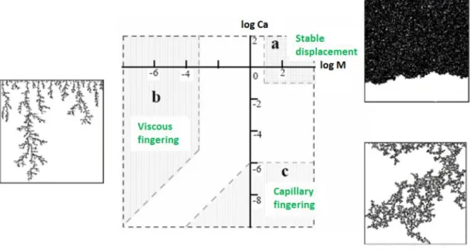
59 2.2.2.1 Capillary fingering regime for the invasion of water in a GDL
2.2.2.2 Transport of water in vapor form and condensation of water in a GDL 61
2.2.3 Models and simulations 62
2.2.3.1 Homogenized models 62
2.2.3.2 Pore-scale models 64
2.2.3.2.1 Pore network models 64
66
2.3 67
67 2.2.3.2.2 Full morphology model
Imaging techniques to study fuel cell materials 2.3.1 Imaging techniques
2.3.2 Quantitative use of images 69
2.3.2.1 Image processing and analysis tools 70
70 71 71 71 2.3.2.1.1 Filtering 2.3.2.1.2 Segmentation 2.3.2.1.3 Shape analysis 2.3.2.1.4 Mathematical morphology 2.3.2.1.5 Other algorithms 72 72 73 2.3.2.2 Image-based models and simulations 2.3.3
Virtual models of microstructures
2.3.4 Limitations of accessible information using imagery 73
73 73 75 75 2.3.4.1 Noise
2.3.4.2 Limited resolution and multi-scale structure of materials 2.3.4.3 Lack of contrast between some materials
2.3.4.4 Limited field of view and spatial variability of microstructures
2.3.4.5 Discretization effect 76
2.4 Bibliography 77
83
3.1 84
Numerical verifications of diffusive transport simulations Methodology
3.1.1.1.2 Diffusive transports simulations on pore networks 86 3.1.1.1.3 Calibration of the conductances on the pores and link geometries 88 3.1.1.1.3.1 Presentation of the problem of conductance calibration 88
3.1.1.1.3.2 Geometry-dependent conductance model 89
3.1.1.1.3.3 Calibration of the conductance model on the pores and links geometries 91
3.1.1.2 Direct simulations using the explicit jump method, EJ-Heat 92
3.1.1.2.1 Stationary heat equation 92
3.1.1.2.2 Discretization and solving 94
3.1.1.3 Regular pore networks 94
3.1.1.3.1 Properties of the unit cells 95
96 3.1.1.3.2 Properties of regular pore networks with random pore sizes
3.1.2 Test cases for simulations 98
98 99 3.1.2.1 Test case: layered medium
3.1.2.2 Test case: regularly spaced cylinders in a continuous
medium 3.1.2.3 Test case: GDL tomographic image 100
3.2 Results 101
3.2.1 Numerical verification of direct EJ-Heat simulations and simulations on pore networks extracted from
images 101
101 102 3.2.1.1 Test case: layered medium
3.2.1.2 Test case: regularly spaced cylinders in a continuous
medium 3.2.1.3 Test case: GDL tomographic image 105
106 107 3.2.1.3.1 Diffusive transport in the fluid phase and in the solid
phase 3.2.1.3.2 Diffusive transport in the fluid phase
3.2.1.3.3 Diffusive transport in the solid phase 108
109 3.2.1.4 Conclusion
3.2.2 Study of the diffusive transport properties of regular cubic pore networks 110 3.2.2.1 Regular cubic pore network model calibrated on the pores size distribution of a GDL 110
3.2.2.1.1 Calibration of the network 110
3.2.2.1.2 Effective diffusive transport properties of the regular network 111 3.2.2.2 Correlations between effective transport properties of solid and fluid phases 115 117 3.3 117 3.4 119 3.5 3.2.2.3 Conclusion Perspectives Conclusion Bibliographie 120
125 4.1.2 X-ray tomography
4.1.3 Image segmentation 126
4.1.3.1 Segmentation of air and solid 127
129 131 4.1.3.2 Distinction of binder and fibers
4.1.4 Ej-Heat direct simulation of diffusive transports
4.1.5 Bulk transport properties of materials constituting the GDL 131 132 4.1.5.1 Binary diffusion coefficients of several
gases 4.1.5.2 Electrical conductivity of bulk materials
133
4.2 Results 134
4.2.1 Experimental validation of simulations 134
4.2.1.1 Effective diffusivities 134
4.2.1.1.1 GDL TGP-H-060 134
4.2.1.1.2 GDL 24BA 136
4.2.1.2 Effective electrical conductivities 138
4.2.1.2.1 GDL TGP-H-060 138
140 4.2.1.2.2 24BA GDL
4.2.2 Additional simulation results 142
4.2.2.1 Spatial variability of GDL transport properties 142
145
4.3 145
4.4 146
4.5
4.2.2.2 Diffusivity of a GDL completely invaded by liquid water Discussion
Conclusion
Bibliography 147
Injection of liquid water into a GDL 149
5.1 Validation of pore network simulations of ex-situ water distributions in a gas diffusion layer of proton exchange
membrane fuel cells with X-ray tomographic images 150
5.2 164
5.3
Capillary pressure curve simulations
Conclusion 167 5.4 Bibliography 168 169 6.1 169 Water condensation in a GDL Methodology
6.1.1 Network pore model of condensation in a GDL 169
170 171 172 6.1.1.1 Algorithm for condensation of water coupled with mass and heat diffusive
transports 6.1.1.2 Vapor pressure at the liquid-gas interface 6.1.1.3 Diffusion of water vapor
6.2.1 Condensation simulations on Voronoi pore networks 177 6.2.1.1 Condensation simulations on a 3D Voronoi pore network 177 181
6.3 186
6.4 186
6.5
6.2.1.2 Condensation simulations on 2D Voronoi pore networks Perspectives
Conclusion
Bibliography 187
Study of virtual microstructures 189
7.1 Methodology 191
7.1.1 Optimal porous microstructures for the through-plane diffusive transport of gases and electrons 191
7.1.2 MPL-GDL assemblies 192
7.1.2.1 Generating virtual MPL-GDL assemblies 193
196 7.1.2.2 Apparent properties of GDL: analytical model on a simplified
geometry 7.1.3 Model of electrical contact resistances between GDL fibers 197 198 199 7.1.3.1 Generation of virtual GDL whose fibers are distinguished
individually 7.1.3.2 Algorithm to identify boundaries between distinct phases
7.1.3.3 Model of electrical contact resistances on 3D images
201
7.2 Results 201
7.2.1 Optimal cubic porous microstructures for through-plane diffusive transports of gases and electrons201
7.2.2 Properties of virtual MPL - GDL assemblies 204
204 205 7.2.2.1 Geometric analysis of the virtual microstructures
7.2.2.2 Simulation of the effective diffusive transport properties of the virtual microstructure
7.2.2.3 Apparent transport properties of the GDL 206
207 7.3 208 208 209 7.4 210 7.5
7.2.3 Model of electrical contact resistances between GDL fibers Perspectives
7.3.1 Optimization of microstructures 7.3.2 Generation of virtual microstructures Conclusion Bibliography 210 215 8.1 216 216 217 217 218 Conclusion Main results
8.1.1 Numerical verifications of diffusive transport simulations 8.1.2 Experimental validation of diffusive transport simulations 8.1.3 Injection of liquid water into a GDL
8.1.4 Water condensation in a GDL
9.1 222 9.2 223 223 225 226 9.3 228 228 228 230 9.4 232 232 233 235 Simulations tools on tomographic images
Probabilistic model for the variability of materials
9.2.1 Probabilistic model for MEA materials transport properties
9.2.2 Effect on performances of the spatial variability of the materials transport properties 9.2.3 Conclusion
Analytical calculations of the properties of the cubic unit cells of regular pore networks 9.3.1 Description of the geometry studied
9.3.2 Transport properties of the gas phase 9.3.3 Transport properties of the solid phase Constrictivity equation
9.4.1 Presentation of the constrictivity equation
9.4.2 Numerical verification of the constrictivity equation 9.4.3 Conclusion
GDL Gas Diffusion Layer
EDP Equation aux Dérivées Partielles IBM Immersed Boundary Method JPS Journal of Power Sources LBM Lattice Boltzmann Method MIP Mercury Intrusion Porosimetry MPL Microporous Layer
MRI Magnetic Resonance Imaging OCV Open Circuit Voltage
PEM Polymer Electrolyte Membrane
PEMFC Polymer Electrolyte Membrane Fuel Cell PTFE Polytetrafluoroethylene
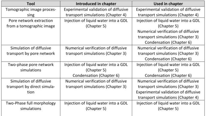
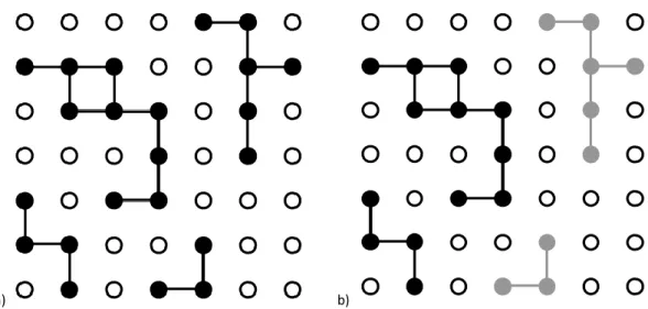
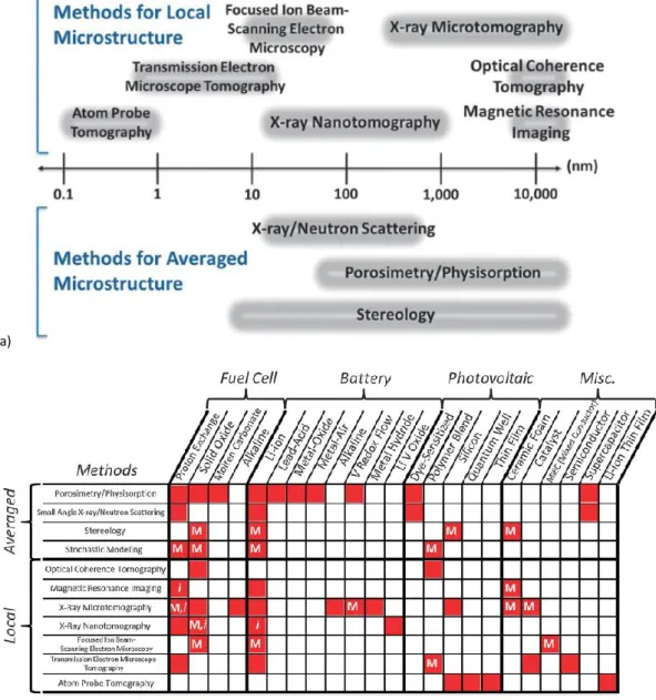
Figure 1.1 Schematic diagram of a proton-exchange membrane fuel cell. ... 31 Figure 1.2 Typical polarization curve of a PEM fuel cell. ... 33 Figure 1.3 Diagram illustrating the operation of a PEMFC fuel cell cell and sectional view of its constituents. Figure extracted from [Robin2015]... 35 Figure 1.4 Sectional view of an electrode membrane assembly. Image made with a scanning electron microscope (SEM). Image from [CHAMEAU2010]. ... 35 Figure 1.5 SEM image of porous materials used in PEM fuel cell electrodes. a) catalytic layer b) gas diffusion layer. Images from [CHAMEAU2010]. ... 36 Figure 1.6 GDL in contact with a bipolar plate. Image from [Straubhaar2015]. ... 37 Figure 1.7 Transport of reactive gases, electrons and water vapor in a GDL inserted between a bipolar plate and a catalytic layer (the microporous layer is not shown). ... 37 Figure 1.8 Sectional view of a GDL Freudenberg H2315T10A with MPL, obtained by scanning electron microscopy on a sample coated with epoxy resin and then polished [CHAMEAU2010]. ... 38 Figure 1.9 Diagram of transports in a GDL, for an in-situ fuel cell configuration. The GDL is inserted between a bipolar plate (in black) and a catalytic layer. a) diffusive transport of electrons or gases b) transport of water injected in liquid form into the GDL c) condensation of water coupled to a diffusive transport of water vapor. ... 41 Figure 1.10 Tools used to process tomographic images and perform simulations on tomographic images. ... 42 Figure 2.1 Classification of the invasion patterns during fluid drainage experiments in a porous media, as a function of the capillary number and the ratio of the viscosities of the wetting and non-wetting fluids. Taken from [Ewing2001]. ... 60 Figure 2.2 Comparison of saturation profiles obtained using a generalized Darcy model at the homogenized scale and a pore network model at the pores scale. Figure extracted from [Rebai2009]. ... 63 Figure 2.3 Explanatory diagram of the percolation invasion algorithm. At each stage, water invades the link which has the lowest capillary pressure threshold. When the network is uniformly hydrophobic, this leads to invading the broadest links first. Figure extracted from [Straubhaar2015]. ... 65 Figure 2.4 Comparison of percolation invasion and pure percolation on a square lattice. (A) Pure percolation. Black areas are active regions. B) invasion percolation. The black areas are invaded regions because they are active for pure percolation and because they are connected by a continuous path to the injection face, on the left. The gray areas are not invaded because they are not connected to the injection face. Figures from [Gostick2008-thesis]. ... 66 Figure 2.5 a) Classification of techniques used to image materials for energy, depending on the resolution and the spatially resolved or averaged nature b) state of the art in the use of these imaging techniques for different materials for energy. Figures from [Cocco2013]... 68 Figure 2.6 Diagram of an X-ray tomography device. Taken from [Straubhaar2015]. ... 69 Figure 2.7 SEM images of GDL. From left to right and from top to bottom: increasing zoom. The characteristics of the microstructure are not the same at all scales. Images taken by Marco Bolloli, CEA. ... 74 Figure 2.8 3D images of virtual GDL microstructures at the same zoom level, which vary randomly. 76 Figure 3.1 Illustration of the pore network extraction method on two types of GDL images. A-1) tomographic image of a GDL b-1) pores extracted from the porous phase of this image, one color per pore c-1) extracted pore network. The pore network is shown in the form of balls, although the pores are volumes of any shape.
at the boundary between two pores. D-2) Extracted network. Pore are represented as balls, with a color depending on the phase. Blue: air, white: fibers, red: binder. The links are represented by lines. .... 85 Figure 3.2 Several discretizations for the same microstructure. A) microstructure composed of 4 distinct phases, indicated by different colors. B) discretization of the microstructure on a grid of voxels c) diagram of a pore network extracted from the microstructure. Each pore corresponds to a region of the image. Two pores are connected by a link if the regions of the pores in the image have a common boundary. ... 87 Figure 3.3 Pores and cubic links conventionally used in pore networks. ... 88 Figure 3.4 3D visualizations of pore extracted by watershed segmentation from an image of a GDL 24BA. Blue and red pores are pairs of pores linked by a link. Links are not shown on these images. ... 89 Figure 3.5 Illustration of the discretization of a microstructure on a regular grid of voxels. A) microstructure composed of 4 phases (one color per phase). B) superposition of the voxel grid and the microstructure. Each voxel is assigned the conductivity of the dominant phase in the volume of this voxel. C) voxel grid obtained. The relation with a network representation is illustrated by connecting the neighboring voxels by edges. At the interfaces between the phases (in dotted lines), the value of the conductivity generally undergoes a jump. ... 93 Figure 3.6 Diagrams of a regular cubic pore network, composed of cubic pores and parallelepiped links distributed on a regular 3D grid. A) 2D section of a 3D cubic pore network. B) 3D representation of a unit cell. C) slice view of a unit cell. ... 95 Figure 3.7 3D rendering of the microstructure used for the test case layered medium... 98 Figure 3.8 Microstructures used for the test case: cylinders regularly spaced in a continuous medium. ... 99 Figure 3.9 Tomographic image of a compressed GDL 24BA. ... 100 Figure 3.10 A) microstructure used for the test case array of cylinder b) pores extracted from the image c) pore network extracted. Pore are represented as balls, although the pores shapes considered in the conductances are not balls. ... 101 Figure 3.11 Comparison of numerical methods on the case test layered medium, for the effective conductivity in the direction parallel to the layers. The bulk conductivity of one phase is set to 1, the bulk conductivity of the other phase is either 1, 0.1 or 0.01. ... 102 Figure 3.12 A) microstructure used for the test case array of cylinder b) pores extracted from the image c) deviation around the mean temperature field calculated by EJ-Heat. ... 102 Figure 3.13 Comparison of numerical methods on the case test cylinder array, for the effective conductivity in the direction perpendicular to the cylinders. The bulk conductivity of the homogeneous medium is set to 1, the bulk conductivity of the cylinders is either 1, 0.1 or 0.01. ... 103 Figure 3.14 A) Effective conductivity values calculated by EJ-Heat. B) and c) relative deviations between the effective conductivities calculated with Ej-Heat and with the Rayleigh formula. ... 104 Figure 3.15 Pore network extracted from fluid and solid phases of a compressed 24BA image. A) "stick and balls" representation of the pore network. The red balls represent the pores of the fluid phase, the blue balls the pores of the solid phase, the yellow segments the links. B) and c) Sectional view of the extracted pores. D) zoom on a part of the view in section b. ... 105 Figure 3.16 Simulation results on a tomographic image of 24BA. The conductivity of the two phases is assumed to be the same. ... 106 Figure 3.17 Simulation of effective diffusivity on a tomographic image of a GDL 24BA. The bulk diffusivity of the fluid phase is assumed to be non-zero, that of the solid phase is assumed to be zero. ... 107
Figure 3.19 Distributions of pore sizes (a) and constriction sizes (b) based on a compressed 24BA tomographic image. The pores and constrictions are extracted from the image by watershed segmentation with h-Maxima markers, h = 4 voxels. ... 111 Figure 3.20 Sensitivity study of the effective transport properties of regular networks. On the left, dimensionless pore size distribution. Three Weibull distributions are studied, with different shape parameters and thresholds. On the right, the Wiener bounds on the effective diffusivity in the gas phase and the effective conductivity in the solid phase as a function of k. EJ-Heat simulations of the effective properties of a compressed GDL 24BA are shown as points for comparison. ... 112 Figure 3.21 Comparison of numerical methods for the effective diffusivity of compressed GDL 24BA. A) effective diffusivity in the plane. B) Effective diffusivity through the thickness. ... 113 The upper Wiener bound for relative diffusivity is the same in all three cases, 0.31. This corresponds to a network in which the pores are aligned in the direction of transport. Note that this value is close to the value predicted by the Bruggeman formula, 𝐷𝑒𝑓𝑓𝐵𝑟𝑢𝑔𝑔𝑒𝑚𝑎𝑛𝜀 = 0.5 = 0.35. The lower Wiener bound varies between 0.05 and 0.13, depending on the pore size distribution chosen. We considered the value 0.05 for Figure 3.24, which provides the broadest diffusivity range. ... 113 Figure 3.23 A) relative effective diffusivity as a function of porosity, calculated for the whole range of u and k. B) relative effective conductivity as a function of porosity. Relative means adimensioned by the bulk transport property of the phase. ... 115 Figure 3.24 Correlation between the effective conductivity of the solid phase and the effective diffusivity of the gas phase. In blue: cubic mesh. In red: Ej-Heat simulations on a 24BA GDL 3D image. ... 116 Figure 4.1 Tomographic images of GDL obtained on a CEA industrial tomography system. A) image of uncompressed GDL 24BA (slices). B) GDL image TGP-H-060 uncompressed (slices). ... 126 Figure 4.2 X-ray tomographic image of uncompressed TGP-H-060 taken at CEA. A) raw image, with adjusted contrast b) 3D anisotropic diffusion filter applied to the image a. C) solid phase obtained after thresholding of the image b. ... 127 Figure 4.3 Images of GDL after segmentation of air and solid. A) Uncompressed 24BA image b) Compressed 24BA image C) Uncompressed TGP-H-060 image d) Compressed 24BA image. The images a and c were carried out by the CEA on an industrial tomography system. The b and d images were taken by the Paul Scherrer Institute on a synchrotron. ... 128 Figure 4.4 A), b): Compressed 24BA images with binder identified by morphological segmentation. Fibers in red, binder in pink salmon. (A) complete sample. B) zoom on the surface of the GDL. C) Images of TGP-H-060 with segmented binder. D) uncompressed 24BA with segmented binder. ... 130 Figure 4.5 Images of the deviation around the mean concentration field, simulated on the microstructure to calculate the through-plane diffusivity. The microstructure is obtained by X-ray tomography on a compressed 24BA subsample. The colors represent the deviation from the average concentration field. Color code: dark red = high value, dark blue = low value. ... 134 Figure 4.6 Effective relative diffusivity of a Toray H-060. A) Comparison between experiment and simulation for in-plane and through-plane effective diffusivities Figure created by the author from data in [Rashapov2016], [Kramer2008] b) Sensitivity of the simulations to the bulk diffusivity of the binder.135 Figure 4.7 Relative effective diffusivity of a GDL 24BA. A) Comparison between experiment and simulation for in-plane and through-plane effective diffusivities Figure created by the author from data in [Rashapov2016] b) Sensitivity of the simulations to the bulk diffusivity of the binder. ... 137 Figure 4.8 Images of the deviation around the mean electric potential field simulated on the microstructure to calculate the through-plane electrical conductivity. The microstructure is obtained by X-ray tomography on a compressed 24BA subsample. The colors represent the deviation from the mean electrical potential. Color code: dark red for high values, dark blue for low values. ... 138
Figure 4.10 Effective electrical conductivity of GDL 24BA. A) Comparison between simulations and experimental measurements. The experimental points were carried out at the CEA at 1 MPa and 5 MPa. The simulations were carried out with a binder conductivity either equal to zero or equal to the conductivity of the fibers (61000 S / m). B) Sensitivity of the simulations of effective electrical conductivity with respect to the bulk conductivity of the binder. ... 141 Figure 4.11 Porosity of sub-samples of 24BA whose size varies. The width of the sample on the abscissa is given in number of voxels. The size of a voxel on this image is 2.2μm. ... 142 Figure 4.12 a) Image of GDL 24BA. B) 9 sub-samples of this image, decomposed per a 3 * 3 grid. .. 143 Figure 4.13 Effective through-plane properties of compressed GDL 24BA subsamples. A) effective diffusivity as a function of the effective conductivity. B) effective conductivity as a function of the solid fraction in the sample. C) effective diffusivity as a function of the gas fraction of the sample. ... 144 Figure 5.1 Full morphology simulation on a sub-sample of the 24BA image at different pressure levels (increasing pressure from left to right). The water is blue, the GDL is red. We see that the saturation of water increases when the pressure increases. ... 164 Figure 5.2 Comparison between experiment and full morphology simulation for capillary pressure curves. Two types of GDL are studied: GDL Toray TGP-H-060 (in green) and GDL SGL 24BA (in red). Figure created by author from data in [Lamibrac2016]. ... 165 Figure 5.3 A) Variability of capillary pressure curves on sub-samples of GDL 24BA. In red, simulation on the complete sample. In blue, simulations on sub-samples. B) Simulations of capillary pressure curves, injecting water into the 24BA by a face or the opposite face. In red, capillary pressure curves for the complete sample. In blue, curves obtained on a sub-sample. ... 165 Figure 5.4 Comparison between the Leverett model and full morphology simulations for the capillary pressure curve. ... 167 Figure 6.1 Boundary conditions for the transport of water vapor by diffusion. Figure extracted from [Straubhaar2015]. ... 173 Figure 6.2 Boundary conditions for the transport of heat. Figure extracted from [Straubhaar2015].174 Figure 6.3 Voronoi mesh generated from a set of random points. The cells of the mesh are represented in color, the points from which the mesh is generated are represented in black. ... 175 Figure 6.4 A porous microstructure generated from a Voronoi mesh. This microstructure is composed of two regions having different pore sizes. The pores are the polyhedral meshes of the Voronoi mesh. The edges of the meshes, thickened, constitute the solid. Figure created by author and also used in [Prat2015].176 Figure 6.5 Condensation results on an isotropic Voronoi 3D network. Thickness of the GDL: 300μm. Width: 2mm, including 1mm under the rib, thickness: 1mm. Average diameter of a pore: 30μm. The in-plane profiles are profiles along the channel-rib-channel direction. ... 179 Figure 6.6 Condensation results on an isotropic 2D Voronoi pore network representing a GDL without a MPL. ... 183 Figure 6.7 Condensation results on an anisotropic 2D Voronoi pore network representing a GDL without a MPL. ... 185 Figure 7.1 Diagrams of cubic porous structures used for microstructure optimization. A) 3D representation. B) 2D slice. ... 192 Figure 7.2 SEM image of a MPL-GDL assembly, SGL 24BC. The lighting is not uniform, which explains why the center of the image is darker than the sides. ... 193
Figure 7.4 Virtual MPL-GDL assembly a) 3D rendering b) sectional view of the interpenetration zone c) 3D rendering of a larger virtual MPL-GDL assembly, not studied here. ... 194 Figure 7.5 Section views of virtual MPL-GDL assemblies. Radius of the balls used to simulate MPL penetration, from a to g: 14, 16, 18, 20, 25, 30, 70 (in voxels). The thickness of MPL is varied to maintain a volume fraction of MPL of 50% in the image regardless of the level of penetration. ... 195 Figure 7.6 Schematic of the simplified MPL-GDL assembly microstructure used for analytical calculations. ... 196 Figure 7.7 a) GDL with the fibers identified separately. B) Same GDL after adding the binder (in red).198 Figure 7.8 a) Contacts between the different elements of the image (3D view and section view). B) Contacts divided into 2 categories: yellow for contacts between fibers and binder, white for contacts between fibers. The contacts between the fibers are often cylindrical. It is an artifact related to the process of building virtual GDL, which inserts a new fiber by replacing the voxels already occupied. C) Final image where the locations of the different fibers, the binder and the contacts are known. The contacts between fibers and between binder and fibers are shown in white on this image. The colors correspond to the fibers and the binder. . 200 Figure 7.9 Properties of porous cubic cells for the optimization problem. A) Correlation between electrical conductivity and diffusivity. The optimal Pareto structures are in red. B) Geometric parameters of Pareto optimal cells. C) parallel coordinates graph of geometric parameters and effective properties. The yellow lines correspond to the optimal microstructures in the Pareto sense, the blue lines to non-optimal structures. ... 202 Figure 7.10 Comparison between the effective diffusive transport properties of the cubic cells and several commercial GDLs. ... 203 Figure 7.11 a) Volume fraction of MPL in GDL, as a function of the inverse of the radius of the balls used to simulate MPL penetration. b) MPL penetration distance in GDL, as a function of the inverse of the radius of the balls. ... 204 Figure 7.12 Effective diffusive transport properties of virtual MPL-GDL assemblies, obtained by direct Ej-Heat simulations. ... 205 Figure 7.13 Effective apparent properties of the GDL, as a function of the volume fraction of MPL in GDL. ... 206 Figure 7.14 Effect of contact resistances between fibers on the anisotropy of electrical conductivities of virtual GDLs. ... 207 Figure 9.1 AME in blue, bipolar plates in gray. Slice view. We have decomposed the AME into elementary patterns (separations in red) for the purposes of modeling the spatial variability between patterns. 𝐶𝑑𝑖𝑓𝑓(𝑘) denotes the through-plane effective diffusivity. We assume that there are no exchanges through the orange separations. The elementary patterns are thus generators in parallel in the fuel cell electrical circuit (in black, an example of an electrical circuit with a resistance). ... 224 Figure 9.2 a) 2D section of the cubic lattice. B) 3D representation of a unit cell. ... 228 Figure 9.3 Diagram of the cubic unit cell. The three sections used to calculate the properties of this unit cell are shown. Sections 1 and 2 are shown once for simplicity, but they are in fact symmetrical with respect to Section 3. ... 229 Figure 9.4 Comparison between constrictivity equation and analytical formulas for the effective properties of diffusive transport on a regular cubic lattice. Left: transport in the gas phase. Right: transport in the solid phase. From top to bottom: k = 0.1, k = 0.5, k = 0.9, ratio of constrictivity equation and analytical calculations. ... 234
List of tables
Tableau 1-1 List of the numerical tools used, chapters in which they are introduced and chapters in which they are used... 42 Tableau 1-2 Implemented approach for the validation and exploitation of simulation tools that use images of porous microstructures. ... 43 Tableau 2-1 Imaging methods used to visualize water in PEM fuel cells. Table adapted from [Kim2013] ... 57 Tableau 3-1 Profile shapes of the links, used for conductance calculation. ... 91 Tableau 3-2 Effective properties of several GDL calculated on tomographic images by direct simulation Ej-Heat in Chapter 4. The effective diffusivities are normalized by the bulk diffusivity of the gas, the effective conductivities by the bulk conductivity of the solid (fibers and binder are indiscriminated). ... 114 Tableau 4-1 Porosity of GDL calculated on images and experimentally measured. The experimental measurements given here are data provided by the manufacturers of GDL. ... 129 Tableau 6-1 Parameters used in the simulations of water condensation in the 3D Voronoi pore network. ... 177 Tableau 6-2 Parameters used in simulations of water condensation in pore networks constructed from a 2D Voronoi mesh. ... 181 Tableau 7-1 Bulk properties used for EJ-Heat simulations on virtual MPL-GDL assemblies. ... 195 Tableau 7-2 List of studied cases and their parameters, for electrical contact resistance simulations. ... 201
List of equations
Équation 1.1... 31 Équation 1.2... 32 Équation 1.3... 32 Équation 1.4... 33 Équation 1.5... 33 Équation 1.6... 34 Équation 1.7... 34 Équation 2.1... 48 Équation 2.2... 49 Équation 2.3... 49 Équation 2.4... 49 Équation 2.5... 52 Équation 2.6... 52 Équation 2.7... 53 Équation 2.8... 55 Équation 2.9... 58 Équation 2.10... 60 Équation 2.11... 60 Équation 2.12... 60 Équation 2.13... 61 Équation 2.14... 62 Équation 2.15... 62 Équation 2.16... 62 Équation 2.17... 62 Équation 2.18... 63 Équation 2.19... 63 Équation 3.1... 86 Équation 3.2... 86 Équation 3.3... 87 Équation 3.4... 87 Équation 3.5... 88 Équation 3.7... 90 Équation 3.8... 90Équation 3.9... 92 Équation 3.10... 93 Équation 3.11... 93 Équation 3.12... 93 Équation 3.13... 94 Équation 3.14... 95 Équation 3.15... 96 Équation 3.16... 96 Équation 3.17... 96 Équation 3.18... 97 Équation 3.19... 97 Équation 3.20... 97 Équation 3.21... 99 Équation 3.22... 99 Équation 3.23... 100 Équation 3.24... 110 Équation 3.26... 119 Équation 5.1... 166 Équation 5.2... 166 Équation 5.3... 166 Équation 6.1... 171 Équation 6.2... 171 Équation 6.3... 172 Équation 6.4... 172 Équation 6.5... 172 Équation 6.6... 173 Équation 6.7... 174 Équation 6.8... 175 Équation 7.1... 191 Équation 7.4... 196 Équation 7.5... 196 Équation 7.6... 196 Équation 7.7... 197 Équation 7.8... 197
Équation 7.9... 206 Équation 7.10... 206 Équation 9.1... 224 Équation 9.2... 224 Équation 9.3... 225 Équation 9.4... 228 Équation 9.5... 228 Équation 9.6... 230 Équation 9.7... 232 Équation 9.8... 232
Introduction
Hydrogen used as an energy carrier is a promising solution for reducing greenhouse gas emissions. Indeed, the dihydrogen makes it possible to store large quantities of energy in a totally decarbonized way. The energy is stored in chemical form in dihydrogen molecules, 𝐻2. When the dihydrogen, 𝐻2, reacts with the oxygen
from the air, 𝑂2, to form water, 𝐻2𝑂, the chemical energy is released and can be used. The environmental
emis-sions from this chemical reaction are water and heat.
The dihydrogen does not exist in the natural state; therefore, it must be produced. There are many methods to produce dihydrogen [Dincer2015]. These vary in terms of costs and emissions of greenhouse gases. When dihy-drogen is produced from decarbonized energy, for example by electrolysis of water from electricity of renewable origin, or by reforming biogas, the carbon balance of the production of dihydrogen is quasi-neutral. This explains the interest of the dihydrogen from the environmental point of view.
Reducing greenhouse gas emissions is crucial to keeping global warming below 2°C. Beyond this threshold, risks to humanity are manifold: food insecurity due to deteriorating crop yields and declining animal populations, population migration due to rising sea levels, increased frequency of extreme climate events [IPCC2014]. Recall that global warming is due to greenhouse gas emissions during the industrial period, from 1870 to the present day, driven by the use of fossil fuels, which contributed to develop the economies of the industrialized countries
[Paris2015]. 𝐶𝑂2 emissions are still increasing worldwide [IEA2013]. These increases are mainly due to economic
growth in emerging countries [IPCC2014]. To reduce global greenhouse gas emissions while ensuring the eco-nomic development of emerging countries, ecoeco-nomic, social and technological changes are required to drasti-cally reduce emissions per gross domestic product (GDP). In Europe and France, the objective is to reduce green-house gas emissions of 1990 by a factor of 4 by 2050 [EuropeEnergy2011] [Tuot2007].
The storage of electric energy has an essential role to play in this context. A primary utility of storage is to ensure the stability of electrical networks in the presence of intermittent renewable energies [USStorage2013]. Having better means of energy storage would thus increase the share of renewables in electricity generation. Storing large quantities of energy is also important for the transport sector. This sector is responsible for more than 10% of greenhouse gas emissions [IEA2014]. Dihydrogen is relevant for transport because it has a high energy density, which allows to store large quantities of energies in a vehicle with a moderate mass [Durbin2013].
Fuel cells are the electrochemical devices used to control the chemical reaction between dihydrogen and dioxy-gen so that energy is released primarily in useful electrical form. Fuel cells therefore play an essential role in the use of dihydrogen as an energy carrier. Fuel cells account for a significant portion of the costs of using dihydro-gen. They are the subject of much research aimed at reducing their cost, increasing their durability and improving their performance.
This thesis is part of a global approach to modeling fuel cells to improve the competitiveness of this technology. The objective of modeling is to improve our understanding and control of the physical phenomena taking place in fuel cells. In particular, transport in porous electrodes plays a crucial role in the operation of fuel cells. In this thesis, we concentrate on a porous material involved in the electrodes of fuel cells, gas diffusion layers (GDL). GDLs have many functions, including allowing simultaneous transport of gases, electrons, heat and water in steam and liquid form. The microstructure of the GDL plays a crucial role on the compromises between the multiple functions of the GDL and the efficiency of transport in the electrodes. The objective of this thesis is to
model the transport properties of GDLs, to better know them and to be able to optimize them. Modeling is an essential tool because the transport properties of GDLs are often difficult to measure experimentally because of their small thickness (300 μm). To better understand the effect of the microstructure of porous materials on transport, we take advantage of the advances in imaging techniques that allow us to know precisely the micro-structure of porous electrode materials today. We concentrate on a component of the electrodes, the GDLs, because we have high-quality images of their microstructures obtained by X-ray tomography.
The remainder of this introduction consists of a presentation of the general operation of fuel cells and of the stakes represented by transport in the gas diffusion layers. We then present the objectives of this thesis and the approach implemented.
1.1 The proton exchange membrane fuel cell technology
In this section, we present the principle of proton exchange membrane (PEM) fuel cells, the different types of losses that occur in the cells, the materials that make up the core of the cells, and finally the problem of the water management in the cells.
1.1.1 General operation
The fuel cell is for the dihydrogen what the combustion engine is for oil: the device by which the chemical energy of hydrogen gas is converted into usable energy. We describe here the principle of operation of a PEM fuel cell. The chemical energy contained in the 𝐻2 dihydrogen molecules is released during the oxidation-reduction
reac-tion with 𝑂2 dioxygen. The equation of this reaction is :
2𝐻2+ 𝑂2→ 2𝐻20 Équation 1.1
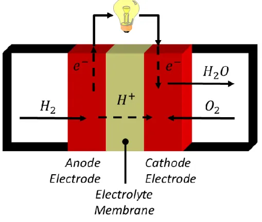
If this reaction took place in the open air, by direct combustion of the dihydrogen in the dioxygen, the energy would be violently released in the form of heat. For the reaction to produce electricity, it is controlled in an electrochemical device, the fuel cell. Figure 1.1 illustrates the principle of proton exchange membrane fuel cells.
The reaction is decomposed into two half-reactions occurring in two separate compartments, the anode and the cathode.
At the anode, the dihydrogen decomposes into protons and electrons, in contact with a catalyst. This reaction is endothermic at normal operating temperatures.
2𝐻2→ 4𝐻++ 4𝑒− Équation 1.2
At the cathode, protons and electrons combine with the dioxygen to form water, with the aid of a catalyst. This reaction is exothermic at normal operating temperatures.
02+ 4𝐻++ 4𝑒−→ 2𝐻20 Équation 1.3
The two reactive gases 02 and 𝐻2 are in principle never in direct contact. They are kept separated by a solid
electrolyte, the proton exchange membrane (PEM), almost impermeable to gases but letting the protons pass. The electrons are guided by electrical conductors to an external electrical circuit, so that their energy is used in electrical form. The fuel cell is fed continuously with 𝐻2 and 02, which allows the production of electricity
con-tinuously.
Although the reactive gases are not in physical contact, the reaction nevertheless occurs because these gases are indirectly in electrical contact, via the electrons and the ions which can circulate between the anode and the cathode. The molecules see electrical potentials linked to the oxidation-reduction couple, allowing the release or capture of electrons.
1.1.2 Performance and losses
The chemical energy of gases is converted largely into electrical energy in the fuel cell. But, because of a certain number of physical phenomena which we describe in this section, this conversion is not perfect. Losses occur and reduce system performance.
Generation of electricity by the fuel cell is measured by the cell voltage, 𝑉𝑐𝑒𝑙𝑙, and by the quantity of current
produced, I. When the current is zero, the theoretical voltage of the cell corresponds to the Nernst electrochem-ical potential of the two half-reactions, 𝑉𝑁𝑒𝑟𝑛𝑠𝑡= 1.229 𝑉 at 25°C and normal pressure conditions. The voltage
at zero current is denoted 𝑉𝑂𝐶𝑉 in the following. The voltage 𝑉𝑂𝐶𝑉 measured is slightly lower than the theoretical
value 𝑉𝑁𝑒𝑟𝑛𝑠𝑡, because of the small amounts of 02 and 𝐻2 which pass through the membrane [Vilekar2010].
Figure 1.2 Typical polarization curve of a PEM fuel cell.
When current is generated, additional voltage losses occur. The voltage losses can be decomposed into activation polarization 𝜂𝑎𝑐𝑡(𝑖), ohmic polarization 𝜂𝐼𝑅 and concentration polarization 𝜂𝑐𝑜𝑛𝑐 [O'Hayre2009].
𝑉𝑐𝑒𝑙𝑙(𝑖) = 𝑉𝑂𝐶𝑉− 𝜂𝑎𝑐𝑡(𝑖) − 𝜂𝐼𝑅(𝑖) − 𝜂𝑐𝑜𝑛𝑐(𝑖) Équation 1.4
The activation losses are related to the kinetic limits of the chemical reaction. For the reaction to occur, reactive species and intermediate species must overcome several energetic barriers. The electrical potential of the cell affects the ability of these species to overcome barriers, which leads to a relationship between cell potential and reaction rate. The relationship between current and resulting voltage can be described by the Tafel equation:
𝜂𝑎𝑐𝑡 = 𝑅𝑇 𝑎𝑛𝐹𝑙𝑛 ( 𝑖 𝑖0 ) Équation 1.5
Where F is the Faraday constant, R is the universal constant of the perfect gases, T is the reaction temperature, α is the electron transfer coefficient, n is the number of electrons transferred per reaction and 𝑖0 is the exchange
current density. The exchange current density depends on the activity of the catalysts and the concentration of reactants in the catalytic layers.
The ohmic losses 𝜂𝐼𝑅 are due to the ohmic resistance occurring during transfer of protons and electrons in
ma-terials. They are expressed by the following equation:
𝜂𝐼𝑅= 𝑖×(𝑅1+ 𝑅2+ ⋯ ) Équation 1.6
where 𝑅1, 𝑅2, … are the ohmic resistances of the different materials. The largest ohmic losses are caused by the
transport of protons in the membrane and the electrical contact resistances between the battery components. The concentration losses are related to the fact that when the current density is high, the gas transfers through the electrode have difficulty in supplying the reactive gases sufficiently quickly. This leads to a reduction in the concentration of the reactants at the level of the catalysts, which results in a decrease in the local exchange current density and thus in additional activation losses. The current of the cell to which the reactive gas concen-tration reaches zero is called the limit current density, 𝑖𝐿. It depends on the effective diffusion coefficient of the
dioxygen in the porous materials of the cathode and the concentration of dioxygen in the channel bringing the dioxygen to the surface of the cathode. The concentration overvoltage can be expressed by the following formula
[Barbir2005]: 𝜂𝑐𝑜𝑛𝑐= 𝑅𝑇 𝛼𝑛𝐹𝑙𝑛 ( 𝑖𝐿 𝑖𝐿− 𝑖 ) Équation 1.7
The transport of reactive gases through the electrodes is limited by several factors. The diffusion of oxygen is slower than that of dihydrogen, because on the one hand its concentration is generally lower because it is con-tained in the air and because on the other hand it is a heavier molecule therefore its binary diffusion coefficient is lower. The effective diffusion coefficient in the porous medium also depends on the microstructure of the electrodes. Finally, when much water is produced by the cell, the water tends to condense in the GDL and fill the pores, which limits the access of gases.
In this thesis, we concentrate on the concentration losses due to the transfer of species and the ohmic losses due to the transfer of electrons in a porous material of fuel cell, the gas diffusion layer.
1.1.3 Materials
The core of the cell is composed of two electrodes, anode and cathode, separated by a membrane. The elec-trodes are formed from several layers: catalytic layer and gas diffusion layers (GDL). Figure 1.3 illustrates sche-matically the exchanges between these different layers and the exchanges between the core of the stack and the bipolar plates situated on either side. The role of bipolar plates is to supply reactive gases to the core of the cell, to capture the electrons produced at the anode and to return them to the cathode, and to evacuate the heat and water produced in the core of the cell. Figure 1.4 shows a cross-sectional view of a real membrane-electrode assembly (MEA). We describe here in detail the materials constituting the MEAs.
Figure 1.3 Diagram illustrating the operation of a PEMFC fuel cell cell and sectional view of its constituents. Figure extracted from [Robin2015].
Figure 1.4 Sectional view of an electrode membrane assembly. Image made with a scanning electron microscope (SEM). Image from [CHAMEAU2010].
The role of the membrane is to be impermeable to the gases 𝐻2 and 02, as far as possible, but to transport the
𝐻+ ions. This selective permeability is obtained by the material of the membrane, which has different physical and chemical interactions with gas and protons. The membrane consists of a proton-conducting ionomer. This ionomer is often Nafion, a fluoropolymer, consisting of fluorine carbon chains, providing mechanical strength and resistance to acidity, and of hydrophilic 𝑆𝑂3𝐻 groups [Peighambardoust2010]. The Nafion has the possibility
of nanostructuring to form nanometric conduits filled with water, through which the protons can circulate thanks to their affinity with the water molecule, by hoping or diffusion [Peighambardoust2010]. The level of hydration of the membrane has a significant impact on its effective proton conductivity. Therefore, it is necessary to main-tain a cermain-tain humidity near the membrane [Ji2009]. Water can circulate through the membrane between the anode and the cathode, through electro-osmosis and diffusion [Kraytsberg2014].
Anodic and cathodic catalytic layers are the site of electrochemical reactions. These layers are located on either side of the membrane. The catalytic layers are composed of platinoid catalysts supported by carbon. Chemical reactions occur when the gases reach the surface of the catalysts. To maximize the chemical reaction rate, the catalytic layers have a microstructure that maximizes the developed surface area per unit volume. To reach high surfaces, the catalysts are formed of grains of a few nanometers in diameter. The carbon supports are made of grains of carbon black, which allows to reach specific surfaces of 10 to 1000 m² per gram. The role of the carbo-naceous support is to mechanically support the catalyst and to conduct the electrons required for the oxidation-reduction reactions. Proton-conducting ionomer (often Nafion) is added to the catalytic layers to conduct the protons to or from the membrane. The catalytic layers are produced by coating an ink on the membrane or on the diffusion layers. Their thickness generally varies between 5 μm and 30 μm. Figure 1.5 a) shows SEM images of the microstructure of the catalytic layer. The exact microstructure of the catalytic layers is the product of complex interactions between carbons, Nafion, catalysts and chemical additives used in ink. It is a porous micro-structure, the pores of which typically measure between 5 nm and 200 nm.
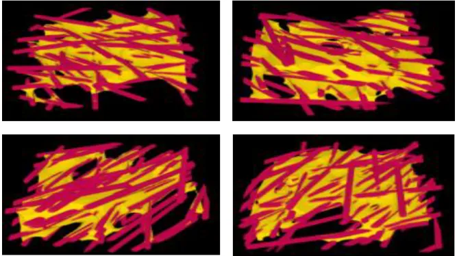
Figure 1.5 SEM image of porous materials used in PEM fuel cell electrodes. a) catalytic layer b) gas diffusion layer. Images
from [CHAMEAU2010].
The diffusion layers are located between the bipolar plates and the catalytic layers. Figure 1.6 shows how a bi-polar plate and a GDL are in contact. The role of the GDLs is to homogenize the transfers between the bibi-polar plate and the catalytic layer. Indeed, the GDLs allow the gases to reach the catalytic zones located under the ribs of the bipolar plate, leaving a thickness between ribs and catalytic layer. GDLs also have a mechanical role. They protect, by deforming, the catalytic layers and the membrane when the bipolar plates are compressed against the MEA to obtain good electrical contact.
Figure 1.6 GDL in contact with a bipolar plate. Image from [Straubhaar2015].
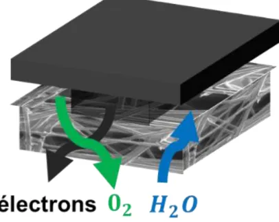
The GDLs are crossed by flows of reactive gas, heat and electrons. To this are added the flows produced at the cathode. To allow these flows, GDLs are porous materials. The electrons circulate through the electrically con-ductive solid phase. Reactive gases and water circulate through the pores. The thickness of the GDL is very thin (~150-300 μm) so that the transport resistances through the thickness of the GDL (through-plane) are minimized. Transport in the plane of the GDL (in-plane) allow the gases to reach the areas beneath the teeth of the bipolar plates. Transfers in GDL to and from the bipolar plate take place in two distinct zones: electrons circulate through the rib of the bipolar plate, in contact with the GDLs, while the gases flow through the channels of the bipolar plate, in contact with the GDLs too. Figure 1.7 shows these transfers in GDL in the presence of a bipolar plate.
Figure 1.7 Transport of reactive gases, electrons and water vapor in a GDL inserted between a bipolar plate and a catalytic layer (the microporous layer is not shown).
Figure 1.5 b) shows a SEM image of the microstructure of a GDL. The GDLs are composed of carbon fibers whose diameter is between 6 and 10 μm. The fibers are held together by a carbon binder (carbonaceous binder). A hydrophobic treatment involving PTFE (Teflon) is often added to limit the accumulation of water in GDL. The distribution of this treatment is often non-uniform, as it is distributed mainly in the surface layers of the GDL.
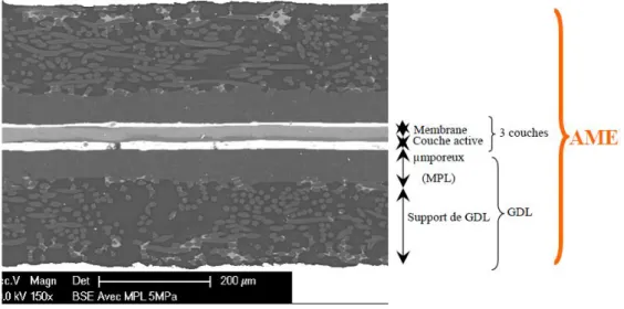
The porosity of GDL is between 70 and 90% [Rashapov2015]. The pore diameters are of the order of a few tens of micrometers. The physical properties of GDL are anisotropic because of the microstructure is anisotropic. A microporous layer (MPL) is often added between the diffusion layer and the catalytic layer. Figure 1.8 shows a sectional view of a MPL-GDL assembly. The MPL is formed from carbon grains mixed with PTFE. Its thickness generally varies between 20 μm and 60 μm. It serves as a diffusion layer for gases and a conduction layer for electrons and heat. As such, it is sometimes considered to be part of the gas diffusion layer. The sizes of its pores are like those of the catalytic layers. It therefore makes it possible to have a porosity gradient in the diffusion layer. It is found experimentally that the microporous layer improves the performance of the membrane-elec-trode assembly, but its exact role is still uncertain. It makes it possible to protect the catalytic layer from me-chanical perforation by the fibers of the GDL. It adds resistance to thermal and gas diffusion, which changes the conditions in the catalytic layers and can have a beneficial effect on water management in the MEA.
Figure 1.8 Sectional view of a GDL Freudenberg H2315T10A with MPL, obtained by scanning electron microscopy on a sam-ple coated with epoxy resin and then polished [CHAMEAU2010].
1.1.4 Water management
Water is continuously produced by the chemical reaction at the cathode and must be evacuated from the AME. There is a balance to keep on the amount of water present in the pile. In fact, too much water in liquid form blocks the pores and prevents gases from reaching the catalytic layers at the reaction sites. On the other hand, not enough water dries out the membrane, which prevents the protons from circulating from the anode to the cathode. This is the issue of water management.
It is possible to vary the external conditions, for example the physical conditions of the injected gases (pressure, temperature, humidity), or the rate of water production. Optimum conditions are difficult to obtain, because local conditions are not the same throughout the stack. Indeed, each mm² of cell is a source of heat and water and consumes reactive gases. The temperatures, water contents and concentrations of reactive gases are ho-mogenized by cooling circuits and gas circuits running through the stack. However, the efficiency of these fluid circuits is limited, so the temperatures, humidity and reactive gas concentrations vary spatially in the cell. On the
other hand, the rate of water production depends directly on the current produced by the cell, which is subject to a variable load by the electric circuit, for example in the case of a car changing speed.
The water is transported in the porous electrodes by vapor diffusion and optionally in liquid form by capillary pressure, and passes through the membrane by diffusion and electro-osmosis. The wettability and microstruc-ture of porous media (pore sizes for example) are parameters which can be used to tune water transfers. Infor-mation on two-phase transport in the electrode materials is given in section 2.2.
GDL has an important role in water management. Indeed, water often condenses in the GDL, which blocks its pores. A hydrophobic treatment (PTFE) is often applied to the GDL to prevent it from being drowned. However, the material added during this treatment may have the effect of blocking certain pores, and therefore of de-creasing the effective diffusivity of the GDL. This treatment can also decrease the effective electrical conductivity of the GDL, as PTFE is a very poor electrical conductor. Besides, it has been found that the addition of a mi-croporous layer changes the diffusion of water vapor and influences water management. The precise role of the microporous layer is still uncertain. The thermal conductivities of GDL and MPL also potentially play an important role in water management by changing the phase change conditions of the water.
1.1.5 Material issues
The goals to increase the competitiveness of fuel cells are to reduce their cost of production, increase their life-time, and reduce their losses. The materials in the membrane-electrode assemblies have an essential role in achieving these objectives.
The platinum in the catalytic layers is the first cost source if the fuel cells are produced in large quantities, alt-hough now the membrane also represents a high cost. Mass production will greatly reduce the price of all mate-rials except platinum [Moreno2015]. Indeed, the cost of platinum is linked to its rarity. The price of platinum may even increase if demand increases. An essential issue for fuel cells is therefore to reduce the amount of platinum used. The considered solutions are for example the nanostructuring of the platinum so that the platinum is better used, or the optimization of the material supporting the platinum [Debe2012]. In the longer term, the use of platinum-free catalysts is studied, but the performances of these catalysts are still much lower than those of platinum [Debe2012].
The durability of the materials has an impact on the total cost of a fuel cell over its lifetime. The lifetime of fuel cells is limited by the degradation of electrode materials [Dubau2014]. The electrode materials are subjected to demanding conditions: acidity, oxidation potentials, heat, humidity. Degradation phenomena are, for example, Oswald's maturation, which reduces the specific surface area of platinoid catalysts and the oxidation of the car-bon support of the active layer. Carcar-bone is widely used in fuel cells because it is resistant to corrosion, electrically conductive, and generally cheap. Carbon exists in many forms, such as carbon blacks having a very large specific surface area, carbon fibers having high mechanical strength, carbon nanotubes having high electrical conductiv-ity, excellent mechanical strength and chemical stability. The considered solutions for increasing the lifetime of the materials are, for example, to use more resistant carbon supports, such as carbon nanotubes, and to play on the operating conditions and the design of the batteries to avoid unfavorable local scale physical conditions (hot spots, high oxidation potentials, etc.).
The optimization of the transfers in the materials makes it possible to reduce the losses. These transfers are of many types: transfers of protons in the membrane, transfers of gas, heat, electricity, water in the porous elec-trode materials. Transfers in porous materials depend on the microstructure and the intrinsic (bulk) properties of the constituents, as discussed in Chapter 2. It is therefore possible to play on one or the other parameter to improve transfers. The design choices of materials often result from compromises between opposing objectives. We are interested in this thesis to the transfers in the GDL. Optimizing the transfer of electrons and gas through the thickness of GDL is an example of opposing objectives. Having a high conductivity and a high diffusivity is contradictory because increasing porosity promotes diffusivity to the detriment of conductivity and vice versa. Under these conditions, improving transfers requires a clear understanding of the physical parameters driving these transfers, and the model we use should be precise enough to account for compromises between several properties.
1.2 Thesis work
1.2.1 Goals
Transports in porous electrodes play a crucial role in the operation of fuel cells. Improving transport efficiency in porous electrode materials reduces diffusion losses and ohmic losses. It is interesting to reduce losses for two reasons. Firstly, this reduces fuel consumption 𝐻2. Secondly, this makes it possible to obtain a higher surface
current, which makes it possible to reduce the catalytic surface required in the fuel cells and thus their cost. In this thesis, we concentrate on a porous material in the gas diffusion layers (GDL), because we have tomographic images of the GDL microstructure.
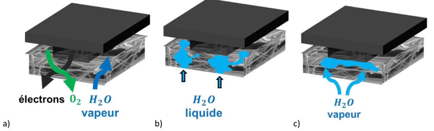
The goal of this thesis is to model the transport properties of GDL. The GDLs are crossed by gas, electron, heat and water flows. The transport properties of GDLs are often difficult to measure experimentally, due to their small thickness (300 μm). Figure 1.9 illustrates the various physical phenomena modeled and simulated in this document.
To allow these multiple transports, the GDLs are composed of a fluid phase and a solid phase, itself composed of several materials. The microstructure of GDL plays a key role in trade-offs between transports. It makes it possi-ble to explain the anisotropies of the effective transport properties and to explain the changes of effective prop-erties of the GDLs under compression. We take great care to develop simulation tools that are predictive of the effect of the microstructure.
a) b) c)
Figure 1.9 Diagram of transports in a GDL, for an in-situ fuel cell configuration. The GDL is inserted between a bipolar plate (in black) and a catalytic layer. a) diffusive transport of electrons or gases b) transport of water injected in liquid form into the GDL c) condensation of water coupled to a diffusive transport of water vapor.
The efforts made in this thesis to model physical phenomena and microstructures are justified first by the ex-pected advances in the modeling of the behavior of water in porous electrode materials. This topic is crucial to better understand water management in GDL, which has a significant effect on the loss of concentration in the fuel cell. A second justification for this effort is to develop computer tools to help design porous fuel cell materi-als.
Note that designing materials by simulation is impossible without prior work in physics and applied mathematics, as we conduct during this thesis. The predominant physical phenomena must first be understood and put into equations before being simulated. Experiments and models complement each other at this stage, to better un-derstand physical phenomena. Then, mathematical methods must be put in place to ensure the numerical pre-cision of the simulations and to manage the complexity resulting from the complexity of the geometries, and possibly couplings between physical phenomena. The work on the numerical precision of the simulations, in turn, allows us to acquire new information tu study physical phenomena, for example by making it possible to exploit models based on tomographic images.
1.2.2 Implemented approach
To better understand the effect of the microstructure of porous materials on transport, we are taking advantage of advances in imaging techniques that allow us to know precisely the microstructure of fuel cell porous materi-als. Chapter 2 provides information on the use of imaging techniques for porous materimateri-als. We focus in this paper on a material, the GDL, because we have images of their microstructure. In fact, X-ray tomography images are more readily available for GDLs than for other electrode materials because the resolution constraint is lower for GDLs. This GDL study is a first step in setting up the methodology and the tools for analyzing tomographic images and performing simulations on images. These tools allow the quantitative exploitation of tomographic images of porous materials and may in future be applied to other porous materials than the GDL.
We develop processing tools for tomographic images and physical simulation tools that work on 3D images. Fig-ure 1.10 and Appendix 9.1 provide a graphical overview of the various imaging and simulation tools used in this document. A first simulation tool used is an open source tool for direct simulation of diffusive transport on mi-crostructures. A second simulation tool used is a pore network simulation code that we have developed. On the
![Figure 2.6 Diagram of an X-ray tomography device. Taken from [Straubhaar2015].](https://thumb-eu.123doks.com/thumbv2/123doknet/3164306.90233/65.892.109.756.266.605/figure-diagram-x-ray-tomography-device-taken-straubhaar.webp)