Complete Flood Frequency Analysis in Abiod Watershed
1Biskra (Algeria)
23
S. BENAMEUR1, A. BENKHALED2, D.MERAGHNI1, F.CHEBANA*3, A. NECIR1 4
5
1Laboratory of Applied Mathematics, University of Biskra, Po Box 145, RP 07000 Biskra, Algeria
6
2Research Laboratory in Subterranean and Surface Hydraulics -LARHYSS, University of Biskra, Po Box 145,
7
RP 07000Biskra, Algeria 8
3INRS-ETE, University of Quebec, 490 rue de la Couronne, Québec, QC, Canada
9 10
*Corresponding author: [email protected] 11
November 2016 12
ABSTRACT 14
Extreme hydrological events, such as floods and droughts, are one of the natural disasters 15
that occur in several parts of the world. They are regarded as being the most costly natural 16
risks in terms of the disastrous consequences in human lives and in property damages. The 17
main objective of the present study is to estimate flood events of Abiod wadiat given return 18
periods at the gauge station of M’chouneche, located closely to the city of Biskra in a semi-19
arid region of Southern-East of Algeria. This is a problematic issue in several ways, because 20
of the existence of a dam to the downstream, including the field of the sedimentation and the 21
water leaks through the dam during floods. The considered data series is new. A complete 22
frequency analysis is performed on a series of observed daily average discharges, including 23
classical statistical tools as well as recent techniques. The obtained results show that the 24
Generalized Pareto distribution (GPD), for which the parameters were estimated by the 25
maximum likelihood (ML) method, describes the analyzed series better. This study also 26
indicates to the decision-makers the importance to continue monitoring data at this station. 27
Key words : Frequency analysis; Peaks-Over-threshold ; Generalized Pareto distribution 28
;Threshold selection ; Flood discharges ; Extremequantiles; Biskra ; Algeria. 29
Introduction 31
The study of floods is a subject which arouses more and more interest in the field of water 32
sciences. In spite of their low rainfall, the basins of the arid and semi-arid areas represent a 33
hydroclimatic context where the overland flows phenomena are significant and feed a network 34
of very active wadis. The activity of these wadis is far from being negligible from the flood in 35
terms of their frequency and intensity. One observes on these rivers exceptional flows which 36
sometimes, surprise by their magnitude[19]. The Abiod wadi, in the area of Biskra, is a very 37
representative river of these basins. Moreover, the existence of Foum El Gherza dam to the 38
downstream for the irrigation of the palm plantations makes the area more sensitive with regard 39
to the floods. The flood events of the years 1963, 1966, 1971, 1976 and 1989 remain engraved 40
in the memory of the inhabitants. The flood event of 11- 12th September 2009 was one of the 41
historic floods in the Zibans area[7]. It rains 80 mm in 24 hours, while the annual total of Biskra 42
city reaches 100 mm. The damage were 9790 palm trees, 164 flooded houses, 744 destroyed 43
greenhouses, 200 hectares of lost cultures. The last flooding at the time of this drafting paper 44
is that produced in October 29th 2011. All the populations living downstream of the Foum El 45
Gherza dam were evacuated. The floods mainly occur in September and October and especially 46
originate from exceptional storm events. 47
Describing and studying these situations could help in preventing or at least reducing severe 48
human and material losses. The strategy of prevention of flood risk should be founded on 49
various actions such as risk quantification. On this aspect, various methodological approaches 50
can contribute to this strategy, among which flood Frequency Analysis (FA). Frequency 51
analysis of extreme hydrological events, such as floods and droughts, is one of the privileged 52
tools by hydrologists for the estimation of such extreme events and their return periods. The 53
main objective of FA approach is the estimation of the probability of exceedance P X
xT
, 54called hydrological risk, of an event x corresponding to a return period T[16].This process is T
55
accomplished by fitting a probability distribution Fto large observations in a data set. Two 56
approaches were developed in the context of extreme value theory (EVT). The first one, usually 57
based on the generalized extreme value distribution (GEV), describes the limiting distribution 58
of a suitably normalized annual maximum (AM) and the second uses the generalized Pareto 59
distribution (GPD) to approximate the distribution of Peaks-Over-Threshold (POT). For more 60
details regarding this theory and its applications, the reader is referred to textbooks such as 61
Embrechts et al.[24],Reiss and Thomas[51], Beirlant et al.[6] and de Hann and Ferriera [18]. 62
Many FA models should be tested to determine the best fit probability distribution that describes 63
the hydrologic data at hand. Specific distributions are recommended in some countries, such as 64
the Log-normal (LN) distribution in China[10]. In the United States, the Log-Pearson type 3 65
distribution (LP3) has been, since 1967[44], the official model to which data from all 66
catchments are fitted for planning and insurance purposes. By contrast, the United Kingdom 67
endorsed the GEV distribution[45, 46]up until 1999.The official distribution in this country is 68
now the generalized logistic (GL), as for precipitation in the United States[59]. There are 69
several examples where a number of alternative models have been evaluated for a particular 70
country, for example Kenya[43], Bangladesh[35], Turkey[5] and Australia [58]. Nine 71
distributions were used with data from 45 unregulated streams in Turkey by Haktanir[26]who 72
concluded that two parameter Log-normal (LN2) and Gumbel distributions were superior to 73
other distributions. Recent research was conducted by Ellouze and Abida[23]in ten regions of
74
Tunisia. They found that the GEV and GL models provided better estimates of floods than any
75
of the conventional regression methods, generally used for Tunisian floods. Rasmussen et
76
al[50]reveals that the POT procedure is more advantageous than the AM in the case of short 77
records. Lang et al.[40] develop a set of comprehensive practice-oriented guidelines for the use
78
of the POT approach. Tanaka and Takara[55] has examined several indices to investigate how
to determine the number of upper extremes rainfall best for the POT approach.
80
In the Algerian hydrological context, during the last two decades many authors have used 81
several approaches to study the associated risks. Recently, Hebal and Remini[29]studied flood 82
data from 53 gauge stations in northern Algeria, between 1966 and 2008. They found that 50 %, 83
25 % and 22 %of the samples follow respectively the Gamma, Weibull and Halphen A 84
distributions. Bouanani [12]performed a regional flood FA in the Tafna catchments and 85
concluded that the AM flows fit better to asymmetric distributions such as LP3, Pearson 3 and 86
Gamma. The FA was also used in the sediment context by Benkhaled et al. [8]where the LN2 87
distribution was selected in the case of the same station considered in the present study, i.e. 88
M’chouneche gauge station on Abiod wadi. 89
To the best knowledge of the authors, apart from Benkhaled et al. [8], the flood FA approach 90
has not yet been performed on data collected at this station. The primary aim of this paper is to 91
perform a FA to the Abiod wadi flow data by the POT approach, based on GPD approximation 92
[30].In methodological terms, all the steps constituting FA are performed from data 93
examination to risk assessment including hypotheses testing and model selection. Due to the 94
high importance of the latter and its impacts, more recent techniques are employed to select the 95
appropriate distribution that fit better to the tail. A relatively large number of known 96
distributions fit well the center of the data whereas the focus in FA is on the distribution tail. 97
To this end, tail classification and specific graphical tools are employed, see El Adlouni et al. 98
[22] for more technical details. 99
The paper is organized as follows. In Section 2, the study area and the data set are briefly 100
described. Section 3 is devoted to the FA methodology. The results of the study are presented 101
and discussed in Section 4. Concluding remarks are reported in Section 5. 102
1. Study area and data 104
In this section, we present the region where the site of interest is located, followed by a 105
description of the available data. 106
1.1 Study Area
107
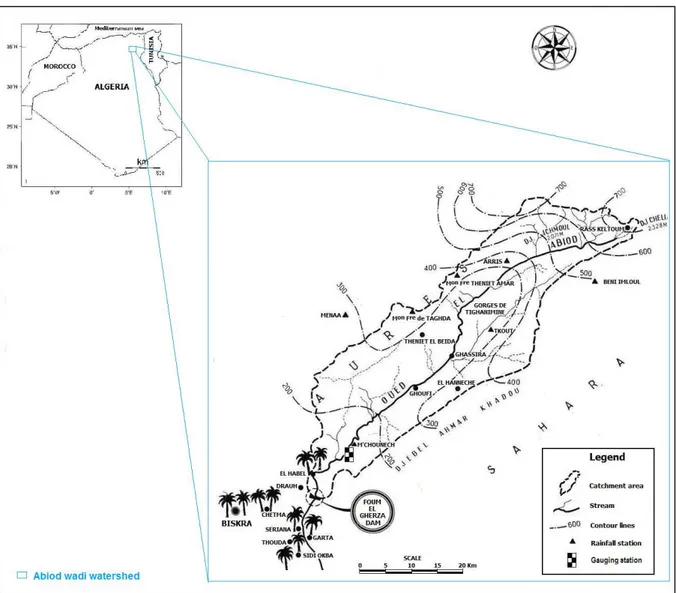
The Abiod wadi watershed, with an area of 1300 Km2, is located in the Aurès massif in the 108
southern east of Algeria in North Africa (Figure 1). It is part of the endorheic watershed Chott 109
Melghir. The wadi length is 85 km from its origin in the Chelia (2326 m high) and Ichemoul 110
(2100 m high) mountains. After crossing Tighanimine, the wadi gradually flows into the 111
canyons of Ghoufi and M’chouneche gorges, and then opens a path to the plain until the 112
Saharian gorge Foumel Gherza. The valley of the wadi is mainly composed of sedimentary 113
rocks, comprising alternating limestone, marl, soft sediments (sandstones, conglomerates) and 114
some evaporates (gypsum) dated of Paleogene. 115
The watershed is characterized by its asymmetry, a mountainous area in the north to over 2000m 116
(Chelia) and another low area in the south (El Habel 295 m). The relief is rugged with slopes 117
ranging between 12.5% and 25% for half of the area, and from 3% to 12.5% for another 40% 118
of the area. Land cover is a mix of rocky outcrops, highly eroded soil, sparse vegetation, a few 119
forests, crops, gardens and pastures [27]. In the orographic and hydrographic points of view, 120
Abiod wadi is characterized by two distinct climatic regions: the Aurès, where rainfall averages 121
450 mm/year, and the Sahara plain with mean rainfall 100-150 mm/year. The climate of Abiod 122
wadi watershed is thus semi-arid to arid. Along Abiod wadi to the Foum El Gherzadam there 123
are six rainfall stations, and one hydrometric station located 18 km upstream of the dam, as 124
shown in Figure 1, which was damaged during the floods of 1994-1995 and it is not operational 125
since. 126
The choice of this station was made on the basis of climatic context of the study area. It is the 127
only station on the studied basin and it is rather representative of the whole south-east region 128
in Algeria, which is arid to semi-arid.Also, the size of the series used shows the interest of the 129
FA application. 130
1.2 Data Description
131
The data set used in this study is provided by the National Agency of Hydraulics Resources 132
(ANRH) of Biskra and it is the first time to be considered and studied. It consists of the daily 133
average dischargesQ1, ,QN (with N = 8034), collected at the gauge station of M’chouneche 134
over 22 years from 1972 to 1994. 135
Note that the IACWD Bulletin 17B [1] suggests that at least 10 years of record are necessary 136
to warrant a statistical analysis. For instance, Tramblay et al. [57] used a minimum of 10 years 137
of daily data. The short data size can affect the choice of distributions, the quantile estimations, 138
particularly those corresponding to large return periods and the extent of confidence intervals. 139
The size of the used data in the present study is relatively large, to perform a FA, as in a number 140
of similar studies[15]. 141
2. Methodology 142
In this section, after defining the type of series to be analyzed, namely the POT series, we briefly 143
present the required elements to perform a hydrological FA. The latter is a statistical approach 144
of prediction commonly used in hydrology to relate the magnitude of extreme events to a 145
probability of their occurrence[16]. It allows, for the selected station, to estimate the flood 146
quantiles of given return periods. In general, FA involves four main steps: 147
(i) characterization of the data and determination of the usual statistical indicators, such as 148
the mean, the standard-deviation, the coefficients of skewness (Cs), kurtosis (Ck) and 149
variation (Cv)and detection of outliers, 150
(ii) checking the basic hypotheses of FA, i.e. homogeneity, stationarity and independence, 151
applicability on the studied data set, 152
(iii) fitting of probability distributions, estimation of the associated parameters and selection 153
of the best model to represent the data, and 154
(iv) risk assessment based on quantiles or return periods, [e.g. 11, 14, 26, 49]. 155
3.1. Peaks Over Threshold Series
156
The data to be extracted and then used in this approach consist in the observations that exceed 157
a selected relatively high thresholdu . Let Q represent the daily average discharge and denote
158
byN the number of discharges exceeding u . Then, the sample of excesses is defined as u
159
. . ; 1,
. j j j i i u E Q u s t Q u j N 160In this approach the selection of an appropriate threshold is crucial. This approach is useful and 161
has some advantages compared to the AM one, even though the latter is widely used. It is of 162
particular interest in situations where the AM could not perform well especially in situation 163
with little extreme data or the extracted extremes by AM cannot be considered as extremes in 164
a physical or hydrological meaning. 165
3.2.1.GPD Approximation
166
Statistically, the distribution of the POT series 1, ,
u N
E E ,can be determined by making use of 167
the GPD which is a cdfG , defined, for xS
,
:
0, if
and 0
0, /
if , 0168
by: 169
1/ , / 1 1 , 0, 1 x , 0, x G x e (1)where𝛾 ∈ 𝑅 and
0
are respectively shape and 170scale parameters[31]. 171
LetFu
x P Q u
x Qu
denote the excess cdf of Q over a given threshold u . Then, we 172have the following result: 173
,
0 lim sup 0, F F u u uq x q u F x G x (2) 174where q is the right end point of the cdf F F. This result, due to Balkema andde Haan[4] and 175
Pickands [48],is one of the most useful concepts in statistical methods for extremes. It says that 176
for large threshold u , the excess cdf F is likeley to be well approximated by a GPD. u 177
3.2.2.Threshold Selection
178
In order to obtain the asymptotic result in(2), the threshold u should be large enough which has 179
as a consequence a satisfactory GPD approximation. The choice of the threshold is a crucial 180
issue in the POT procedure. Indeed, selecting a threshold that is too low results in a large bias 181
in the estimation, whereas taking one that is too high yields a big variance[24, section 6.4 and 182
6.5]. Hence, a compromise between bias and variance is to be found. To this end, one can 183
minimize the asymptotic mean squared error, which is composed by the bias and variance. 184
Furthermore, several graphical procedures are available to selectu , such as the mean residual
185
life (MRL), threshold choice (TC) and dispersion index (DI) plots. On the other hand, the choice 186
of u can be based on physical considerations, e.g. by identifying the flood level of the river of 187
interest. For a survey of the main selection procedures, see e.g. the paper of Lang et al [40]. 188
3.2.Exploratory Data Analysis
The first step allows to check the data quality and to screen the data to avoid outlier effects. It 190
also permits to obtain prior information, e.g. the shape, regarding the distribution to be selected. 191
The presence of outliers in the data can have an important effect and causes difficulties when 192
fitting a distribution[3]especially on the distribution upper part. The Grubbs and Beck[25] 193
statistical test, based on the assumption of normality data, is designed to detect low and high 194
outliers. In the case where the original data are not normal, they should be appropriately 195
transformed. According to Section 1.8.3 in[49], this test is based on the following quantities: 196
exp , H n x xk s (3) 197
exp , L n x xk s (4) 198where xand s are respectively the mean and standard deviation of the natural logarithms of the
199
sample, and k is the Grubbs-Beck statistic tabulated for various sample sizes and significance n
200
levels by Grubbs and Beck [25]. For instance, at the 10% significance level, the following 201 approximation is used 202 1/4 1/2 3/4 .62201 6.28446 – 2.49835 0.491436 – 0.037911 , 3 n n n n k n (5) 203
where n is the sample size. 204
The observations greater than x are considered to be high outliers, while those less than H xL
205
are taken as low outliers. 206
3.3.Testing Independence, Stationarity and Homogeneity
207
Three basic assumptions are required to correctly apply FA of extreme hydrological events, 208
namely independence, stationarity and homogeneity of the data[11]. To verify these 209
assumptions, three tests are widely used in the literature. The Wald-Wolfowitz test is employed 210
for the independence, the homogeneity test of Wilcoxon is applied to check whether the data 211
come from the same distribution or not and the Mann-Kendall test allows to verify stationarity 212
of the data, i.e. the series does not present a trend over time. These three tests have the advantage 213
of being non-parametric and are widely used in hydrological FA. In other words, they do not 214
require any prior knowledge on the distribution of the data. 215
3.4.Parameter Estimation and Model Selection
216
The choice of the appropriate model is one of the most important issues in FA. In practice the 217
distribution of hydroclimatic series is not known. Using the fitted probability distribution, it is 218
possible to predict the probability of exceedance for a specified magnitude, i.e. quantile, or the 219
magnitude associated with a specific exceedance probability. To estimate the parameters 220
associated to the appropriate probability distribution, popular techniques are used in hydrology, 221
including the methods of Maximum Likelihood (ML)[e.g. 17, 46], Moments (MM) and 222
Probability Weighted Moments (PWM) [e.g. 13, 32]. The latter is equivalent to the L-moment 223
method which is widely used in hydrological FA[29]. 224
The choice of the adequate distribution is determined on the basis of numerous classical and 225
recent statistical tools, including graphical representations [34, 46] and goodness-of-fit tests 226
such as the tests of Pearson (Chi-squared, Chi2), Kolmogorov-Smirnov (KS), Cramer-von 227
Mises and the normality specific Shapiro-Wilk (SW) test. Due to the importance of the 228
distribution impact in FA, these tools should be exploited. This point is widely studied in the 229
literature [8, 20, 22, 28, 31, 38 and 47]. 230
Nonetheless, the decision procedures mentioned above are not perfectly suited for extreme 231
value distributions, because they are not sensitive enough to deviations in the tails. Several 232
transformations have been proposed to overcome the limitations of the aforementioned tests 233
[36, 39, 41]. In our application, where we focus on the upper tail of the distribution, we perform 234
the Anderson-Darling k-sample test (k=2) implemented in the adk package of the statistical 235
software R. This procedure is used to test the null hypothesis that k samples come from one 236
common continuous distribution. In our case, the first sample of size 42 is the considered POT 237
series and the second one consists in values generated from the GPD model. For more details 238
on this test, we refer to [53]. 239
The probability distributions that are appropriate for hydrology data are those with heavy tails. 240
A number of them are listed, e.g. in [37, 49, 52]. In order to select the appropriate distribution 241
among those which passed the goodness-of-fit tests, one or more criteria are required. To this 242
end, one can consider the Akaike and Bayesian information criterion (AIC, BIC) respectively 243
proposed by Akaike [2] and Schwartz [54]. They are given by: 244 2 ln 2 , AIC L k (6) 245
2ln
2 ln
BIC
L
k
m
(7) 246where L is the likelihood function, the number of parameters and mthe sample size. The best 247
fit is the one associated with the smallest criterion AIC or BIC values [20, 28, 49]. 248
3.5.Quantile Estimation
249
Once the appropriate distribution selected, the quantiles and return periods can be evaluated. 250
The quantile estimation for various recurrence intervals is the main goal in hydrological practice. 251
The notion of return period for hydrological extreme events is commonly used in FA, where 252
the objective is to obtain reliable estimates of the quantiles corresponding to given return 253
periods of scientific relevance or government standard requirements[49]. In the FA context the 254
uncertainty decreases with the sample size whereas it increases with the return period when 255
estimating quantiles. 256
In many environmental applications the sample size is rarely sufficient to enable good extreme 257
quantiles estimations. Usually, a quantile of return period T can be reliably estimated from a 258
data record of length n if T<n. However, in many cases, this condition is rarely satisfied –since 259
typically n<50 for hydrological applications based on annual data[31]. 260
3. Results and discussion 261
The application of the presented methodology in section 3 to the data described in section 2 262
leads to the following results, obtained by means of the packages stats, evir and POT of the 263
statistical software R [33] and also by using the HYFRAN-PLUS software[21]. 264
4.1.Exploratory Analysis and Outlier Detection
265
From Figure 2, it appears that the whole daily data series vary from a minimum value of0m3/s
266
corresponding to many dry days, to a maximum value of78.57m3/s recorded on September
267
21st, 1989. The average flow of0.39m3/s is a relatively low in comparison with other tributary
268
wadis of Chott Melghir like El Hai wadi and Djamorrah wadi [42]. The standard-deviation of 269
3
2.48m /s yields a coefficient of variation equal to 6.39 .The box-plot in Figure 3clearly 270
shows the existence of extreme values. Indeed, the median (0.10m3/s ) is close to both 25th 271
and 75th percentiles ( 3
0.04m /s and0.20m3/s ). In addition to this graphical consideration, the
272
values of skewness and kurtosis 3
(20.51m /s and 498.59m3/s respectively) eliminate the
273
Gaussian model. In particular the very large value of the kurtosis indicates longer and fatter 274
distribution tails, urging us to focus on heavy-tailed models 275
From Erreur ! Source du renvoi introuvable., we observehigh inter-annual and the short 276
sample size (resulting from selection AM) which leads to selecting low discharges during the 277
driest years whereas some interesting discharges were not selected during the years where 278
several floods have occurred. This explains the non-relevance of the AM approach for Abiod 279
wadi data analysis and suggests that the POT approach would be more appropriate, and would 280
lead to a more homogeneous sample of extreme discharges. This method starts with the 281
selection of a convenient threshold, then the consideration of the observations that exceed this 282
threshold. 283
In order to detect outliers, the quantities x and H x are found to 508.31 and 0.08 respectively. L
284
Since there is no value greater than x and nor less thanH x , we conclude that, at the significant L
285
level of 10 %, no outlier exist among the excesses. Since it is difficult to use the outlier detection 286
test with the analysis of extremes and due to the lack of regional weather data, the significance 287
level to 10% is considered. 288
4.1.1.Threshold Selection
289
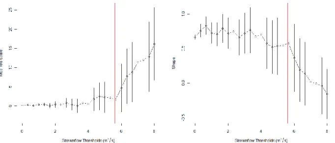
In this study, we adopt one of the available graphical tools, namely the TC-plot. From Figure 290
4we can choose a threshold valueu5.6m3/s, which results in an excess series of size 291
58.However, as recommended by many authors [9, 40, 56], this data set must be reduced in 292
order to avoid the effects of dependence. We eliminated the peaks being obviously part of the 293
same flood, and in order to keep the character of flood seasonality, we retain three peaks per 294
year over the recorded period. Thus, the length of the data series becomes 42. Figure 5shows 295
the distribution of these excesses and Table 1summarizes their elementary statistics. 296
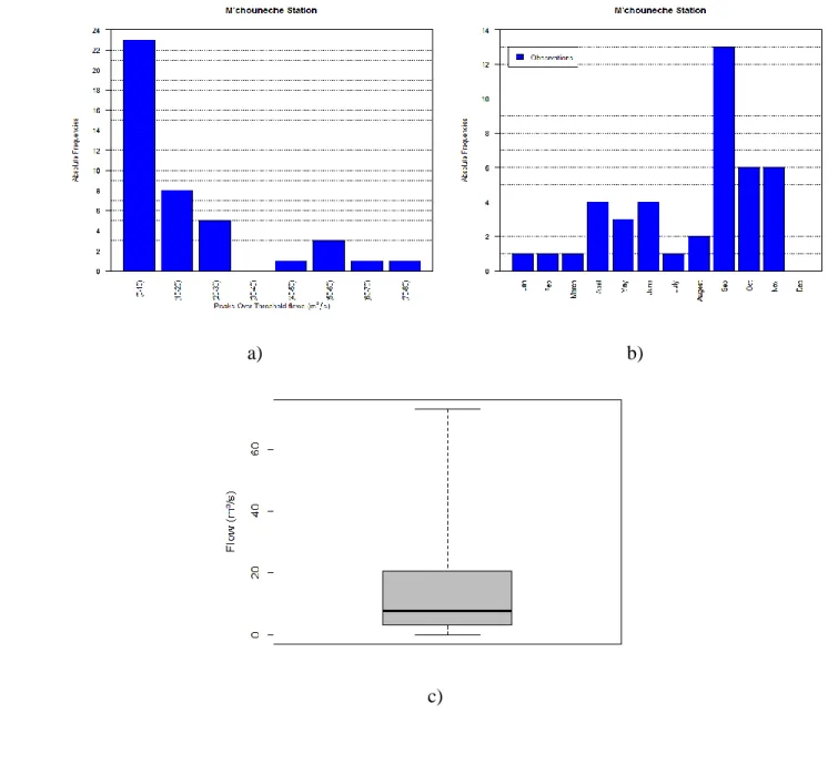
The positive skewness coefficient Cs=1.62 reveals that the data is right skewed relative to the 297
mean excess, as shown in Erreur ! Source du renvoi introuvable.a. In Figure 5a, the data are 298
arranged by classes, of length10 m3/s each, with the associated frequencies. It can be seen that 299
some values are more frequent than others and that the majority of excesses have a low value 300
varying between 0 and 10 m3/s. Erreur ! Source du renvoi introuvable.b, where the data are 301
arranged according to the months of appearance, shows that the peaks generally occur in the 302
fall season. 303
4.2.Testing the Basic FA Assumptions
304
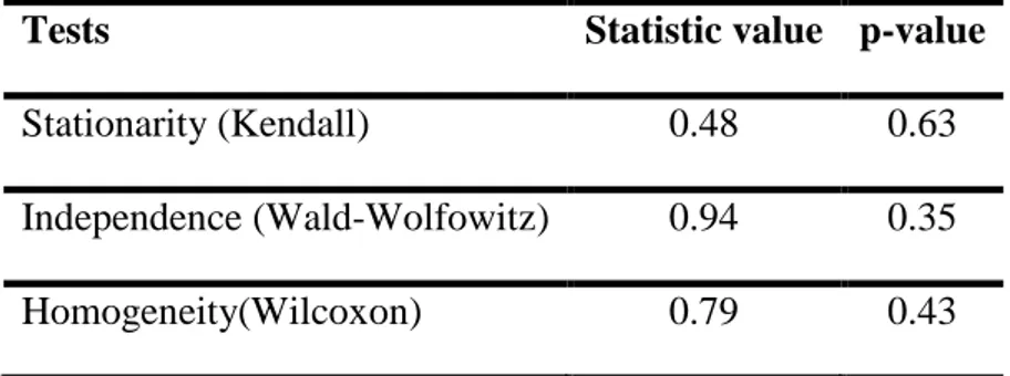
The results of the required hypothesis testing on the considered data are given in Table 2. 305
Applying Wilcoxon, Kendall and Walf-Wolfowitz tests respectively, we conclude that the 306
homogeneity, stationarity and independence of the excesses are accepted at any of standard 307
significance levels (1%, 5% and 10%).Note that for the homogeneity test, we split the data in 308
two sub-series 1972-1981 and 1982-1994 (any other subdivision led to the same conclusion). 309
The homogeneity can also be noted in Erreur ! Source du renvoi introuvable.a where there is only one 310
mode (the highest frequency). 311
4.3.Model Fitting
312
To fit a statistical distribution, we consider three commonly used estimation methods of the 313
GPD parameters (ML, MM, and PWM). Then we perform the Anderson-Darling test to check 314
the goodness-of-fit of the model. The results are summarized in Table 3. In view of the large P-315
values, we deduce that the GPD can be accepted as an appropriate model for the excess at any 316
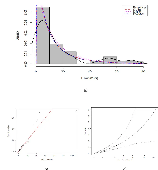
standard significance level (for instance 5%). 317
To discriminate between the obtained models, we use the AIC and BIC criteria. The last two 318
columns of Table 3as well as Figure 6bfavor the GPD of the ML fitting method. We illustrate 319
the goodness of fit of the excesses to this model in Erreur ! Source du renvoi introuvable.a. 320
Furthermore, this ML-based will be used for quantile estimation in the following section. 321
Note that the ML and PWM results are very similar whereas those of the MM results are slightly 322
different but remain in the same range. 323
4.4.Quantile Estimation
324
The estimation of extreme quantiles for different return periods should take into consideration 325
the record period and the right tail of the distribution. The formally gauged record represents a 326
relatively small sample of a much larger population of flood events. Thus, the extrapolation for 327
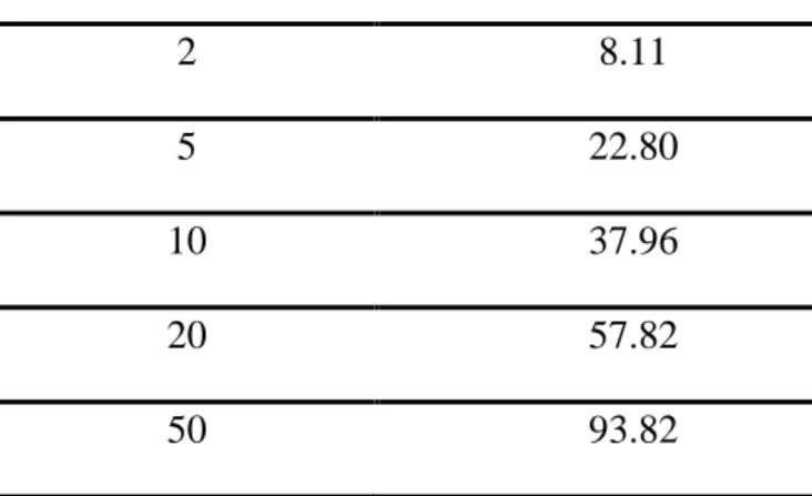
long return periods is less accurate. In the M’chouneche station only the following return 328
periods were considered for the estimation of quantiles: 2, 5, 10, 20 and 50 years as presented 329
in Table 4. The return period of the strongest streamflow in the 1972-1994 period, equal to 330
78.57 m3/s, is estimated by means of Pareto’s fitted model to be 30.62 years. 331
The confidence interval is a way to assess the uncertainty in the estimation of the distribution 332
parameters and quantiles. For the GPD, the confidence bounds are obtained through asymptotic 333
results [31]. In the present case-study, one can see from Erreur ! Source du renvoi 334
introuvable.c that the GPD agrees with the observations for return levels less than 30 but not 335
beyond even though they are all included in the confidence interval. This is probably due to the 336
small number of peaks over the chosen threshold. Therefore, it is important to consider this 337
distribution with care with return periods greater than 30 years. This point indicates the issue 338
of the quantity of the required data in this station for better estimation of high return periods. 339
4. Conclusions 340
The study of the Algerian wadis floods remains a quasi-unknown field as only some 341
very specific indications are given in the Algerian hydrological directories. Floods are one of 342
the basic features of a stream regime. The present study, which is the first one carried out in 343
southern east of Algeria with new data series, in the context of FA. Mean daily discharges data 344
recorded at the gauging station of M’chouneche in Abiod wadi, near Biskra, are available and 345
considered in the present study. Due to the high inter-annual variability of the data as well as 346
to the relatively short record length, the AM approach is not adapted to this analysis. Hence, in 347
this paper, we considered a more appropriate procedure, namely the POT method. 348
The purpose of this work is to provide a suitable model for the excesses over a chosen threshold. 349
This allows to estimate extreme flood events of given return periods. A complete FA was 350
applied including appropriate tools, commonly used in hydrology. The issue of threshold 351
selection was dealt by the means of a graphical tool. Several fitting methods have led to 352
different GPD models and according to the results, the ML-based distribution was adopted. 353
Because of the short record length, only return periods of 2, 5, 10, 20 and 50 years were 354
considered. It was found that most of extracted data corresponded to frequent events. In the 355
present case study, the GPD distribution provided good estimates of return periods less than 30 356
years but for higher values, the estimation is not acceptable and it is associated with high 357
uncertainty (large confidence interval). 358
As a conclusion, we should emphasis that, in addition to the quality of data and sample size, 359
the right choice of a GPD model heavily depends on the threshold. To improve the flood FA at 360
this site, future studies should focus on the importance of data monitoring. However, this 361
conclusion even it is not new in FA, it is important for the studied area where this is the first 362
time to be studied. It emphasis and confirms the importance of this issue, especially for local 363
government and decision makers. 364
Acknowledgments 365
The authors are thankful to the Editor and two reviewers for their constructive comments and 366
suggestions. The authors express their gratefulness to the financial support of Canada's 367
International Development Research Centre (IDRC). The data used in this study where 368
provided by the National Agency of Water Resource of Algeria (ANRH). 369
References 370
[1] (IACWD), I. C. o. W. D. (1982) Guidelines for determining flood flow frequency: Bulletin 371
17B (revised and corrected). Hydrol. Subcomm., Washington, D.C, 28. 372
[2] Akaike, H. (1974) A new look at the statistical model identification. Automatic Conrol, 373
IEEE, 19, 6, 716 - 723.
374
[3] Ashkar, F. and Ouarda, T. B. M. J. (1993) Robust estimators in hydrologic frequency 375
analysis. In: Engineering Hydrology (edited by C.Y Kuo) Am. Soc. Civ. Eng. New York, USA, 376
347-352. 377
[4] Balkema, A. A. and de Haan, L. (1974) Residual Lifetime at Great Age. Annals of 378
Probability, 2, 792-804.
379
[5] Bayazıt, M., Shaban, F. and Onoz, B. (1997) Generalized Extreme Value Distribution for 380
Flood Discharges. Turkish Journal of Engineering and Environmental Sciences, 21, 2, 69-73. 381
[6] Beirlant, J., Goegebeur, Y., Segers, J., Teugels, J., de Waal, D. and Ferro, C. (2004) 382
Statistics of Extremes: Theory and Applications. Wiley.
383
[7] Benazzouz, M. T. (2010) Flash floods in Algeria: impact and management. G-WADI 384
meeting. Flash Flood Risk Management Expert Group. Meeting Cairo 25-27 September 2010, 385
Egypt.
386
[8] Benkhaled, A., Higgins, H., Chebana, F. and Necir, A. (2014) Frequency analysis of annual 387
maximum suspended sediment concentrations in Abiod wadi, Biskra (Algeria). Hydrological 388
Processes,28,12, 3841-3854.
389
[9] Beran, M. A. and Nozdryn-Plotnicki, M. J. (1977) Estimation of low return period floods. 390
Hydrological Sciences Bulletin, 22, 2 , 275-282.
391
[10] Bobée, B. (1999) Extreme flood events valuation using frequency analysis. A critical 392
review. Houille Blanche, 54, 100-105.
393
[11] Bobée, B. and Ashkar, F. (1991) The gamma family and derived distributions applied in 394
hydrology. Water Resources Publications.
395
[12] Bouanani, A. (2005) Hydrologie, Transport solide et Modélisation. Etude de quelques sous 396
bassins de la Tafna. Université de Tlemcen.
397
[13] Chebana, F., Adlouni, S. and Bobée, B. (2010) Mixed estimation methods for Halphen 398
distributions with applications in extreme hydrologic events. Stochastic Environmental 399
Research and Risk Assessment, 24, 3, 359-376.
400
[14] Chebana, F. and Ouarda, T. B. M. J. (2011) Multivariate quantiles in hydrological 401
frequency analysis. Environmetrics, 22, 1, 63-78. 402
[15] Chebana, F., Ouarda, T. B. M. J., Bruneau, P., Barbet, M., El Adlouni, S. and Latraverse, 403
M. (2009) Multivariate homogeneity testing in a northern case study in the province of Quebec 404
Canada. Hydrological Processes, 23, 1690-1700. 405
[16] Chow, V. T., Maidment, D. R. and Mays, L. W. (1988) Applied Hydrology. McGraw-Hill, 406
New York, NY.
[17] Clarke, R. T. (1994) Fitting distributions. Chapter 4 Statistical modeling in hydrology. 408
Wiley, 39-85.
409
[18] de Haan, L. and Ferreira, A. (2006) Extreme Value Theory: An Introduction. Springer 410
Series in Operations Research and Financial Engineering. Boston. 411
412
[19] Dubief, J. (1953) Essai sur l’hydrologie superficielle au Sahara. GGA, Direction du Service 413
de la Colonisation et de l’Hydraulique, Service des Etudes Scientifiques, Alger, 457.
414
[20] Ehsanzadeh, E., El Adlouni, S. and Bobee, B. (2010)Frequency Analysis Incorporating a 415
Decision Support System for Hydroclimatic Variables. Journal of Hydrologic Engineering, 15, 416
11, 869-881. 417
[21] El Adlouni, S. and Bobée, B. (2010)Système d’aide à la decision pour l’estimation du 418
risqué hydrologique.IASH Publ, 340. 419
[22] El Adlouni, S., Bobée, B. and Ouarda, T. B. M. J. (2008) On the tails of extreme event 420
distributions in hydrology. Journal of Hydrology, 355, 16-33. 421
[23] Ellouze, M. and Abida, H. (2008) Regional Flood Frequency Analysis in Tunisia: 422
Identification of Regional Distributions. Water resources management, 22, 8, 943-957. 423
[24] Embrechts, P., Klüppelberg, C. and Mikosch, T. (1997) Modelling Extremal Events for 424
Insurance and Finance. Springer. 425
[25] Grubbs, F. E. and Beck, G. (1972)Extension of sample sizes and percentage points for 426
significance tests of outlying observations. Technometrics, 14, 847-854. 427
[26] Haktanir, T. (1992) Comparison of various flood frequency distributions using annual 428
flood peaks data of rivers in Anatolia. Journal of Hydrology, 136, 1-31. 429
[27] Hamel, A. (2009) Hydrogéologie des systèmes aquifères en pays montagneux à climat 430
semi-aride. Cas de la vallée d’Oued El Abiod (Aurès). Université, Mentouri : Constantine.
431
[28] Hebal, A. and Remini, B. (2011)Choix du modèle fréquentiel le plus adéquat à l’estimation 432
des valeurs extrêmes de crues (cas du nord de L’Algérie). Canadian Journal of Civil 433
Engineering, 38, 8, 881-892.
434
[29] Hosking, J. R. M. (1990) L-moments: analysis and estimation of distributions using linear 435
combinations of order statistics. Journal of the Royal Statistical Society, 52, 105–124. 436
[30] Hosking, J. R. M. and Wallis, J. R. (1987) Parameter and Quantile Estimation for the 437
Generalized Pareto Distribution. Technometrics 29, 339-349. 438
[31] Hosking, J. R. M. and Wallis, J. R. (1997) Regional frequency analysis; an approach based 439
on L-moments. Cambridge University Press, 224. 440
[32] Hosking, J. R. M., Wallis, J. R. and Wood, E. F. (1985) Estimation of the generalized 441
extreme value distribution by the method of probability-weighted moments. Technometrics, 442
257-261. 443
[33] Ihaka, R. and Gentleman, R. (1996) R: A Language for Data Analysis and Graphics. 444
Journal of Computational and Graphical Statistics, 5, 3, 299-314.
445
[34] Institute of Hydrology (IH). (1999) Flood Estimation Handbook. Wallingford, U.K, 1999. 446
[35] Karim, M. A. and Chowdhury, J. U. (1995) A comparison of four distributions used in 447
flood frequency analysis in Bangladesh. Hydrological Sciences Journal, 40, 1, 55-66. 448
[36] Khamis, H. J. (1997) The delta-corrected Kolmogorov-Smirnov test for the two-parameter 449
Weibull distribution. Journal of Applied Statistics, 24, 3, 301-318. 450
[37] Kite, G. W. (1988) Flood and Risk Analyses in Hydrology. Water Resources Publications, 451
Littleton, Colorado, USA, 187.
452
[38] Koutsoyiannis, D. (2003) On the appropriateness of the Gumbel distribution for odeling 453
extreme rainfall. In: Brath, A., Montanari, A., Toth, E. (Eds.), Hydrological Risk: Recent 454
Advances in Peak River Flow Modelling, Prediction and Realtime Forecasting. Assessment of
455
the Impacts of Land-use and Climate Changes. Editoriale Bios, Castrolibero, Bologna; 303–
456
319.
457
[39] Laio, F. (2004) Cramer-von Mises and Anderson-Darling goodness of fit tests for extreme 458
value distribution with unknown parameters. Water Resour. Res, W09308, 40. 459
[40] Lang, M., Ouarda, T. B. M. J. and Bobée, B. (1999) Towards operational guidelines for 460
over-threshold modeling. Journal of Hydrology, 225, 103-117. 461
[41] Liao, M. and Shimokawa, T. (1999) A new goodness-of-fit test for type-I extreme-value 462
and 2-parameter weibull distributions with estimated parameters. Journal of Statistical 463
Computation and Simulation, 64, 1, 23-48.
464
[42] Mebarki, A. (2005) Hydrologie des basins de l’Est Algérien. Université de Constantine. 465
[43] Mutua, F. M. (1994)The use of the Akaike Information Criterion in the identification of 466
an optimum flood frequency model. Hydrological Sciences Journal, 39, 3, 235-244. 467
[44] National Research Council (NRC) (1988) Estimating probabilities of extreme floods: 468
methods and recommended research. National Academy Press.
469
[45] Natural Environment Research Council (NERC) (1999) Flood Studies Report. Wallingford: 470
Institute of Hydrology, In five volumes.
471
[46] Natural Environment Research Council (NERC) (1975) Flood studies report. London, 1. 472
[47] Ouarda, T. B. M. J., Ashkar, F., Bensaid, E. and Hourani, I. (1994) Statistical distributions 473
used in hydrology. Transformations and asymptotic properties. University of Moncton.
474
[48] Pickands, J. (1975) Statistical inference using extreme order statistics. Annals of Statistics, 475
3, 1, 119-131. 476
[49] Rao, A. R. and Hamed, K. H. (2000) Flood Frequency Analysis. City. 477
[50] Rasmussen, P. F., Ashkar, F., Rosbjerg, D. and Bobée, B. (1994) The POT method for 478
flood estimation: a review. In: Hipel, K.W. (Ed.). Stochastic and Statistical Methods in 479
Hydrology and Environmental ngineering, Extreme Values: Floods and Droughts, Kluwer 480
Academic, Dordrecht. Water Science and Technology Library, 1, 15-26. 481
[51] Reiss, R. D. and Thomas, M. (2007) Statistical Analysis of Extreme Values: With 482
Applications to Insurance, Finance, Hydrology and Other Fields. Birkhauser Verlag GmbH.
483
[52] Salas, J. D. and Smith, R. (1980) Computer Programs of Distribution Functions in 484
Hydrology. Colorado State. University, Fort Collins, Colorado, USA. 485
[53] Scholz, F. W. and Stephens, M. A. (1987) K-sample Anderson-Darling Tests, Journal of 486
the American Statistical Association, Vol 82, No. 399, 918–924.
487
[54] Schwartz, G. (1978) Estimating the dimension of a model. The Annals of Statistics, 6, 461-488
464. 489
[55] Tanaka, S. and Takara, K. (2002) A study on threshold selection in POT analysis of 490
extreme floods. IAHS-AISH publication, 271. 491
[56] Todorovic, P. and Zelenhasic, E. (1970) A Stochastic Model for Flood Analysis. Water 492
Resources Research, 6, 6, 1641-1648.
493
[57] Tramblay, Y., St-Hilaire, A. and Ouarda, T. B. M. J. (2008) Frequency analysis of 494
maximum annual suspended sediment concentrations in North America. Hydrological Sciences 495
Journal, 53, 1, 236-252.
496
[58] Vogel, R. M., McMahon, T. A. and Chiew, F. H. S. (1993) Floodflow frequency model 497
selection in Australia. Journal of Hydrology, 146, 421-449. 498
[59] Willeke, G. E., Hosking, J. R., Wallis, J. R. and Guttman, N. B. (1995) The national 499
drought atlas (draft), IWR Rep US Army, Corps of Eng, 94-NDS-4. 500
List Of Tables 502
Table 1. Statistics summary of excess data set... 23 503
Table 2. Stationarity, independence and homogeneity tests results. ... 23 504
Table 3. GPD parameter estimation, Anderson-Darling goodness-of-fit test and 505
information criterion results. ... 24 506
Table 4. Estimated quantiles of excess flows from the ML-based GPD. ... 24 507
List Of Figures 508
Figure 1. Geographical location of the Abiod wadi watershed ... 25 509
Figure 2. Time series plot of the daily average discharge at M’chouneche station 510
covering the period 01/09/1972-31/08/1994. ... 26 511
Figure 3. Box plot of daily average discharge at M’chouneche station. ... 27 512
Figure 5. Distribution of excess series Ej at M’chouneche station a) Histogram by flow 513
classes b) Histogram by month c) boxplot. ... 28 514
Figure 6. Best fitted distributions of excess flows at M’chouneche station a) distributions 515
b) qqplot of ML-based GPD c) Return level plot (95% confidence interval) ... 29 516
517 518
Table 1. Statistics summary of excess data set. 519 520 Size 42 observations Minimum 0.02 m3/s Qu1(25th percentile) 3.36m3/s Median 7.83m3/s Average 15.72m3/s Qu2(75th percentile) 19.92m3/s Sd 19.70 m3/s Maximum 72.97m3/s Cs 1.62 Ck 4.48 521
Table 2.Stationarity, independence and homogeneity tests results. 522
Tests Statistic value p-value
Stationarity (Kendall) 0.48 0.63
Independence (Wald-Wolfowitz) 0.94 0.35
Homogeneity(Wilcoxon) 0.79 0.43
523 524
Table 3. GPD parameter estimation, Anderson-Darling goodness-of-fit test and 525
information criterion results. 526
Estimation method
Scale Shape Statistic value (Anderson-Darling)
p-value AIC BIC
ML 10.19 0.39 -0.55 0.49 315.68 326.63
MM 12.86 0.18 -0.83 0.58 316.61 327.56
PWM 10.10 0.36 -0.86 0.59 315.72 326.68
527
Table 4. Estimated quantiles of excess flows from the ML-based GPD. 528
Return period (years) Estimated quantile (m3/s)
2 8.11 5 22.80 10 37.96 20 57.82 50 93.82 529
530
Figure 1.Geographical location of the Abiod wadi watershed 531
534
Figure 3.Box plot of daily average discharge at M’chouneche station. 535
536
Figure 4.Graphical results of threshold selection applied for daily average discharge of 537
Abiod wadi at M’chouneche station (tc-plot), vertical line corresponding to the threshold. 538
539 540
541 a) b) 542 543 c) 544 545
Figure 5. Distribution of excess series at M’chouneche station a) Histogram by flow 546
classes b) Histogram by month c) boxplot. 547
549 a) 550 551 b) c) 552
Figure 6. Best fitted distributions of excess flows at M’chouneche station a) distributions 553
b) qq plot of ML-based GPD c) Return level plot (95% confidence interval) 554