Rule mining in maintenance: analysing large knowledge bases

Open Archive Toulouse Archive Ouverte (OATAO)

OATAO is an open access repository that collects the work of some Toulouse

researchers and makes it freely available over the web where possible.

This is

an author's

version published in:

https://oatao.univ-toulouse.fr/23612

Official URL :

https://doi.org/10.1016/j.cie.2018.11.011

To cite this version :

Any correspondence concerning this service should be sent to the repository administrator:

tech-oatao@listes-diff.inp-toulouse.fr

Grabot, Bernard Rule mining in maintenance: analysing large knowledge bases. ( In Press:

2018) Computers & Industrial Engineering. 1-15. ISSN 0360-8352

OATAO

Rule mining in maintenance: Analysing large knowledge bases

Bernard Grabot

INP-ENIT, University of Toulouse, 47, Avenue d'Azereix, BP 1629, F-65016 Tarbes Cedex, France

A R T I C L E I N F O

Keywords:

Association rule mining Maintenance Rule visualization Rule assessment

A B S T R A C T

Association rule mining is a very powerful tool for extracting knowledge from records contained in industrial databases. A difficulty is that the mining process may result in a huge set of rules that may be difficult to analyse. This problem is often addressed by an a priori filtering of the candidate rules, that does not allow the user to have access to all the potentially interesting knowledge. Another popular solution is visual mining, where visuali- zation techniques allow to browse through the rules. We suggest in this article a different approach generating a large number of rules as a first step, then drill-down the produced rule base using alternatively semantic analysis (based on a priori knowledge) and objective analysis (based on numerical characteristics of the rules). It will be shown on real industrial examples in the maintenance domain that UML Class Diagrams may provide an efficient support for subjective analysis, the practical management of the rules (display, sorting and filtering) being insured by a classical Spreadsheet.

1. Introduction

Companies are now computerised for a long time and have stored through years large amounts of data that could be used for generating

knowledge allowing to improve their performance (Harding, Shahbaz,

Srinivas, & Kusiak, 2006). The extraction of explicit knowledge from rough data is a major scientific and industrial challenge, that can be taken up by data mining techniques in a more or less automated way (Köksal, Batmaz, & Testik, 2011). Many tools can be used in that pur- pose, like decision trees, neural networks, genetic algorithms, k-means etc. The choice of a tool depends both on the expected type of knowl-

edge (patterns, clusters, association rules, etc.) (Choudhary, Harding, &

Tiwari, 2009) and on its potential use (clustering, diagnosis etc.) (Han and Kamber, 2006; Liao, Chu, & Hsiao, 2012). In this article, we focus on the structuration of knowledge in association rules, of the form IF (antecedents) THEN (conclusions), often considered as close to human

reasoning (Koskinen, 2012). The seminal works on association rule

mining have been performed on customer relationship (Agrawal,

Imielinski, & Swami, 1993; Agrawal & Srikant, 1994) but these tech- niques can also be useful on many aspects of manufacturing systems, like quality management, production planning, production control, etc. We consider here the maintenance domain, since decreasing main- tenance costs is nowadays a major industrial challenge, while the classical chain “symptoms-diagnosis-action-result” may help to struc- ture the data bases and the extracted knowledge. As a consequence, we shall here focus on extracting knowledge from maintenance records, even if the suggested approach can be transposed to many fields.

Many articles describe rule mining algorithms, but less address the difficult problem of the analysis of the generated knowledge base, that

can be very rich (Mansingh, Osei-Bryson, & Reichgelt, 2011; Potes Ruiz,

Kamsu-Foguem, & Grabot, 2014). Two main approaches are used in order to cope with this problem: decreasing the number of produced

rules in order to only generate “useful knowledge” (Gasmi, BenYahia,

Nguifo, & Slimani, 2005) or use different ways to visualize the rules in order to explore the knowledge base. We suggest here a different ap- proach: generate a large number of rules, without considering initially the genericity, robustness or type of generated rules, then explore the obtained (rich) rule base by performing alternatively a subjective se- mantic-based analysis (using already existing knowledge) and an ob- jective analysis (based on the numerical characteristics of the rules) of the knowledge base. In order to make the method transferrable to in- dustrial partners, we have chosen to do this using classical and simple tools, like UML and a spreadsheet. The suggested methodology is illu- strated on five real case studies.

The rest of the article is organized as follows: Section 2 defines the

context of industrial maintenance, summarizes the bases of rule mining and provides an overview of studies aimed at using data mining to

improve maintenance. Section 3 describes our methodological proposal

and the combination of tools suggested to deal with a large number of

rules. These proposals are applied to actual industrial cases in Section 4,

while the lessons learnt from this study are summarized in Section 5.

E-mail address: bernard.grabot@enit.fr. https //doi.org/10.1016/j.cie.2018.11.011

2. Context and state of the art

2.1. Industrial maintenance

According to European standards (EN6:1330, 2001, 2001), main-

tenance is defined as “the combination of all technical, administrative and managerial actions performed during the life cycle of an item in- tended to retain it in, or restore it to, a state in which it can perform the required function”. A distinction is usually made between curative maintenance, aimed at restoring the resource after failure, and pre- ventive maintenance, aimed at preventing the occurrence of defects. Preventive maintenance can be initiated at fixed i ntervals o r con- ditionally. The latter is often called predictive maintenance.

Maintaining an efficient an d co st-effective pro duction sys tem is becoming increasingly difficult as re sources be come mo re complex, particularly because of the profusion of technologies they carry (elec-

tronic, mechanical, hydraulic, pneumatic, computer, etc.) (Alsyouf,

2009). Many maintenance managers, supervisors and operators see a

lack of knowledge about the plant, its equipment and processes, as the main obstacle to implementing effective m aintenance procedures (Crespo Marquez and Gupta, 2006). It is therefore important to provide maintenance operators with effective decision support in their tasks of supervision, diagnosis, prognosis or in the choice of corrective or pre- ventive actions. To do this, it is tempting to consider the masses of data

accumulated over the years (Ben-Daya, Duffuaa, R aouf, K nezevic, &

Ait-Kadi, 2009). Indeed, most of the large companies use for main- tenance management dedicated information systems (Computer-Aided Maintenance Management Software - CMMS) or modules of their ERP (Enterprise Resource Planning) systems. T hese information systems store years of records on problems encountered and on the im- plemented solutions.

2.2. Data mining and maintenance

Data mining allows knowledge to be extracted from databases in an

automatic or semi-automatic way (Köksal et al., 2011). According to

Choudhary et al. (2009), however, it was initially rarely used for maintenance: in 2009, only 8% of studies using data mining in manu- facturing were oriented on maintenance. The strategic importance of preventive and predictive maintenance is now acknowledged by most of the companies, and as a consequence, data mining for maintenance

has experienced significant g rowth. Y oung, F ehskens, P ujara, Burger,

and Edwards (2010) propose to extract rules from a database in order to link failures, causes and corrective actions to be taken in the aero-

nautical industry. In the same sector, Baohui, Yuxin, and Zheng-Qing

(2011) seek to model the link between symptoms and corrective actions

by means of rules, while Maquee, Shojaie, and Mosaddar (2012) eval-

uate the effectiveness of maintenance actions carried out on a bus fleet.

Sammouri et al. (2012) are looking for rules combining alarms and

failures. (Bin and Wensheng, 2015) uses rule mining to help diagnose

high-speed trains. In (Djatna and Alitu, 2015) association rules are built

to link state of resources and required maintenance actions. In (Ruschel,

Alves Portela Santos, & de Freitas Rocha Loures, 2017), data mining is carried out on the time series of events generated by the process (“event logs”) to propose preventive maintenance actions. Deviations of pro-

duct quality are detected in real time in Glavar, Kemeny, Nemeth,

Matyas, and Monostori (2016) and linked to failures through correla-

tions identified by data mining. In Potes Ruiz et al. (2014), data mining

is used on reports of maintenance operations to generate rules linking data elements specified b y t he u ser ( e. g . s ymptoms a nd c ause). In

Accorsi, Manzini, Pascarella, Patella, and Sassi (2017), several classi- fication m ethods ( K-NN, d ecision t rees, r andom f orest, n eural net- works) and rule mining (Apriori algorithm) are used to analyse the machine behaviour before failures occur.

These studies have indeed shown promising results. Despite their diversity, they nevertheless share a number of similarities. First, they

seek to identify knowledge that can solve a specific problem (linking symptoms to causes, or causes to actions, or alarms to failures). Another approach could be to generate a large diversity of knowledge, then explore the obtained knowledge base for different purposes. This may possibly allow the emergence of unexpected but potentially useful knowledge. In the context of rule mining which will be ours, this raises the problem of managing a potentially very important number of rules. In this perspective, a second resemblance between the listed studies is that, as is often the case with data mining research, they place little emphasis on the post-processing of the knowledge base (with the ex-

ception of Accorsi et al. (2017)), and in particular on knowledge ana-

lysis and validation. These two points become essential if we accept to generate large rule bases linking any type of information.

In the following section, we summarize the basics of rule mining, then show how a combination of objective and subjective analysis techniques can make useful but sometimes unforeseen knowledge emerge.

2.3. Data mining basics

An experiment can be described by a set of descriptors. A main- tenance intervention can for instance be described by a date, the equipment concerned, one or several symptoms, a diagnosis and an action carried out. Recording such activity in a database D creates a “transaction”, composed of attributes (also called types or data types), each having a set of possible values. These values can be predetermined and selectable in a list (using a taxonomy of failures, symptoms or ac- tions for instance), or freely chosen by the person describing the transaction.

Data mining aims to uncover knowledge contained in large volumes

of data (Harding et al., 2006). Like statistical analysis, this knowledge

may denote associations between attribute values, but also between sets of values. An item is the value of an attribute. An itemset (also called a

pattern) is a set of items related to different attributes. A 1-itemset is an

itemset containing one item; a k-itemset contains k items.

The basic principle of data mining is that knowledge can be ob- tained by generalizing “frequent patterns”. To measure the frequency of an itemset, its support can be calculated, defined as the ratio between the number of transactions in which the itemset is present and the total number of transactions contained in the database. A minimum threshold is usually defined, above which an item will be considered as

frequent.

Different types of knowledge can be sought (Choudhary et al.,

2009), among which the best known are:

- Associations, gathering items that often occur at the same time. - Patterns, composed of item sequences staggered in time. - Classes, allowing to classify transactions according to patterns

known in advance.

- Clusters, also aiming at classification, but the groups being not known in advance.

- Predictive knowledge. The aim is to discover patterns leading to a prediction of the evolution of the entity observed in the transaction.

In association rule mining (Agrawal et al., 1993), knowledge is

structured in association rules, “IF X THEN Y”, denoted X → Y, where X

and Y are frequent itemsets. X is called the antecedent and Y the con- sequent of the rule but it is important to notice that a rule does not express a causal link between X and Y, but only the co-occurrence of these itemsets in transactions of the database. Let us notice that if many combinations of itemsets are frequent in the data base, there is a combinatorial explosion of the number of rules that may be difficult to handle. Association rules are well adapted to the maintenance problem, since they may show a possible correlation between symptoms, failures, causes, and actions that could be useful for improving the maintenance process.

= =

=

=

The oldest and best-known rule mining algorithm is Apriori (Agrawal and Srikant, 1994). This algorithm is executed in two steps: frequent itemsets are first identified, then rules are built by combining itemsets. The combination of itemsets during rule making is likely to

provoke a combinatorial explosion of the number of rules (Gasmi, Ben

Yahia, Mephu Nguifo, & Slimani, 2006). Many authors consider the generation of a large number of rules as an obstacle to the use of the

knowledge base (Agrawal et al., 1993; Djatna and Alitu, 2015; Gasmi

et al., 2006; Kotsiantis and Kanepoulos, 2006). In order to limit the number of rules, several solutions are possible, the basic idea being to define thresholds on numerical “measures of interest” supposed to ex- press the relevance of a rule. The most classical measures are the support (already used for finding frequent items) and the confidence.

The support sup of an association rule X → Y is the proportion of

transactions in D that contains both X and Y (Eq. (1)).

sup P(X Y) (number of transactions containing both X and Y)

/(total number of transactions) (1)

Confidence

P(X Y)/P(X) X Y Support

P(X Y) Lift _{P(X Y)/P(X)*P(Y)}

The confidence conf of the association rule X → Y is a measure of the reliability of the rule, determined by the percentage of transactions in D

containing X that also contain Y (Larose, 2005). Confidence is the

conditional probability P (Y|X) (Eq. (2)).

conf P(Y|X) P (X Y)/P(X)

(number of transactions containing both X and Y)

/(number of transactions containing X) (2)

Minimum values of the support (minsup) and confidence (minconf) can be defined: the rules that do not reach these thresholds are removed

by the mining algorithm (Agrawal et al., 1993). An a priori choice of

thresholds may seem arbitrary: some authors consider that it is more

natural to choose the number of desired rules (Garcia, Romero,

Ventura, & de Castro, 2009), once the rules have been produced and

ranked according to the chosen measure(s) (Scheffer, 2005). Another

strategy is to eliminate the “long rules”, containing many items in the IF

and THEN parts (Palanisamy, 2006; Scheffer, 2005).

Many other measures have been defined since the initial work of Agrawal et al., either for measuring the generality of a correlation (Laplace, chi-square statistics, correlation coefficients, entropy gain,

interest, conviction, etc. (Garcia et al., 2009)) or on the opposite its

specificity (peculiarity, diversity, novelty, surprisingness… (Geng and

Hamilton, 2006). Indeed, interesting knowledge may also come from rare associations, often called “outliers”.

More generally, for Geng and Hamilton (2006), several types of

measures can be distinguished to assess the value of a knowledge base: – objective measures, only based on the raw data, like support and

confidence,

– subjective measures, taking into account both the data and the user's

expectations. Potes Ruiz et al. (2014) suggest for instance to only

keep the rules consistent with a pattern defined using conceptual graphs.

– semantic-based measures, involving domain knowledge provided by the user. Because semantic measures involve domain knowledge provided by the user, some researchers consider them a special type

of subjective measures (Yao, Chen, & Yang, 2006).

On a medical application, Mansingh et al. (2011) control for in-

stance the extraction of the rules using both a domain ontology (al- lowing a subjective analysis) and an objective measure expressing the strength of a rule.

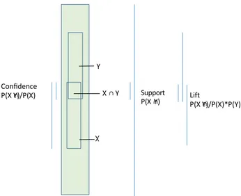
A semantic-based analysis of a rule may be facilitated by con- sidering the strength of the link between antecedent and consequent of the rule. In that purpose, another classical measure, the lift, may be of interest. The lift (or interest factor) can be obtained by dividing the

Fig. 1. Support, confidence and lift.

confidence of a rule by the unconditional probability of the consequent, or by dividing the support by the probability of the antecedent times the probability of the consequent:

lift( X Y) P(Y/X)/P(Y) support/(P(X). P(Y)) (3)

The interpretation of the lift is as follows: – if lift = 1, X and Y are independent, – if lift > 1: X and Y are positively correlated, – if lift < 1: X and Y are negatively correlated.

Fig. 1 summarizes the way the support, confidence and lift are calculated, emphasising their complementarity. The support does not take into account the frequencies of X and Y (only their intersection;

middle part of Fig. 1) while the confidence does not take into account

the frequency of Y (left part of Fig. 1). Tan, Steinbach, and Kumar

(2006) consider for instance that high confidence rules can be mis- leading, because the confidence measure ignores the support of the itemset appearing in the rule consequent. This is done in the lift (right part of the figure). Although classical, these three measures allow to give a rather comprehensive view on a produced rule within its context. Since our objective is more on the methodology than on the measures themselves, we have adopted these classical measures for our study.

Very often, (with the notable exception of Mansingh et al. (2011)),

objective evaluation is performed first, since it can easily be embedded in the mining algorithms, whereas semantic and subjective evaluation are performed on the remaining set of rules. As a consequence, rules that do not meet the thresholds during the objective evaluation phase are usually not considered by the experts of the field. On the opposite, we suggest to accept the possibility that many rules are created for accessing a wide variety of knowledge. We shall see in next section how a large set of rules can be managed through visualization techniques.

2.4. Visualizing association rules

Based on the observation that the analysis of many association rules

may be difficult (Hahsler and Chelluboina, 2015), some authors suggest

to address the analysis of large sets of rules through visualization

techniques (see surveys in Bruzzese and Davino (2008) or Hahsler et al.

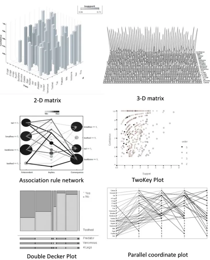
(2015)). Without claiming to be exhaustive (especially since these re- presentations have been object of many variants), we can list:

– two-dimensional matrices: the antecedent items are positioned on one axis and the consequent items on the other. The height and colour of

Y n n n _n X

n

n

•

Fig. 2. Visualization of association rules (Bruzzese & Davino, 2008).

a bar represent the support and confidence. These techniques hardly allow to represent many-to-one relationships.

– 3D-visualization: the rows of a matrix represent the items while the columns represent the rules. Bars with different heights visualize the antecedent and consequent parts while other bars represent the support and confidence of each rule.

– Association rule networks: each node represents an item, and the edges represent associations between items. The support and con- fidence are represented by the colour and width of the arrows. – TwoKey plot: the x-axis and y-axis represent respectively the support

and confidence; a rule is represented by a point on the graph. – Mosaic plots and Double decker plots, representing a rule and its

....

_

1r

ooe,

su~

on

1

2-D matrix

bfe-.>N:S-I.

__

,

QJ•or 1.

Association

rule

network

-..__

_{,___}

Double

Decker

Plot

Yes • No Toothed Predator Venomous 4 Legs

••

•

"

i

~

••

3-D matrix

- •no.a--.. _o0 00 •

.

f 0

di'

~··

~,

4 • 0

,

r

o,;.

0 <I>

•

•

I'..

..

00 ₀ 0 0

z..

$ 0 0 • ., I.-,. 0 ₀ 0 • • ..., • • fir 0 0

•

~ 00 0 • •

.

_{.. 8} 0

•

•

~ _~

.

0 0Q) ₀ o,ac, o.

~·

0 0 0 0

.

5

-

·

.

'

00 0 o. • 0 0

•

•

-

o'o ,fo

•

3 0 ₂

•

Suppoc

TwoKey

Plot

Parallel coordinate plot

V

-=-

,_

-

=..

_...

,

..

,...,

"·""

...

"'

--

-related rules by bar graphs.

– in Parallel coordinate plots, items are in lines, a rule being re- presented by joining antecedents by arrows and consequents by lines.

Examples of these visualizations, provided in Bruzzese and Davino

(2008), are shown in Fig. 2.

Let us notice that the visualization methods based on the items may be difficult to handle when many items are present in the rules, in re- lation with the combinatorial explosion already discussed. When the number of rules is important, a factorial method may help to synthetize

the information stored in the rules (Bruzzese & Davino, 2008) with

some loss of information. The result may be represented on factorial planes for items, rules, or joint representation.

These methods may indeed allow to represent large number of rules (several hundreds to several thousand) but the TwoKey plot is the easier tool for taking into account hundreds of thousands of rules, which is the order of magnitude that we shall deal with.

3. Suggested method

A preliminary proposal was made in Grabot (2017): (i) extracting as

much knowledge as possible from maintenance reports, (ii) display the rules obtained in a spreadsheet and (iii) explore the obtained rule base using the spreadsheet filters, by formulating hypotheses on potentially interesting knowledge, with the support of a class model of the data- base. This method proved to be promising on the basis of initial ex- periments, allowing in particular to efficiently manage hundreds of thousands of rules using a standard spreadsheet. However, more ex- tensive tests have shown that very different types of knowledge bases can be obtained. An objective analysis based on a graphical re- presentation of the rules can effectively complement this first semantic analysis.

3.1. Knowledge base generation

Numerous open source or commercial software programs allow the use of data mining tools on an existing database, including the R lan- guage that offers a very complete environment of statistical and gra-

phical processing.1 _{For our part, we have chosen to encapsulate data}

mining algorithms provided by Philippe Fournier-Viger2 _{in in-house}

developments for reasons of competence and flexibility, but this choice does not condition the use of the method.

Our objective is to facilitate the post-processing of the resulting rule base, not to propose a particular algorithm for extracting the rules. We

have therefore chosen the most classic algorithm, Apriori (Agrawal

et al., 1993), for the extraction of rules, as well as classical measures (support, confidence and lift) for the objective evaluation of the rules. Creating the rule base requires several steps:

Creation of the database: In order to have files that are easy to

manipulate in any environment, we have worked on csv files coming from Excel exports from the databases of the companies that provided

the data for tests. All the data bases analysed in Section 4 are extrac-

tions from the SAP ECC Maintenance module, which is understandable since SAP ECC is the ERP most often encountered in large companies.

Data cleaning: Preparing the data for a data mining process is re-

cognised as a difficult and long-lasting task. A structured process for

data-cleaning is for instance suggested in Mansingh, Osei-Bryson, Rao,

and McNaughton (2016). As a first step, some attributes can be re- moved without loss of information: for instance, the reference number of the manufacturing order aiming at identifying it in a unique way can obviously not be object of any generalisation. Other attributes that

1 _{https //www.r-project.org/.}

2 _{http //www.philippe-fournier-viger.com/spmf/index.php.}

make a transaction too specific should also be pre-processed: for in- stance, several databases mention several dates for each maintenance activity (planned, realized, etc.). Such information can hardly be gen- eralized, since few transactions concern the same day. As a con- sequence, the dates have been grouped by periods for our experiments. In that purpose, a simple program was developed allowing to group dates by week, fortnight or month, depending on the number of transactions per period.

As a third step, specific attention must be paid to text fields filled by the actors in a free manner, like the description of failures or causes for some companies. Indeed, many expressions can be used to describe the same observations (not mentioning spelling errors). Such fields should obviously be homogenized to allow generalisation. This is in practice only possible in a manual way, and so on a limited number of trans-

actions, if advanced text mining algorithms are not used (see (Arif-Uz-

Saman, Cholette, Ma, & Karim, 2016) for an example of the use of text mining on the maintenance domain). During this study, some fields, like the symptoms for instance, have been homogenized using taxo- nomies, but it has only been done on the small databases. On the largest databases, the text fields have been removed in order to simplify the first tests, described hereafter.

Extraction of the rules base: As stated in Section 2, the Apriori

algorithm first looks for frequent itemsets in relation to a minimum support. In order to generate as many rules as possible, we propose to set the three thresholds on support, confidence and lift measurements at values low enough to generate the highest number of rules that can be displayed and manipulated by a spreadsheet. In practice, this number depends not only on the spreadsheet but also on the RAM of the com- puter used. With a conventional 8 GB memory computer, the limit of the number of rules that can be displayed is below the million for Excel, and is even higher with OpenOffice. Filters are then applied to the different attributes (columns in the spreadsheet).

3.2. Result analysis

As shown in Section 2, most studies published on rule mining in

maintenance have a specific objective: to link symptoms to causes or causes to actions for example. Combined with the choice of fairly high thresholds for the measures of interest, the selection of the corre- sponding attributes makes it possible to drastically limit the number of rules produced, so the number of rules to assess. In our case, it is ne- cessary to provide a framework for the subsequent analysis of the generated rules. We suggest to combine objective analysis (related to the measures of interest) and subjective analysis (related to the analyst's interest and to prior knowledge) in that purpose. To do this, we propose

the approach summarized in Fig. 3 using the SADT syntax, based on the

idea of using only simple tools.

Ontologies aiming at describing the whole domain of maintenance

have already been suggested (see for instance (Karray, Chebel-Morello,

& Zerhouni, 2011)). We only need here a simple reference model of the

record of a maintenance order. We have therefore proposed in Grabot

(2017) to use a UML class model (Fowler, 2004) for providing such simple reference model in order to facilitate subjective analysis (activity

(S) in Fig. 3). Fig. 4 shows this basic model. This class diagram can be

used as a “map” for choosing possible “paths” between data using the relationships between attributes and their cardinalities. For instance,

the diagram of Fig. 4 suggests that there could exist associations be-

tween symptoms, failures and causes, or between maintenance orders, failures and equipments. Considering the cardinalities is of great in- terest in that purpose. For instance, the cardinality “*/*” between failure and symptom suggests (i) that the same symptom can be asso- ciated to different failures, (ii) that the same failure can result in dif- ferent symptoms. It is easy to check this assumption using the filters on the itemsets of the rule: it is enough to select a failure in the antecedent part of a rule, and to check whether several symptoms appear in the filter of the consequent part of the rule. This helps to check whether the

Fig. 3. Suggested methodology.

Fig. 4. Basic model of a maintenance order (Grabot, 2017).

theoretical view on the system is consistent with the operational reality of the process.

Since the databases that we will consider in the case studies all come from the same ERP (SAP ECC), one might expect a single reference model to be sufficient. This is not the case: the first reason is that SAP ECC has pre-set versions for a large number of industrial areas. The maintenance module of the “Aerospace and Defence” version, dedicated to discrete manufacturing, is for instance very different from the one of the “Pharmaceuticals” version, oriented towards continuous processes. The second reason is that the stored attributes and the database ex- tractions can be customized to specific requirements, which has been done by all the analysed companies. Starting from a standard class

model (Fig. 4) positioning the classical concepts in maintenance man-

agement (mainly: the maintenance order describing the equipment, symptoms, the diagnosed cause, and the action carried out), it will thus be required to produce the real model used in each company, which can be significantly different. This model will make it possible to formulate

hypotheses of correlation between attributes ((C) in Fig. 3) allowing to

define sequences of use of the spreadsheet filters. As illustrated in

Section 4, trying to find associations between two concepts using the

class model of Fig. 4 is rather easy: it is enough to consider two concepts

linked by a relation and to look in the spreadsheet whether values of the two items can be respectively found in the IF and THEN part of some rules. Extending the reasoning to more than two concepts is a bit more difficult because the items can be split in different manners in the two parts of the rules, but it can nevertheless be done without major pro-

blem, even if, for better clarity, the examples of Section 4 focus on two

items.

Our initial tests have shown that this “local” approach, guided by the analyst's prior knowledge, rarely leads to unexpected knowledge, that may be the most interesting. We therefore suggest that this sub- jective analysis could be flexibly combined with a more comprehensive objective analysis based on measures of interest. This should make it possible to identify groups of potentially interesting rules according to what the user is looking for. We propose for that a two-stage approach

that will be detailed on the case studies in Section 4:

- The knowledge base is firstly mapped by means of two main gra- phical tools visualizing the distribution density of the rules ac- cording to the different measures of interest, and the links between

distributio Type of _aim

Knowledge

---,

base? T

Objective Zones of

analysis ₀ zones

..

interest ₂ attributes

•

rule base Tableau Filtering rule~

F

Subjective Spreal:isheet

Correlation?

analysis

_s

class C attributes

model UML 8 _Operator -type -serial number -name 1

.1

.

1

1

8 _Equipment 8 Failure 8 Maintenance Order

1 ₁

-reference -description • reference

--;- -duration

-description

l

· type (C/P)

-criticality • description

-location 8 _Symptom -planned on:

/1\ _-type • realized on:

-description • created on:

)

8 _System -cost

l

-reference

-description 8 Cause 13 Action

-type -type

measures of interest (confidence as a function of support and lift as a

function of trust) ((C) in Fig. 3).

- After analysing the characteristics of the knowledge base ((T) in

Fig. 3), it is possible to identify areas of interest in the knowledge base (Z), the choice of which defines the objectives of the analysis (looking for generic knowledge or rare knowledge, for example). The attribute selection, which is the result of the objective and subjective analyses, will allow to manage the spreadsheet filters for selecting potentially interesting rules (F).

As it will be shown in Section 4, it may be useful to perform ob-

jective and subjective analysis alternatively in order to explore the data base (denoted by a feedback loop between activity (F) and activities (O)

and (S) in Fig. 4).

4. Case studies

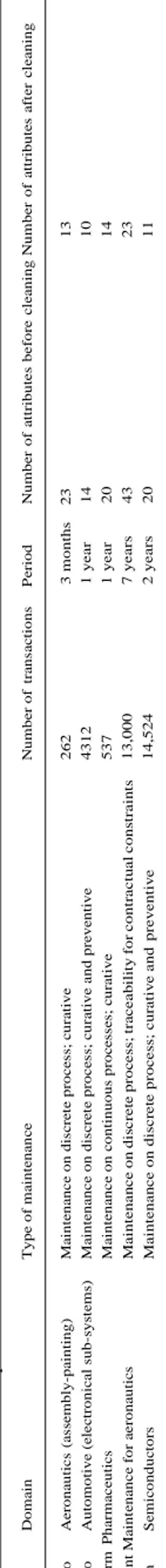
Five companies (of which the names have been changed) have ac-

cepted to provide real data for testing the method. Table 1 summarizes

the sector in which the companies operate and the main characteristics of the provided data bases. Let us notice that the provided files are extractions of the main database, and only contain the attributes chosen for the tests by the company.

Section 4.1 gives some details on the data cleaning of the data bases

used for the tests. As explained in Section 2, the rules are then gener-

ated using a standard Apriori algorithm, used with low thresholds on

the measures of interest (Section 4.2). For analysing the obtained rule

base, the user may look for rules having given characteristics (generic rules or exceptions; robust rules etc.) or may perform some hypothesis on correlations between attributes, then try to validate them. In the first

case, the analysis should begin by an objective analysis ((O) in Fig. 3;

see Sections 4.4 and 4.5), in the second case by a subjective analysis ((S) in Fig. 3; see Section 4.6).

4.1. Data cleaning

Only a basic data cleaning process was performed. Basically, the text fields were replaced by discrete sets of values using taxonomies suggested by the maintenance experts in the small data bases. For in- stances, “free” sentences describing symptoms were replaced by a type of symptom taken from a standard list. Since performing manually this operation is highly time consuming, it was decided to conduct the first tests on the large databases after removing all the text fields.

Since our algorithm replaces an empty content by the content “EMPTY”, empty fields were processed as a specific value of the con-

sidered attributes. As shown in Section 4, the result is that empty fields

are involved in many association rules, creating unexpected knowledge on the way the information was filled.

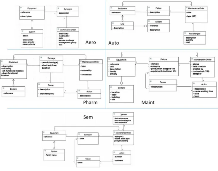
4.2. UML class diagrams

The first step is to build the UML class diagrams that will be used for

activity (S) of Fig. 3. Fig. 5 shows the class diagrams of the maintenance

data base in the five enterprises. For Aero, a rather simple model can be noticed, directly connecting a work order to a symptom and an equipment. The failure is not distinguished from its symptoms. The attributes removed during the cleaning phase essentially relate to planned and real action dates.

For Auto, the model is centred on a failure, in which a maintenance action is assimilated to a part change. Again, failure and symptom are not formally distinguished.

For Pharm, Maint and Sem, more standard models distinguish failure (called damage by Pharm), cause, action and maintenance order. It should be noticed that Maint being a company providing a main- tenance service, many attributes are intended to justify that the con- ditions of the contract are met. For these tests, we simplified the data

Tab le 1 M a in c h ar a c te ri st ics o f t h e c o m p an ie s a n d o f t h ei r d at a b as es . Do m ai n Aer o Aer o n au ti c s (as sem b ly -pa int ing) Au to A ut om ot ive ( e le c tr oni c a l sub -s y st e m s) P h ar m P h ar m ac eu ti cs M ai n t M ai n ten an c e fo r ae ro n au ti cs S em S e m ic onduc tor s T y p e o f m ai n ten an ce M ai n ten an c e o n d is cr et e p ro c es s; cu rat iv e M ai n ten an c e o n d is cr et e p ro c es s; cu rat ive a nd pr e ve nt ive M a int e na nc e on c ont inuous pr oc e ss e s; c ur a ti ve M ai n ten an ce on d is cr et e proc e s s ; tr a ceab il it y for co n tr act u al co n s tr ai n ts M ai n ten an ce o n d is cr et e p ro ces s ; cu rat iv e an d pre ve nt iv e N um be r of t ran s act io n s P er io d Nu m b er of a ttr ib u te s b e fo re cl ean in g Nu m b er of a ttr ib u te s af ter cl ean in g 262 4312 537 13,000 14,524 3 m ont hs 23 1 y ear 14 1 y ear 20 7 ye a rs 43 2 ye a rs 20 13 10 14 23 11

Fig. 5. Class diagrams.

base by removing a significant number of dates (date of failure, inter- vention data, date of temporary repair, date of return to a nominal state, etc.), which could also be analysed.

4.3. Rules extraction

Several tests have been conducted in order to extract a rich and multipurpose knowledge base. For that, the minsup and minconf have been set to very low values (for generating both generic and rare rules), while the minlift has been set to 0, in order to allow the generation of rules involving attributes of any types of correlation. The choice of the thresholds, and as a consequence the number of rules, was limited ei- ther by the memory used by the rule mining software, or by the

Table 2 Mining the rules.

possibilities of the spreadsheets used to display the rules and to act on them through scrolls and filters. The set-ups of the mining experiments

so that the obtained rule base are detailed in Table 2, were “Items” is

the number of different values of attributes found in the data base. Let us note for instance that for the set up (minsup = 1, minconf = 1, minlift = 0) for the Aero database, 2 601 506 rules are generated by the data mining software and stored in a text file without problem, but Excel cannot open the file, while LibreOffice “only” opens the first 1 048 576 rules. In any case, the problem is not only to open the file but also to manipulate the rules, which is why we have in each case gen- erated less than 1 million rules.

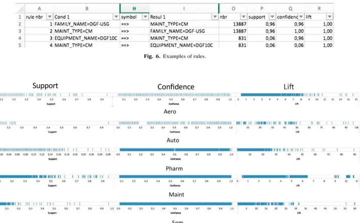
Examples of rules displayed by the spreadsheet are shown in Fig. 6

(here rules with only one antecedent and one consequent). There is one

rule per line in Fig. 6, the field “Cond1″ denoting the IF part of the rule

and ”Resul1″ the THEN part. “nbr” denotes the number of transactions on which the rule is based (the support also provides this information as a ratio) while the support, confidence and lift are the one of each rule.

Attributes Transactions Items Frequent itemsets

Minsup, minconf, minlift

Number

of rules 4.4. Characterisation of the rule bases

Let us consider steps (O) and (T) of Fig. 3. A first point is to de-

Aero 13 262 446 35,997 5 5 0 131548

Auto 10 4312 5284 1354 1 1 0 12260

Pharm 14 537 2148 4668 1 1 0 103648

Maint 23 13,000 12,724 10,656 8 8 0 645348

ST 11 14,524 2447 4663 1 1 0 66582

termine the objective of the analysis, i.e. whether we shall mainly look for generic or specific rules (outliers). In that purpose, it is interesting to first consider the distribution of the rules according to their measures of

interest (see Fig. 7). Let us remind that the support gives the percentage

of transactions expressed by a rule, the confidence whether a rule is

E

_,,...

_S,mo"""

.

,.,.,.P'IN

· delerlptlon • dncrlptlon -Mainten.anc. Ordlf

-

-enterad by • •tstut •trlOdffle<tl)y

.

....

•dacrlp(Jon • Mn"ice k, charge

Aero

•ccdep,ia,lty - ,nanagen'll'nt ,group

-dffcr.p,to,lty •ttlll •dHeripUon · crltlc•llty . dosc•ptlon(typo) ,_ _ _ __, · lhotl

.rl

(f,_I . <!oration > ' - - - I.typo • ,..t, tul"ldlONl roc.t4on • dncr.functional lo<ollon

·--

"

-dHcriptlor, Causo • short ,en

1,,..,

· entti'1d by •crutedon -dHcriptlon

Pharm

Sem

Uno • OHetlPUon

Auto

I

·

IB EQJJlpmen1 - reference • unit •dHcripllOn -family -crltlclty

6

1,i _Sy,tem • locatlon ·code • bulldlng •llto

·

--

Maln1enanc. Ordtt'

·

•lypO

-

(CIP) System PMCIW>ged

--•-•QU,lntlty ·COOi

.

]

.,

_{Failure I} O Mai'ltienar'l09: Order

'

•domain

,,---

• status

•• calOjlory • date creat~

• production alopped YIN ·C:rNledby

re • equipment 1hutdown YIN • • eontraetual category (YIN)

'I,

I

"'

Cause

I

_la

Ac1lon

y •dHcriptlot,

I

.

• caute

""""?I'°"

Wlhlng time

· load ·INm

Fig. 6. Examples of rules.

Support

Confidence

Sem

Fig. 7. Characterisation of the rule bases.

“robust” or not (the antecedent and consequent are often present at the same time), while the lift allows to analyse more precisely the link between antecedent and consequent (negative correlation; in- dependence or positive correlation).

Let us remind that lift = P(X ∩ Y)/P(X)*P(Y). If X and Y always

appear at the same time, P(X)=P(Y)=P(X ∩ Y), so lift = 1/P(X)=1/P

(Y). The lift is therefore maximum when X and Y always occur at the same time, and are rare. This means that high values of the lift denote rare events: the so-called “outliers” that can easily go unnoticed by traditional techniques filtering the rules according to the support. This can be easily checked on the rule bases: if only the rules of sup- port > 0.3 are selected, all the displayed rules have lifts and con- fidence around 1, while all the rules with high lift have a support in- ferior to 0.3.

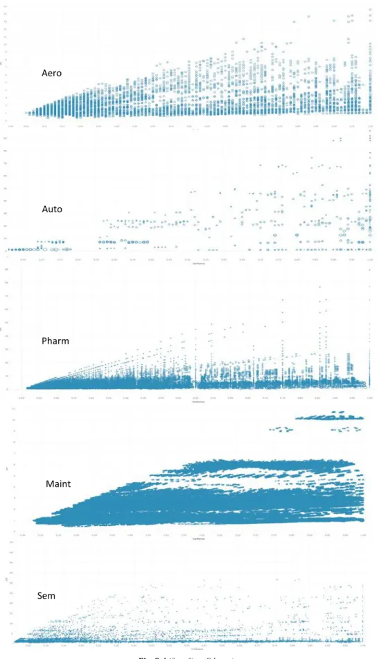
It can for instance be seen in Fig. 7 that all the rules bases have a

relatively well distributed confidence (i.e. rules of any support can be found in the rule base, i.e. rules with all possible degrees of genericity/

specificity). Nevertheless, Fig. 7 allows to define what is promising for

each rule base:

- Auto is mainly composed of rules of low support (rare knowledge) but the distribution of confidence is regular, meaning that robust knowledge should be present. Moreover, the maximum lift being rather high (100) with a pretty regular distribution, it is likely that high correlations are present in these rare pieces of knowledge. - Aero and Maint have close characteristics with rather well dis-

tributed supports (denoting rules of various levels of genericity/ specificity), well distributed confidences (i.e. from robust to ex- ceptional rules) and relatively low maximum correlations (resp. 15 and 11) showing that the positive correlations do not concern out- liers. It is also interesting to notice that few highly negative corre- lations are absent (the minimum lift is 0.35 for Aero and 0.46 for Maint).

- Sem also includes mainly rules with low supports, some of them having a rather important lift (60), denoting some rare events with high correlations that deserve to be analysed.

- Pharm is only composed of rules of low support (the maximum

support is 0.28 in Fig. 7 whereas it is around 0.9 for all the other

bases) with a maximum lift at 90 and both positively and negatively correlated items. This is again a promising field for finding rare and robust knowledge, but not very generic knowledge (coming from rules of high support, i.e. knowledge generalized from many trans- actions).

4.5. Rules and groups of rules of specific interest

It is now interesting to go deeper in the analysis, and to identify

groups of promising rules. Fig. 8 positions the rules with their support

on the x-axis and their confidence on the y-axis, the size of the point denoting the lift. Such representation can be obtained using a classical spreadsheet but the use of a tool dedicated to data visualisation, Ta-

bleau3_{, has easily allowed to represent the lift of a rule by the size of the}

point, and to display a rule “in extenso” by positioning the mouse on the

point that represent it (see the graph of Pharm in Fig. 8).

A first comment when looking at the curves of Fig. 8 is that all the

points are above the line support = confidence. Indeed, confidence > support since confidence = support/P(X) with 0 < P(X) < 1.

The points denoting the rules are initially distributed on straight lines (bottom points). This is also easy to explain: the x-axis (support) represents the number of transactions concerned. The increment on the x-axis is therefore 1/n, n being the total number of transactions of the data base. For instance, this increment is 1/537 = 0.00186 for Pharm as it can be verified on the curve. When browsing points on the same

3 _{https //www.tableau.com/.} Aero Auto Pharm Maint A 8 • t ym~ I •

I

Resul I 0 p Q R

l rule nbr ~ Condi • nbr

.

support

...

confidenc~ lift

.

2 l FAMILY_NAME=DGF-USG => MAINT _TYPE=CM 13887 0,96 0,96 1,00

3 2 MAINT_TYPE=CM => FAMIL Y_NAME=DGF·USG 13887 0,96 1,00 1,00

4 3 EQUIPMENT_NAME=DGFlOC :::.=:> MAINT_TYPE=CM 831 0.06 0,96 1,00

s

4 MAINT_TYPE=CM =-=> EQUIPMENT_NAME=OGFlOC 831 0,06 0,06 1,00

Lift

1111111

_.,

1111111

.

111111111111111 11111 1111111 I 1111 111111111111111111111111111111111111111111111111111111111111111111111111111111111111111111111111 111111111 II I II II I

,

_••

o,,

.. ..

.,

..

•

•

.

,

.

,

.,

..

.,

..

.,

..

••

co

.

_•

'

.

'

•

.

"

" "

·

~·

"

"

-11111111 11111 111111111111111111 111111111111111111111111111111111 II tllllllllltrl lllllllllllllUIIIIIII 1111• Ill 111111•1111 JU II 1III1a11 t II ,11 I I Ill

..

.,

.,

.,

,,

.

•. ..

_'·'

..

..

,,

,

..

.,

..

..

..

.,

.. .

.

,.

"

"

,.

..

.,

""

-

-

-IIE'IIQIIIIIIH 111• nu m11 m•1111n1111m1111111 1 11 I I I 11

_

,

111111 1111 Ill 11111 II II

0.00 O,Ql (I.CM

....

o.oa o..io o.u Q.l& u, (UB

.,. ...,

.

..

...

.,.

0.0

.,

..

.

,

.,

.,

..

.,

...

..

...

_"'

"

..

,.

..

"

,.

-

-

...

•1•11111111 I I I Ill Ill II II

·

-

..

•

•

.,

.,

.

.

..

..

..

.,

..

..

.

,

.,

•.

..

.. .,

..

..

co

.

-

-

.

.

- - • I II Ill 1111 111 II I I

_.._,

...

,

•

.

Ill I

..

.,

.,

,u

.,

•. ..

.,

..

..

...

..

.,

.... ,u

..

.. ..

.,

..

•.

"

"

-Aero

Auto

Pharm

Maint

Sem

Fig. 8. Confidence = f(Support).

i;

!'?·'

~$½

~;.

··~

~~

•e· : I o ... u~

__

j

Vi

I!. •~11 . . I

I

:

.

..

:

.

:•

..

::

:=•

-··

::-

=-

=

....

.

~

Fig. 9. Lift = f(confidence).

Aero

Auto

Pharm

Maint

Sem

.

-

.

.

..

.

a-:

•

• •• .. • • t

..

_g 0 0 . . . oO • • • •

..

.

...

.

.

.

.

•

·••

ooo6'

o

02>· o@o ~-- • • • • f ' • •

..

.

<> o• •

.

••

.

_...

•i

.:.

·=

1

O ~ .. 0 0 •

·-_,. r:cm e e -~-:.

~-.

.

.

. . .

line, it can be seen that the corresponding rules have the same ante- cedent X, so P(X) is a constant. Since confidence = support/P(X), 1/P (X) is the slope of the line.

When the confidence is higher, the lines turn into regular curves

(see Pharm in Fig. 8). The explanation is that between two points, the

support P(X ∩ Y) increases of one transaction, i.e. (1/n) = a; P(X) also

increases of (1/n) = a. Let us write conf = P(X ∩ Y)/P(X) = x/y with

x < y for simplification. The confidence of the following point is (x + a)/(y + a), then (x + 2a)/(y + 2a) for the next point, etc.

It is easy to demonstrate that the increment of confidence decreases at each (regular) increment of support, and has for limit 0, which ex- plains the curves (same increment on the x-axis, decreasing increment on the y-axis).

Fig. 9 shows the rule bases visualised with the confidence on the x- axis and the lift on the y-axis, the support being represented by the size of the points.

The lift can also be obtained by dividing the confidence of a rule by the unconditional probability of the consequent, therefore lift > conf,

that can be verified on Fig. 9.

The rules at the top of each graphic are rules of high lift, and are

much easier to detect here than on the graphics of Fig. 8. It is again

possible to see that Sem and Pharm contain rules with very low lift (around 0), denoting interesting negative correlations that will be analysed. Three groups of rules appear clearly on the top of the figure related to Maint, that also deserve to be investigated.

4.6. Examples of findings

Combining semantic analysis and objective analysis for exploring an entire rule base takes time and space for giving exhaustive explana- tions. We shall only show here some illustrative examples of quite different ways to combine these tools.

Aero:

Objective analysis: A first natural idea when looking at the Aero

graph of Fig. 8 is to analyse the two rules with high support and con-

fidence (top-right corner of the graph). They are two symmetrical rules: Service_in_charge=“MAINTTLP”= > Entered_by=“N425201″ sup = 0.94 conf = 0.94 lift = 1

Entered_by=“N425201″= > Service_in_charge=”MAINTTLP“ sup = 0.94 conf = 1 lift = 1

These rules mean:

– that the worker N425201 belongs to the service MAINTTLP (lift = 1)

– that almost all the transactions are entered by this person (sup = 0.94)

– that all the transactions entered by N425201 concern service MAI- NTTLP (conf = 1 for the second rule) but that in some rare cases, somebody else than N425201 has entered an order for service MAINTTLP (conf = 0.94 for service MAINTTLP).

These findings allowed to detect an anomaly, N425201 being the maintenance actor in charge of the service. Switching to a subjective analysis using the filters of the spreadsheet, it is immediately possible to see that the other person having entered orders is N400913.

By checking the possible values of the antecedent, it can be quickly seen that only N400913 has modified orders, which is a valuable in- formation denoting another anomaly.

More generally, it can be checked by browsing among the rules of high confidence and support that most of these rules deal with the fact that the orders have mainly be created by N425201, and always mod- ified by N400913.

Looking for outliers can either be performed by browsing the rules

of high lift (large bubbles in Fig. 8 or points at the top right corner in

Fig. 9). The information displayed shows that several rules correspond to each point (denoted by * for multiple instances in the rule number

and attributes). Moving to the spreadsheet is therefore preferable, since it allows to see that many rules (8658 on 131548) have a maximum lift (here 14.56), all related to the same 18 transactions. These rules de- scribe the same failure occurring on a paint car, mentioned 18 times in the database on the same day: this outlier clearly denotes a database entry problem, that would not be spontaneously investigated by the analyst.

Auto:

Objective analysis: It is again easy to check that, with almost only rules of very low support, Auto can be used to find outliers but not generic knowledge.

Subjective analysis: The class diagram is more interesting, and suggests for instance to investigate a possible link between part changed, failure and equipment.

A great number of components are mentioned in the transactions but only five are present in the rules, meaning that they concern at least 1% of the transactions. The most often mentioned component is in- volved in 64 transactions, but no rule mentions the equipment on which the component is mounted, meaning that the support threshold of 1% is not reached: the article can be mounted on many devices.

As shown by Figs. 8 and 9, the structure of the rule base is atypical

and denotes highly scattered transactions: only two symmetrical rules have supports higher than 0.15. They express that, for fixing a failure, the quantity of replacement parts is “1” in 85% of the transactions. Such finding has a poor interest by itself, but becomes more informative when the two symmetrical rules are considered: the rule Order_type=“cura- tive”= > quant. = “1” has a confidence of 0.99 while the reverse rule has a confidence of 0.86, meaning that preventive operations require several components more often than curative ones. This unexpected result also deserves analysis since it may suggest that less components could be changed during the preventive maintenance activities.

Pharm:

Objective analysis: The rules of high support in Fig. 8 mainly in-

clude current values of attributes like equipment criticality and order type, which is not very informative. A couple of symmetrical rules with a support of 0.23 are more interesting:

Damage_description=0C: Leak= > Object_part_Descript = 0C:

Piping and fittings

with sup = 0.23 conf = 0.76 and lift = 1.91 and:

Object_part_Descript=0C: Piping and fittings= > Damage_ description=0C: Leak

with sup = 0.23 conf = 0.55 and lift = 1.81

These rules show that leaks of piping and fittings concern 23% of the transactions denoting a recurrent problem; 76% of the leaks come from piping and fittings (first rule) but piping and fitting have other problems in 21% of the transactions that concern them (0.76 minus 0.55). By exploring the rule base, it can be easily found that this cor- responds to “mechanical damages” that do not result in leaks. This shows again the interest to interpret the symmetrical rules as a whole and not separately.

It can be noticed that most of the rules located in the central part of

Fig. 8 have “empty” as the value of some of their attributes, illustrating that a common point to many transactions is that the forms are not completed correctly. By switching to the spreadsheet, it is possible to select an operator, then check whether many rules have been generated joining his name and empty fields. One of the operators let for instance the field “cause” empty three times more often than the other operators. This may denote a problem of this operator in the diagnostic phase that should be fixed through training.

Subjective analysis: This database provides much more information,

as denoted by the class diagram of Fig. 5. The class diagram suggests

that it can be of interest to study the possible links between the related concepts equipment-damage-cause-action, according to their descrip- tions entered using a taxonomy (the short texts would require text analysis).

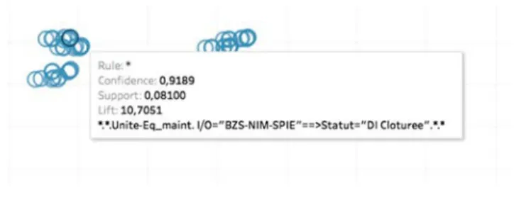
Fig. 10. Superimposition of rules.

The comparison between the breakdown duration and the criticality of the equipment is also of interest, showing that very few critical machines need more than 3 h to be repaired but that the number of machines of “high” criticality having been repaired in 2 h is the same than for machines of “medium” criticality.

It can also be noticed that one rule links the cause description “operator error” and the criticality of an equipment. This rule concerns an equipment of “high” criticality, denoting that errors occur more often on highly critical machines. This paradoxical result suggests to improve the training of the operators on highly critical equipment, often more complex than the others.

Maint:

Objective analysis: A lot of rules with support = 0.6662 can be

distinguished on the graph of Fig. 8. When using the spreadsheet to

select them, it can be seen that 30 rules link no production shutdown, curative maintenance, under contract and status = closed. This means that many curative maintenance operations have been conducted

without stopping production, which may set into question the interest

maintenance services at a customer’s site).

The second shows that only 10% of contractual breakdowns result in a shutdown. The selection of a “vital” level of criticity as antecedent of the rules allows to obtain 957 rules describing failures on vital equipment. The consequent parts of these rules allow to check that none of these failures resulted in stopping the machine, and none was non- contractual, which is a very good result that can be used by Maint to demonstrate its effectiveness to its customer.

24% of the failures on vital equipment concern the same domain (electrical, electromechanical, electronic). Improving the availability on vital equipment clearly requires an investigation on this sector.

The rules with confidence = 1 (11032) mainly link the references of pieces of equipment, their description, a high criticality and an absence of production shutdowns. When the rules with confidence = 1 expres- sing an equipment downtime are selected, 51 rules are found, con- cerning two devices: one allowing to store and distribute sand, and a mobile gateway. In the second case, it can be seen that the downtime of this strategic equipment has not required to stop production. The four corresponding rules, summarizing 369 transactions, nevertheless ex- hibit a recurrent problem that should be addressed.

Sem:

This rule base is interesting since its class diagram shows that it contains unusual details on the operator in charge of the maintenance activity. Moreover, the relatively limited number of rules allow a better legibility of the graphical representation.

Objective analysis: Rules with low support have widely dispersed confidence. On the contrary, few rules have high support and con- fidence. Especially, two symmetrical rules have again a maximum of preventive maintenance on some specific machines.

The two rules on the top right corner of Fig. 8 state that the waiting

cause is empty for most contractual failures. Then, many rules include

the “closed” status, shared by most transactions. _{The graph of Fig. 9 is more interesting, since it allows to distinguish}

support and confidence (top-right corner of Fig. 8):

Maint_type:”Curative”= > Family_name=”DGF” conf = 1 lift = 1 Family_name=”DGF”= > Maint_type:”Curative” conf = 0.96 lift = 1 sup = 0.96 sup = 0.96

three groups of rules on the top of the graph. Nevertheless, these groups are difficult to explore using the graphs since, even when zooming, many rules are superimposed and cannot be visualized (see the “*” in

Fig. 10 denoting multiple different attributes or values). This shows the limits of the visualization of such a number of rules on the same gra- phic.

Subjective analysis: The Maint class model is one of the most comprehensive, offering many opportunities to define a path of interest

between the attributes of the objects. On the base of the model of Fig. 5,

it can for instance be interesting to try to link: – waiting causes to causes of failures or failures, – production shutdown to equipment or failures, – equipment to failure domains, etc.

There are 15 different waiting causes in the data base, but none of them reaches the 8% support threshold that would allow to create a rule.

Indeed, Waiting_cause=”empty” is the only value present in the rules (representing 12,310 transactions on 13000). This shows the in- terest to be able to still decrease the minsup, and to manage more rules. Failures have resulted in production stoppages in 1240 transactions. 15 rules thus include a production stoppage, among which the most interesting ones are the two symmetrical rules:

Production_stop=”+”= > Non-contractual=”-“ sup = 0.1 conf = 1 lift = 1

These rules mean that nearly all the transactions (sup = 0.96) concern curative activities on the system DGF, also concerned by some rare preventive maintenance activities (637 transactions on 14524).

Many rules of confidence 1 are accessible (top line of the graph of

Fig. 8) linking for instance the category of the actor and the family of the system, or the family and the type of action. A good example is:

Maint_type=”Curative”.

Actor_category=”Planner”= > Family_name=”DGF” sup = 0.20 conf = 1 lift = 1

showing that planners doing curative actions always intervene on the system family “DGF”.

Many rules with high confidence and lift are grouped in the points

at the top of Fig. 9: coming back to the spreadsheet, it can be seen that

996 rules have a confidence = 1 and a lift = 1. They express strong but poorly informative relationships in the database, linked to empty fields: in a transaction, when a field is empty, many others are usually also empty.

Subjective analysis: The class diagram suggests interesting possible correlations, for instance between actor category and maintenance event type, duration and cause, duration and symptom, etc.

When selecting the filters, three categories of actors appear: planner (3104 transactions), technician (9177 transactions) and equipment owner (2238 transactions).

Table 3

Comparison of the results.

Data model Trans /rules Genericity Pos correlations

Non-contractual=”-“= > Production_stop=”+” sup = 0.1 conf =

0.1 lift = 1

The first indicates that no production stoppage is a “non-con- tractual” breakdown, which is a good indicator for the company for which Maint works: indeed, the critical resources are covered by the maintenance contract (let us remind that the company provides

Aero Basic 0,002 Varied Low

Auto Ambiguous 0,352 Poor High

Pharm Standard 0,005 Poor High

Maint Complex 0,020 Varied Low

Sem Standard 0,218 Poor Average

Ru.e: • Conf1cence· 0,9189

Suppo,t 0,08100

[;ft 10,7051