Wavelets on the Interval and Fast Wavelet Transforms

Partager "Wavelets on the Interval and Fast Wavelet Transforms"

N/A

Protected

Année scolaire: 2021

Info

Télécharger

Protected

Academic year: 2021

Partager "Wavelets on the Interval and Fast Wavelet Transforms"

Copied!

Chargement.... (Voir le texte intégral maintenant)

Télécharger maintenant ( 28 Page )

Texte intégral

Figure

$FIG. 2. Low pass filtering scheme for the "folded" case, going from V!o\d to V'~1d, in the case where support cf> = [ -2, 2], i.e., only h_ 2 , h_" h 0 ,$

FIG. 3. Schematic representation of the non-zero H'!_,"" (solid lines), h~~:: (dashed lines) for k = -2, -1, 0, 1 in the case N = 3

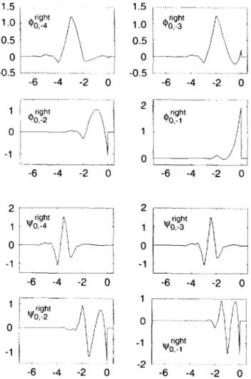
FIG. 4. The orthonormal scaling functions and wavelets for N = 2 in Meyer's construction, at a left edge (i.e., on [ 0, oo)) or a right edge (on ( -oo, 0])

FIG. Sa. The orthonormal scaling functions and wavelets for N = 4 in Meyer's construction on the half line [ 0, oo)

Références

Télécharger maintenant ( PDF - 28 Page - 0.92 MB )

Documents relatifs