Article
Detecting Local Drivers of Fire Cycle Heterogeneity
in Boreal Forests: A Scale Issue
Annie Claude Bélisle1,*, Alain Leduc2, Sylvie Gauthier3, Mélanie Desrochers4, Nicolas Mansuy3, Hubert Morin5and Yves Bergeron6
1 Institut de Recherche sur les Forêts, Université du Québec en Abitibi-Témiscamingue and Centre d’étude de la forêt, Case Postale 8888, Succursale Centre-Ville Montréal, Quebec, QC H3C 3P8, Canada
2 Département des Sciences Biologiques, Chaire Industrielle CRSNG UQAT-UQAM en Aménagement Forestier Durable, Université du Québec à Montréal and Centre d’étude de la forêt, Case Postale 8888, succursale Centre-Ville Montréal, Quebec, QC H3C 3P8, Canada; [email protected]
3 Natural Resources Canada, Canadian Forest Service, Laurentian Forestry Centre, 1055 du PEPS, PO Box 10380, Stn. Sainte-Foy, Québec, QC G1V 4C7, Canada; [email protected] (S.G.); [email protected] (N.M.)
4 Centre d’étude de la forêt, Case Postale 8888, Succursale Centre-Ville Montréal, Montreal, QC H3C 3P8, Canada; [email protected]
5 Département des Sciences Fondamentales, Université du Québec à Chicoutimi, 555 Boulevard de l’Université, Chicoutimi, QC G7H 2B1, Canada; [email protected]
6 Chaire Industrielle CRSNG UQAT-UQAM en Aménagement Forestier Durable, Université du Québec en Abitibi-Témiscamingue and Université du Québec à Montréal, 445, boul. de l’Université, Rouyn-Noranda, QC J9X 5E4, Canada; [email protected]
* Correspondence: [email protected]; Tel.: +1-877-870-8728 (ext. 4353) Academic Editors: Timothy A. Martin and Eric J. Jokela
Received: 30 May 2016; Accepted: 29 June 2016; Published: 12 July 2016
Abstract:Severe crown fires are determining disturbances for the composition and structure of boreal forests in North America. Fire cycle (FC) associations with continental climate gradients are well known, but smaller scale controls remain poorly documented. Using a time since fire map (time scale of 300 years), the study aims to assess the relative contributions of local and regional controls on FC and to describe the relationship between FC heterogeneity and vegetation patterns. The study area, located in boreal eastern North America, was partitioned into watersheds according to five scales going from local (3 km2) to landscape (2800 km2) scales. Using survival analysis, we observed that dry surficial deposits and hydrography density better predict FC when measured at the local scale, while terrain complexity and slope position perform better when measured at the middle and landscape scales. The most parsimonious model was selected according to the Akaike information criterion to predict FC throughout the study area. We detected two FC zones, one short (159 years) and one long (303 years), with specific age structures and tree compositions. We argue that the local heterogeneity of the fire regime contributes to ecosystem diversity and must be considered in ecosystem management.
Keywords:forest ecology; fire cycle; multi-scale models; survival analysis; physiographic drivers
1. Introduction
Patterns and processes of boreal forests are highly determined by large-scale disturbance regimes [1,2]. In North America, stand-replacing crown fires [3–5] shape landscapes in patchworks where forest stands differ in their age, internal structure and composition [6,7]. Disturbance regime parameters are used as benchmarks by forest managers concerned with ecosystem management and the natural range of variability [8,9]. Understanding fire regime drivers and their consequences on forest landscapes is hence a key issue for boreal landscape ecology, resilience and management [10–13].
Forests 2016, 7, 139 2 of 21
Fire frequency, or rate, is a parameter of fire regime expressing the mean proportion of area that is burned yearly in the region of interest [14]. It can also be expressed by the concept of fire cycle (FC), having both area- and point-based meanings and interpretations [15]. From the area-based perspective, it is defined as the time required (year) to burn an area equivalent to the region of interest and is mathematically the inverse of annual burn rate [15]. It thus assumes homogeneity over the entire region of interest. From the point-based perspective, FC is the mean time interval (year) between fires during a certain period of time (e.g., the Holocene) for a single location. FC in a region drives landscape age-structure [16], species composition [17] and succession pathways [18–20]. Easily transferable to forest ecosystem management, FC and associated landscape age-structure are useful to compare harvested and natural landscapes [10,21]. For example, FC was used to describe old-growth forests’ natural range of abundance and to highlight their depletion in managed landscapes of eastern Canada [22]. In this research, we stress the homogeneity assumption and propose a way to deal with a heterogeneous area.
FC spatial variability depends on the interactions between top-down controls, such as weather (regional to global scales), and bottom-up controls, such as fuel availability, quality and connectivity (local to landscape scale) [23–25]. In boreal North America, large fires, even if infrequent compared to small fires, are responsible for most of the burned area (3% of the fires account for 97% of burned area in Canada) [3]. Their occurrence and distribution are generally assumed to be driven by weather conditions [26,27]. FC hence follows a continental climate gradient, going from the dry inland continent where fires are recurrent to the wet East Coast where fires are rare [28]. Additional spatial variability in FC is observed at the regional scale and may be explained by soil drainage and regional fire weather [28,29]. It is a more complicated task to identify local drivers of FC because of large and severe fires, making it impossible to compare for instance the number of fires or the area burned in localities. Researchers interested in bottom-up drivers of FC need to turn towards historical fire data collected with dendrochronology or soil and lake charcoal deposits [30–33]. Local variability may also be captured with simulations based on fire behavior models [24,34]. The first presents the advantage of describing an empirical reality, but requires greater effort for historical data acquisition. The second allows covering greater spatial extents and taking into account the mechanisms involved, but relies mostly on simulations.
In eastern North America, FC is generally assumed to be regionally homogeneous. It ranges from ~100 years–>500 years for the last 300 years and from 388–645 for the recent period (1940–2003) [29,35,36]. However, vegetation patterns are sometimes in apparent contradiction with the estimated FC within the homogeneous FC assumption. For instance, FC reported for jack pine (Pinus banksiana Lamb.) stands is often shorter than regional FC, partly because of low-severity fire occurrence (e.g., [33,37]. Moreover, jack pine should theoretically be excluded from zones where fire frequency is low because of its serotinous cones, which need extreme heat to open [18,32,38]. Otherwise, its distribution extends on sandy soils of regions where historical FC exceeds species longevity [36,39]. Driving factors of FC recently appeared to be highly scale dependent, making studies undertaken on a single scale unable to capture FC spatial complexity [40–43]. A multi-scale approach is necessary to investigate the influence of both local and regional factors on FC. Measuring and understanding this relation is important for fire ecology, modeling and forest management.
The objective of this research is to assess the relative contributions of local versus regional controls on FC and to describe the relation between FC and vegetation succession patterns in boreal forests of Eastern Canada. We hypothesize that: (1) FC is primarily influenced by bottom-up processes driven by coarse topographic features, especially valleys where dry soils in conjunction with wind corridors may enhance fire frequency [44,45] and hills that may act as fire breaks [46]; (2) FC is locally shorter where soils are well drained [29,47] and longer where fire breaks are abundant [48]; and (3) the vegetation succession pathway spatial distribution goes along with the FC spatial distribution.
In this paper, we assess the relationship between FC and physiographic variables for a boreal region of eastern Canada. We used survival analysis to model FC with time since fire data covering
Forests 2016, 7, 139 3 of 21
the last 300 years. We addressed the scale issue by partitioning the study area into five scale classes, from local to landscape, based on watershed Strahler order. All physiographic variables were thus measured for five scales in order to identify the most accurate to predict FC. Model selection based on the Akaike information criterion was performed to choose the “best” variable scale combinations. 2. Materials and Methods
2.1. Study Area
The study area (Figure1) covers 540,300 ha in the continuous boreal forest of eastern North America (71˝151 W–72˝451 W, 49˝361 N–50˝591 N). Black spruce (Picea mariana Mill.) feather moss forest is the most abundant ecological type [49]. Jack pine, paper birch (Betula papyrifera Marsh.) and trembling aspen (Populus tremuloides Michx.) are present in some young forests. Balsam fir (Abies balsamea Mill.) is co-dominant with black spruce in some old-growth forests [39]. Elevation ranges between 120 m and 870 m, striking a contrast between the typical rounded hills of the Boreal Shield and the valleys of the deeply embedded rivers [50,51]. Hydrography is structured by two north-south-oriented rivers (Mistassibi and Mistassibi Nord-Est). Surficial materials are mainly composed of glacial tills with rocky outcrops and fluvioglacial sands following river beds. Some depletion moraines are located on the northern part of the study area; organic surficial materials are also common [51,52]. Mean temperature ranges between a minimum of 6˝C–19˝C and a maximum of 21˝C–25˝C in July and between a minimum of ´29˝C–´25˝C and a maximum of ´14˝C–´10˝C in January (1971–2001). Average annual precipitation ranges between 900 mm and 1200 mm, 30%–35% of which falls as snow [50,53].
Forests 2016, 7, 139 3 of 22 In this paper, we assess the relationship between FC and physiographic variables for a boreal region of eastern Canada. We used survival analysis to model FC with time since fire data covering the last 300 years. We addressed the scale issue by partitioning the study area into five scale classes, from local to landscape, based on watershed Strahler order. All physiographic variables were thus measured for five scales in order to identify the most accurate to predict FC. Model selection based on the Akaike information criterion was performed to choose the “best” variable scale combinations. 2. Materials and Methods 2.1. Study Area
The study area (Figure 1) covers 540,300 ha in the continuous boreal forest of eastern North America (71°15′ W–72°45′ W, 49°36′ N–50°59′ N). Black spruce (Picea mariana Mill.) feather moss forest is the most abundant ecological type [49]. Jack pine, paper birch (Betula papyrifera Marsh.) and trembling aspen (Populus tremuloides Michx.) are present in some young forests. Balsam fir (Abies balsamea Mill.) is co‐dominant with black spruce in some old‐growth forests [39]. Elevation ranges between 120 m and 870 m, striking a contrast between the typical rounded hills of the Boreal Shield and the valleys of the deeply embedded rivers [50,51]. Hydrography is structured by two north‐south‐oriented rivers (Mistassibi and Mistassibi Nord‐Est). Surficial materials are mainly composed of glacial tills with rocky outcrops and fluvioglacial sands following river beds. Some depletion moraines are located on the northern part of the study area; organic surficial materials are also common [51,52]. Mean temperature ranges between a minimum of 6 °C–19 °C and a maximum of 21 °C–25 °C in July and between a minimum of −29 °C–−25 °C and a maximum of −14 °C–−10 °C in January (1971–2001). Average annual precipitation ranges between 900 mm and 1200 mm, 30%–35% of which falls as snow [50,53].
Figure 1. Stand origin map [21] within the study area, including fire delineation (1900–2010) from aerial photos and time elapsed since last fire (TSF) sampling points.
Figure 1. Stand origin map [21] within the study area, including fire delineation (1900–2010) from aerial photos and time elapsed since last fire (TSF) sampling points.
Forests 2016, 7, 139 4 of 21
As elsewhere in the boreal forest of eastern North America, the landscape is subject to severe crown fires [4]. FC in the region is estimated at 247 years for the last 300 years and at 375 years for the recent period (1949–2009). The mean fire size was 10,000 ha between 1970 and 2010 [13]. Most of the burned area is attributable to four fire decades: the 1820s, 1860s, 1920s and 2000s [13]. The study area is located in a homogeneous fire region according to [28]. No influence of latitude and longitude on FC has been observed [39].
Located on public tenures, the study area has been partly, but extensively managed for wood supply since the 1970s [54,55]. Before 1950, the landscape remained almost free from human activities, with a native population density estimated at 0.005 individuals/km2[56]. The closest villages are located 70 km south and were settled between 1870 and 1930 [57].
2.2. Environment Delineation and Scaling
We designed environment delineation and scaling according to the drainage network and associated watersheds. Watersheds rely on water bodies with a hierarchical drainage network, making them embedded and scalable. Strahler order [58] is used to classify rivers and their catchment areas according to their importance (see AppendixAFigureA1). Moreover, contrary to administrative borders or the circular buffers generally used (e.g., [30,40]), they rely on real physiographic features [59].
Watersheds were delineated using the ArcGIS 10.1 (Esri, Redlands, CA, USA) Hydrology toolbox (see TableA1). Strahler orders were computed using a 20-m flow accumulation raster in which a cell was considered a river when its flow accumulation was greater than 16 ha (400 cells, as suggested by the ArcGIS 10.1 help module). Order 1 rivers were fuzzy and did not fit well with previously mapped rivers, so we only considered Orders 2–6, reported as 1–5. We delineated watersheds for every river (manual pour-point distribution, Watershed tool), defined by their hierarchical importance. We consider Orders 1 and 2 as local scale, Order 3 as middle scale and Orders 4 and 5 as landscape scale. The number of watersheds exponentially decreases when the scale gets coarser, ranging from 3736 watersheds of Order 1 to 6 of Order 5 (Figure2). Conversely, mean watershed size increases exponentially with order, ranging from 2.9 km2(Order 1) to 1782.5 km2(Order 5). Watersheds generally present an elongated shape and follow a north-south axis, especially at the middle and landscape scales.
Forests 2016, 7, 139 5 of 22
Figure 2. Watershed delineation for Strahler Orders 1–5, grouped into local (Orders 1 and 2), middle (Order 3) and landscape (Orders 4 and 5) scales. n = number of watersheds, = mean area (km2). In order to test the effect of physiographic factors on FC, we built scale‐dependent metrics of soil drying potential, fire break density, terrain complexity and slope position (Table 1). This means that for a single location in the study area, those metrics take on different values depending on the scale at which they are measured. Spatial analyses were processed on ArcGIS 10.0 using a 20‐m raster from which water bodies were excluded (except for fire break density calculation).
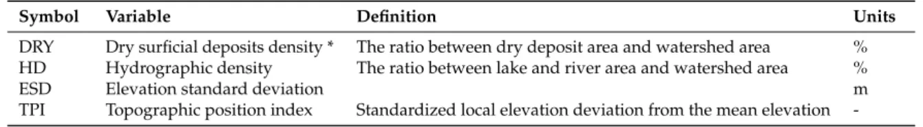
Table 1. Definition of explanatory (predictor) variables (p in the Cox proportional hazard model, see Equation (1)).
Symbol Variable Definition Units
DRY Dry surficial deposits density * The ratio between dry deposit area and watershed area %
HD Hydrographic density The ratio between lake and river area and watershed area %
ESD Elevation standard deviation m
TPI Topographic position index Standardized local elevation deviation from the mean elevation ‐
* Dry materials of the study area were mainly composed of sandy textured fluvioglacial and juxtaglacial deposits, disintegration moraines and rocky outcrops.
ln h t ln h t β X ⋯ β X 1 (1)
h(t), Hazard to survive (not to burn) to time t; h t , Unspecified baseline hazard; P, Number of predictor variables; β, Coefficient estimate; X, Predictor value.
We hypothesized that well‐drained soils enhance combustible dryness and inflammability and thus shorten FC. We used a surficial materials classification [29] to make the distinction between high and low soil drying potential. Dry materials of the study area were mainly composed of sandy textured fluvioglacial and juxtaglacial deposits, disintegration moraines and rocky outcrops. Dry surficial material density (DRY) is thereby defined as the proportion of an area occupied by dry deposits on a given area. Hydrology density (HD) is defined as the proportion of an area occupied by water bodies (lakes and rivers) and is used as an indicator of fire break abundance [48]. HD was computed using a water body map (1:50,000) provided by the Government of Canada [50]. Literally defined as the elevation standard deviation, Elevation standard deviation (ESD) is an index of topography ruggedness and may also be associated with fire break density. The more the terrain presents slopes and hills, the higher the ESD. Finally, the topographic position index (TPI) is a measure of slope position [63] and is defined as the difference between local elevation and mean
Figure 2.Watershed delineation for Strahler Orders 1–5, grouped into local (Orders 1 and 2), middle (Order 3) and landscape (Orders 4 and 5) scales. n = number of watersheds, x = mean area (km2).
Forests 2016, 7, 139 5 of 21
2.3. Data Collection
The method used to study the spatial distribution of FC uses historical time since fire data. When assessing FC, spatial extent can be traded for temporal depth and vice versa. For example, to assess FC for a precise location (point-based), paleoclimatic data are needed. Alternatively, to assess FC for a whole region (area-based), annual burn rate (area burned/year) by itself allows calculating FC. This research is at the mid-point between both perspectives. Using historical data allowed us to divide the study area into smaller zones according to their specific FC.
We used a stand-origin map to derive FC from the time elapsed since last fire (TSF) distribution [60]. This methodology has proven to be useful for regimes of severe and infrequent fires where fire scars are rare and long time series are needed [31,32,36,61]. TSF point data (n = 144, density = 1 point every 36 km2) are derived from government fire registers (Direction de la protection des forêts, 1950–2010), vegetation databases [62], aerial photographs (1948) and tree ring analysis (see [21] for details on data collection) (Figure1). TSF data are scattered on a grid (resolution: 6 km) with one random point in every cell. TSF is considered real when traces of the last fire make it possible to determine a fire year (˘ 10 years) (from aerial photos or even-aged tree distribution); otherwise, a minimum and censored TSF, corresponding to the age of the oldest tree sampled, is attributed [62].
In order to test the effect of physiographic factors on FC, we built scale-dependent metrics of soil drying potential, fire break density, terrain complexity and slope position (Table1). This means that for a single location in the study area, those metrics take on different values depending on the scale at which they are measured. Spatial analyses were processed on ArcGIS 10.0 using a 20-m raster from which water bodies were excluded (except for fire break density calculation).
lnh ptq “ lnh0ptq ` β1X1`. . . ` βpXp p1q (1) h(t), Hazard to survive (not to burn) to time t; h0ptq, Unspecified baseline hazard; P, Number of predictor variables; β, Coefficient estimate; X, Predictor value.
Table 1.Definition of explanatory (predictor) variables (p in the Cox proportional hazard model, see Equation (1)).
Symbol Variable Definition Units
DRY Dry surficial deposits density * The ratio between dry deposit area and watershed area %
HD Hydrographic density The ratio between lake and river area and watershed area %
ESD Elevation standard deviation m
TPI Topographic position index Standardized local elevation deviation from the mean elevation
-* Dry materials of the study area were mainly composed of sandy textured fluvioglacial and juxtaglacial deposits, disintegration moraines and rocky outcrops.
We hypothesized that well-drained soils enhance combustible dryness and inflammability and thus shorten FC. We used a surficial materials classification [29] to make the distinction between high and low soil drying potential. Dry materials of the study area were mainly composed of sandy textured fluvioglacial and juxtaglacial deposits, disintegration moraines and rocky outcrops. Dry surficial material density (DRY) is thereby defined as the proportion of an area occupied by dry deposits on a given area. Hydrology density (HD) is defined as the proportion of an area occupied by water bodies (lakes and rivers) and is used as an indicator of fire break abundance [48]. HD was computed using a water body map (1:50,000) provided by the Government of Canada [50]. Literally defined as the elevation standard deviation, Elevation standard deviation (ESD) is an index of topography ruggedness and may also be associated with fire break density. The more the terrain presents slopes and hills, the higher the ESD. Finally, the topographic position index (TPI) is a measure of slope position [63] and is defined as the difference between local elevation and mean environment elevation, divided by environment ESD. High slope position locations may be less prone to fire because of a colder and wetter climate creating a persistent snow cover during spring [46]. A TPI below ´1 indicates valleys
Forests 2016, 7, 139 6 of 21
and down-slopes; a TPI between ´1 and 1 indicates mid-slopes; and a TPI greater than 1 indicates up-slopes and mountain tops.
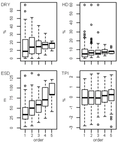
The variable distribution changes with scale, so for a single point in space, the same variable can take on different values according to the scale. DRY, HD, ESD and TPI distributions throughout the study area are presented for all five scales (Figure3). The range of DRY and HD narrows when the scale gets coarser, so their distribution follows small patches in the study area. ESD range increases with scale, so the topography is characterized by coarse features. TPI range remains the same as expected because this metric is normalized. For TPI, HD and ESD, watershed is described by a unique value, so for Order 5 watersheds, they can take on only six possible values.
Forests 2016, 7, 139 6 of 22
environment elevation, divided by environment ESD. High slope position locations may be less prone to fire because of a colder and wetter climate creating a persistent snow cover during spring [46]. A TPI below −1 indicates valleys and down‐slopes; a TPI between −1 and 1 indicates mid‐slopes; and a TPI greater than 1 indicates up‐slopes and mountain tops. The variable distribution changes with scale, so for a single point in space, the same variable can take on different values according to the scale. DRY, HD, ESD and TPI distributions throughout the study area are presented for all five scales (Figure 3). The range of DRY and HD narrows when the scale gets coarser, so their distribution follows small patches in the study area. ESD range increases with scale, so the topography is characterized by coarse features. TPI range remains the same as expected because this metric is normalized. For TPI, HD and ESD, watershed is described by a unique value, so for Order 5 watersheds, they can take on only six possible values.
Figure 3. Dry surface deposits density (DRY) (%), Hydrographic density (HD) (%), Elevation Standard Deviation (ESD) (m) and Topographic position index (TPI) (%) distributions (see Table 1) for Orders 1–5 (see Figure 2). Horizontal lines represent the 25th, 50th and 75th percentiles, and whiskers indicate the range. Dots represent values for which the distance from the box is 1.5‐times greater than the length of the box. 2.4. Survival Analysis Survival analysis tests the relation between two or more variables and includes censored data that are only partially known [64]. TSF is censored when the year of the last fire is unknown so the only information we have is a minimum time elapsed without fire. We used the Cox proportional hazard model (Equation (1)), a semi‐parametric survival analysis, to model the influence of physical environment on fire frequency [30,31,64]. Statistical analyses were computed in the software R (version 2.15.1, The R Foundation for Statistical Computing, Vienna, Austria), package survival [65]. We first tested the effect of environmental variables and scales on fire hazard using and comparing single‐variable survival analysis (see Table 2 for the FC modeling main steps). We tested
Figure 3.Dry surface deposits density (DRY) (%), Hydrographic density (HD) (%), Elevation Standard Deviation (ESD) (m) and Topographic position index (TPI) (%) distributions (see Table1) for Orders 1–5 (see Figure2). Horizontal lines represent the 25th, 50th and 75th percentiles, and whiskers indicate the range. Dots represent values for which the distance from the box is 1.5-times greater than the length of the box.
2.4. Survival Analysis
Survival analysis tests the relation between two or more variables and includes censored data that are only partially known [64]. TSF is censored when the year of the last fire is unknown so the only information we have is a minimum time elapsed without fire. We used the Cox proportional hazard model (Equation (1)), a semi-parametric survival analysis, to model the influence of physical environment on fire frequency [30,31,64]. Statistical analyses were computed in the software R (version 2.15.1, The R Foundation for Statistical Computing, Vienna, Austria), package survival [65].
We first tested the effect of environmental variables and scales on fire hazard using and comparing single-variable survival analysis (see Table2for the FC modeling main steps). We tested 20 proportional hazard models (function coxph) (4 variables ˆ 5 scales) [66]. DRY was log-transformed to meet the
Forests 2016, 7, 139 7 of 21
proportional hazard model assumption, i.e., the relative risk for each stratum must remain the same over time. Models were performed with a single dataset of 144 TSF points.
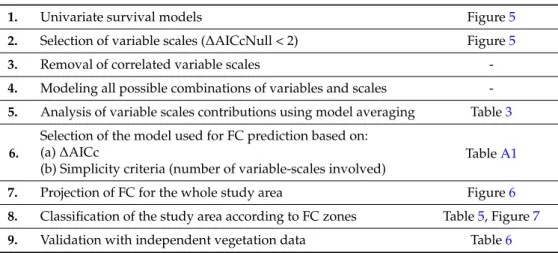
Table 2.Main steps for the model selection and projection.
1. Univariate survival models Figure5
2. Selection of variable scales (∆AICcNull < 2) Figure5
3. Removal of correlated variable scales
-4. Modeling all possible combinations of variables and scales
-5. Analysis of variable scales contributions using model averaging Table3
6.
Selection of the model used for FC prediction based on:
TableA1
(a)∆AICc
(b) Simplicity criteria (number of variable-scales involved)
7. Projection of FC for the whole study area Figure6
8. Classification of the study area according to FC zones Table5, Figure7
9. Validation with independent vegetation data Table6
Model accuracy and performance were compared on the basis of their second-order Akaike information criterion (AICc), informing on the balance between model complexity and predictivity [67]. Wald test and log-likelihood ratio test scores (p < 0.05) inform on the goodness of fit compared to the null model [64]. Linear predictors indicate the sense and the relative magnitude of the relation. Confidence intervals (95%) on linear predictors were computed with bootstrapping (1000 resamplings with replacement from the original dataset, n = 144). We also suspected an overwhelming effect of recent fires, so we sequentially excluded fire years (2009, 2007, 2005) to check their influence on results [68]. Only relevant variable-scale combinations, with an AICc difference with null model (∆AICcNull) > 2 [69], were considered for multi-scale models. If two variable scales were correlated (Pearson’s coefficient >0.7), one of them was removed in further analysis. After selecting significant and uncorrelated variables and scales, we then tested existing combinations of variables and scales (CRAN R package MuMin) [70]). The potential best models were identified by an AICc difference with the lowest AICc (∆AICc) <2, indicating a balance between model complexity and predictivity [67,69]. Variables relative contributions, or cumulated weights, were calculated by model averaging (Σ (linear predictor ˆ model weight)) [67].
2.5. FC Prediction and Distribution
In accordance with the parsimony principle, we selected the simplest model (i.e., involving the lower number of variables and scales) among the set of potential best models. For instance, Fictive Model 1 (DRY1 + HD1) would be chosen over Model 2 (DRY1 + HD3) or Model 3(DRY1 + HD1 + ESD1). Mean annual hazard was estimated for the 200 first years (1810–2010) of the baseline hazard function (basehaz in package survival [66]) and multiplied by the hazard ratio:
hiptq hmptq
“ e Xiβ
eXmβ (2)
( hmptq = mean hazard at time t, Xm= mean predictor) to predict annual burn rate, which is the inverse of FC. We predicted FC with the previous equation both for the original dataset and for the whole study area raster. For interpretation and validation purposes, FC was grouped into classes in accordance with the shape and the extent of FC distribution. The number of classes was dictated by the number of modes and their limits by the breakpoints between modes. FC was calculated for each class of the TSF dataset using their specific basehaz functions. We calculated a 95% confidence interval on FC by bootstrapping (1000 resamplings with replacement from the original dataset, n = 144).
Forests 2016, 7, 139 8 of 21
Landscape age structure directly depends on FC [16]. We validated the model by testing if observed vegetation age-structures in the study area were consistent with the predicted FC. We used the photo-interpreted vegetation database (SIFORT) [52], which provides information on stands’ time since disturbance and composition with a resolution of 14 ha [71]. Although inventories exist for the decades of 1980, 1990, 2000 and 2010, we restricted analysis to the 1980s data to minimize the influence of forest management. Early succession forests (TSF < ~100 years) were recognized by delineated fires or by the presence (or dominance) of post-fire species (jack pine, paper birch (Betula papyrifera Marsh.), trembling aspen) [17,39]. Late succession forests were recognized by the presence of old-growth species, such as balsam, and by traces of insect outbreaks affecting specifically this species [72]. Pure black spruce stands, which can grow in all succession stages, were considered early-succession when the photo-interpreted age was below 90 years; otherwise, their status remained unknown. We expect a higher abundance of young forests where FC is short and a higher abundance of old-growth forests where FC is long. Succession stage abundances were compared between short and long FC with contingency table analysis (chi-square and Freeman–Tukey deviate).
2.6. Vegetation Composition
We hypothesized that forest composition is influenced by FC, especially in young forests. We identified post-fire cohorts throughout the study area according to the fire map described previously (1900–2010). We classified young forests into composition groups, corresponding to different succession pathways: jack pine (presence), broadleaf (presence) and black spruce (pure) [39]. Young forest succession pathway distributions were compared between short and long FC with contingency table analysis using chi-square and Freeman–Tukey deviate. Jack pine should theoretically be restricted to young forests in areas where FC is <200 years [18].
3. Results
3.1. Time since Fire Distribution
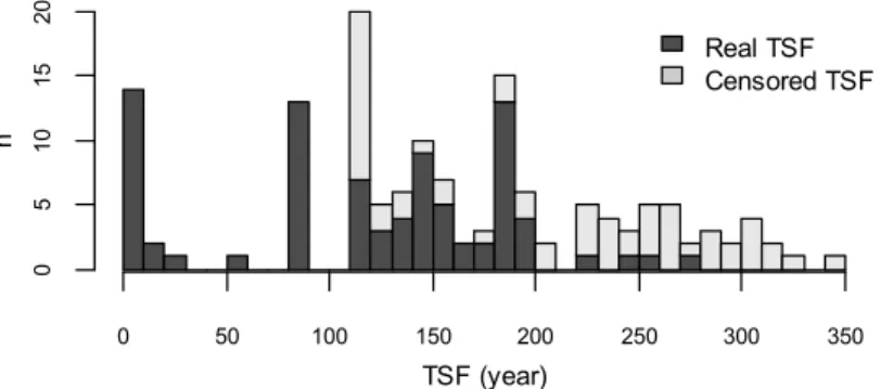
TSF is estimated for 144 locations throughout the study area. We were able to date the last fire (˘10 years) for 60% of these locations, while a minimum TSF, generally based on the age of the oldest tree, was determined for the remaining 40% (Figure4). TSF (including both real and minimum age) ranges from 0–340 years.
Forests 2016, 7, 139 8 of 22
decades of 1980, 1990, 2000 and 2010, we restricted analysis to the 1980s data to minimize the influence of forest management. Early succession forests (TSF < ~100 years) were recognized by delineated fires or by the presence (or dominance) of post‐fire species (jack pine, paper birch (Betula papyrifera Marsh.), trembling aspen) [17,39]. Late succession forests were recognized by the presence of old‐growth species, such as balsam, and by traces of insect outbreaks affecting specifically this species [72]. Pure black spruce stands, which can grow in all succession stages, were considered early‐succession when the photo‐interpreted age was below 90 years; otherwise, their status remained unknown. We expect a higher abundance of young forests where FC is short and a higher abundance of old‐growth forests where FC is long. Succession stage abundances were compared between short and long FC with contingency table analysis (chi‐square and Freeman–Tukey deviate). 2.6. Vegetation Composition
We hypothesized that forest composition is influenced by FC, especially in young forests. We identified post‐fire cohorts throughout the study area according to the fire map described previously (1900–2010). We classified young forests into composition groups, corresponding to different succession pathways: jack pine (presence), broadleaf (presence) and black spruce (pure) [39]. Young forest succession pathway distributions were compared between short and long FC with contingency table analysis using chi‐square and Freeman–Tukey deviate. Jack pine should theoretically be restricted to young forests in areas where FC is <200 years [18]. 3. Results 3.1. Time since Fire Distribution TSF is estimated for 144 locations throughout the study area. We were able to date the last fire (± 10 years) for 60% of these locations, while a minimum TSF, generally based on the age of the oldest tree, was determined for the remaining 40% (Figure 4). TSF (including both real and minimum age) ranges from 0–340 years.
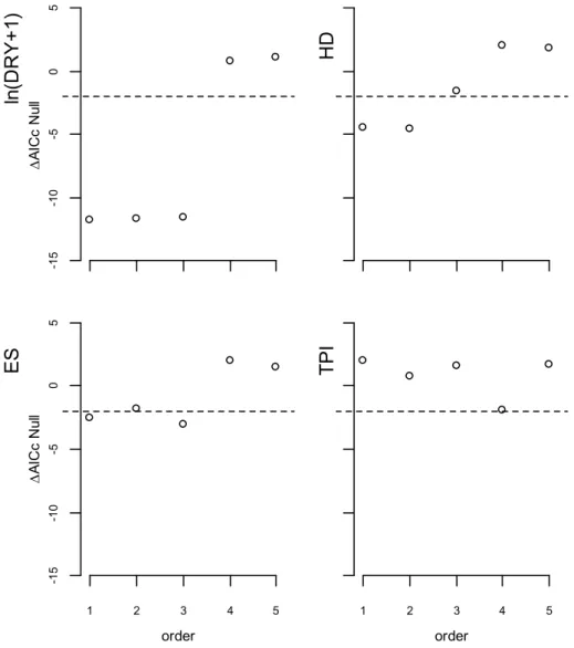
Figure 4. Real and censored (minimum) TSF distributions, grouped in 10‐year age classes (n = number of TSF data). 3.2. FC Modeling Single variable models are compared to the difference of AICc with the null model (∆AICcNull) (Figure 5). ln(DRY + 1) at local and middle scales has the best predictive power (∆AICcNull between −11.5 and −11.8). HD performs better at the local scale with ∆AICcNull of −4.5. For ESD at local and middle scales, ∆AICc ranges between −2.5 and −3.0. Finally, TPI has not shown any explicative power except at the landscape scale (Order 4), where ∆AICc is −1.9. Coefficients, confidence intervals, significance tests and controls for bias associated with recent fires are available in the Supplementary Material (Figure A2). TSF (year) n 0 5 10 15 20 0 50 100 150 200 250 300 350 Real TSF Censored TSF
Figure 4.Real and censored (minimum) TSF distributions, grouped in 10-year age classes (n = number of TSF data).
3.2. FC Modeling
Single variable models are compared to the difference of AICc with the null model (∆AICcNull) (Figure5). ln(DRY + 1) at local and middle scales has the best predictive power (∆AICcNull between ´11.5 and ´11.8). HD performs better at the local scale with∆AICcNull of ´4.5. For ESD at local and middle scales,∆AICc ranges between ´2.5 and ´3.0. Finally, TPI has not shown any explicative
Forests 2016, 7, 139 9 of 21
power except at the landscape scale (Order 4), where∆AICc is ´1.9. Coefficients, confidence intervals, significance tests and controls for bias associated with recent fires are available in the Supplementary Material (FigureA2).
Forests 2016, 7, 139 9 of 22
Significant variable‐scale associations according to ∆AICcNull are ln(DRY + 1)1, ln(DRY + 1)3,
HD1, ESD1 and ESD3. We also kept HD3 and TPI4 in the process, even if their performance was under
the ∆AICcNull to avoid missing significant interactions or patterns while knowing that they would be excluded from further analyses if no pattern emerged. Despite good individual performances, we excluded ln(DRY + 1)2, HD2 and ESR2 because they were too correlated with other variables. From
all possible combinations, fifteen had a ∆AICc < 2 and were thus considered as potential best models (Supplementary Material). Model averaging shows that the parameters that contribute the most are HD1, ln(DRY + 1)1 and ln(DRY + 1)3, which all had a cumulated weight greater than 65% (Table 3).
From the 15 potentially best models, we selected the simplest one to predict FC, in accordance with the parsimony principle. The selected model thus includes the proportion of dry surficial deposits and hydrologic density, both at the local scale, to predict FC (Table 4).
Figure 5. AICc difference with the null model (∆AICcNull) for the Cox univariate models with four variables (ln(DRY + 1), HD, ES, TPI) (see Table 1) and scale Orders 1–5 (see Figure 2). The dotted lines indicate ∆AICc = −2. Dots under the line are better than the null model [67,69], and full dots indicate variables qualified for model selection (Table 3). -1 5 -1 0 -5 0 5 AI C c N ul l
ln
(DRY
+
1)
HD
1 2 3 4 5 -1 5 -1 0 -5 0 5 order A ICc Nu llES
1 2 3 4 5 orderTP
I
Figure 5.AICc difference with the null model (∆AICcNull) for the Cox univariate models with four
variables (ln(DRY + 1), HD, ES, TPI) (see Table1) and scale Orders 1–5 (see Figure2). The dotted lines indicate∆AICc = ´2. Dots under the line are better than the null model [67,69], and full dots indicate variables qualified for model selection (Table3).
Significant variable-scale associations according to∆AICcNull are ln(DRY + 1)1, ln(DRY + 1)3, HD1, ESD1and ESD3. We also kept HD3 and TPI4 in the process, even if their performance was under the∆AICcNull to avoid missing significant interactions or patterns while knowing that they would be excluded from further analyses if no pattern emerged. Despite good individual performances, we excluded ln(DRY + 1)2, HD2 and ESR2 because they were too correlated with other variables. From all possible combinations, fifteen had a∆AICc < 2 and were thus considered as potential best models (Supplementary Material). Model averaging shows that the parameters that contribute the most are HD1, ln(DRY + 1)1and ln(DRY + 1)3, which all had a cumulated weight greater than 65% (Table3). From the 15 potentially best models, we selected the simplest one to predict FC, in accordance with the parsimony principle. The selected model thus includes the proportion of dry surficial deposits and hydrologic density, both at the local scale, to predict FC (Table4).
Forests 2016, 7, 139 10 of 21
Table 3.Relative importance of parameters (cumulated weight), coefficient averaged estimate and 95% confidence interval from multi-model inference for the DRY, HD, ESD and TRI selected orders.
Explanatory Variables Watershed Order Relative Importance (Cumulated Weight) Model-Averaged Estimate 95% Confidence Interval Lower Upper ln(DRY + 1) 1 0.73 0.1940 ´0.0073 0.5097 3 0.68 0.2789 ´0.0315 0.7927 HD 1 0.83 ´0.0337 ´0.0830 ´0.0020 3 0.32 ´0.0043 ´0.1039 0.0471 ESD 13 0.450.38 0.00260.0014 ´0.0029´0.0038 0.01430.0109 TRI 4 0.36 ´0.0426 ´0.3868 0.0543
Table 4. Coefficients and confidence intervals (CI), Wald test score (z) and p-values for the selected model.
Coefficients CI (2.5%) CI (97.5%) z Pr (>|z|)
ln(DRY + 1)1 0.355 0.170 0.546 3.798 0.000146
HD1 ´0.0430 ´0.0827 ´0.0154 ´2.510 0.012063
∆AICc 0.66
Likelihood ratio test = 21.94 on 2 df, p = 1.724-5. Wald test = 18.82 on 2 df, p = 8.177-5.
3.3. FC Distribution
For the original TSF dataset (n = 144), predicted FC ranges between 74 and 2041 years with a mean of 241 years (Figure6a). For the entire study area, it ranges from 60–8000 years with a mean of 224 years (Figure6b). The FC distribution has a bimodal shape for both the TSF dataset and the whole study area, so FC is classified into two groups, short and long. The break between modes is estimated to be located at 275 years according to the entire study area, so 73% belongs to the short FC zone while 27% belongs to the long FC zone. The difference between the FC of each zone is confirmed when FC and confidence intervals are estimated from the TSF distribution (Table5).
Forests 2016, 7, 139 10 of 22 Table 3. Relative importance of parameters (cumulated weight), coefficient averaged estimate and 95% confidence interval from multi‐model inference for the DRY, HD, ESD and TRI selected orders. Explanatory Variables Watershed Order Relative Importance (Cumulated Weight) Model‐Averaged Estimate 95% Confidence Interval Lower Upper ln(DRY + 1) 1 0.73 0.1940 −0.0073 0.5097 3 0.68 0.2789 −0.0315 0.7927 HD 1 0.83 −0.0337 −0.0830 −0.0020 3 0.32 −0.0043 −0.1039 0.0471 ESD 1 0.45 0.0026 −0.0029 0.0143 3 0.38 0.0014 −0.0038 0.0109 TRI 4 0.36 −0.0426 −0.3868 0.0543 Table 4. Coefficients and confidence intervals (CI), Wald test score (z) and p‐values for the selected model. Coefficients CI (2.5%) CI (97.5%) z Pr (>|z|) ln(DRY + 1)1 0.355 0.170 0.546 3.798 0.000146 HD1 −0.0430 −0.0827 −0.0154 −2.510 0.012063 ∆AICc 0.66 Likelihood ratio test = 21.94 on 2 df, p = 1.724‐5. Wald test = 18.82 on 2 df, p = 8.177‐5. 3.3. FC Distribution For the original TSF dataset (n = 144), predicted FC ranges between 74 and 2041 years with a mean of 241 years (Figure 6a). For the entire study area, it ranges from 60–8000 years with a mean of 224 years (Figure 6b). The FC distribution has a bimodal shape for both the TSF dataset and the whole study area, so FC is classified into two groups, short and long. The break between modes is estimated to be located at 275 years according to the entire study area, so 73% belongs to the short FC zone while 27% belongs to the long FC zone. The difference between the FC of each zone is confirmed when FC and confidence intervals are estimated from the TSF distribution (Table 5).
Figure 6. Predicted fire cycle (FC) (years) distribution according to the model detailed in Table 4 for (a) the TSF dataset (n = 144) and (b) the whole study area. The dotted line shows the division between short and long FC zones estimated with the whole study area (b). FC for each zone is calculated using the TSF dataset (see Table 5 for details).
Figure 6.Predicted fire cycle (FC) (years) distribution according to the model detailed in Table4for (a) the TSF dataset (n = 144) and (b) the whole study area. The dotted line shows the division between short and long FC zones estimated with the whole study area (b). FC for each zone is calculated using the TSF dataset (see Table5for details).
Forests 2016, 7, 139 11 of 21
Table 5. FC (year) and confidence intervals (CI) for the period 1810–2010 for the short and long FC zones, calculated from Cox regressions using the TSF dataset.
n FC CI (2.5%) CI (97.5%)
Short 100 159 126 198
Long 44 379 238 590
3.4. Model Validation
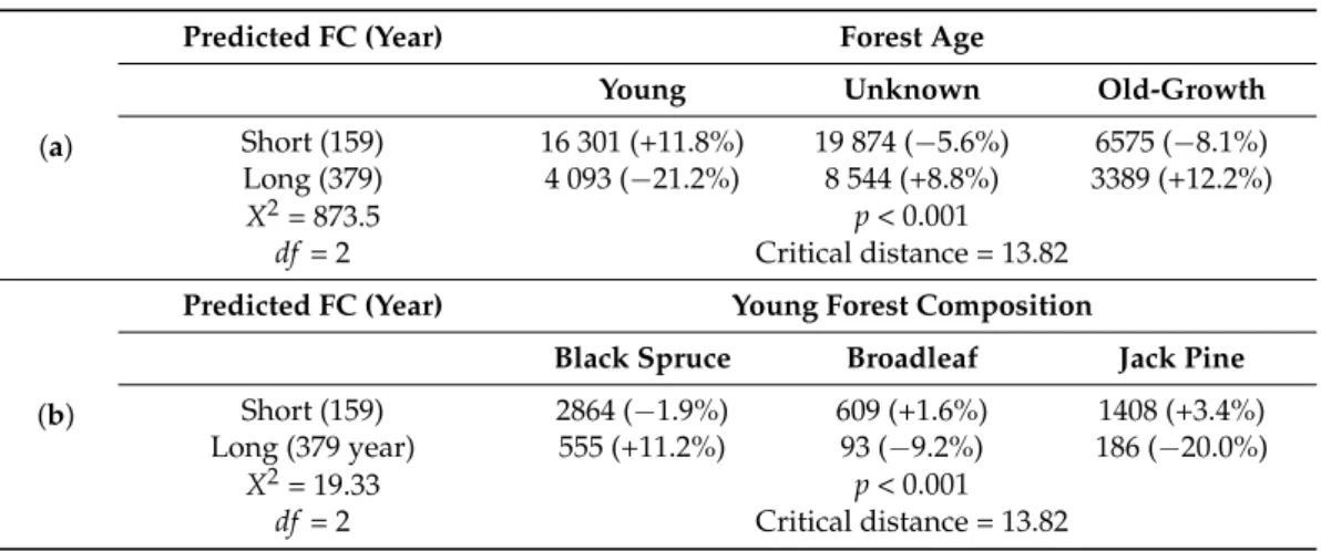
Pearson’s chi-square test confirms that age-structure is younger where FC is short. The Freeman–Tukey deviate shows that each observed deviance is significant (p < 0.001) (Table6a). Young forests compose 38% of short FC zones, which is 11.8% more than expected from a homogeneous distribution. They compose 26% of long FC zones, which is 20% less abundant than expected from a homogeneous distribution. We did not perform statistics on old-growth forest distribution because for certain types of vegetation composition, it was impossible to distinguish mature from old-growth forests. However, both old-growth and unknown age classes were underrepresented in short FC zones (respectively 15% and 46%) and overrepresented in long FC zones (respectively 21% and 46%). 3.5. FC and Succession Pathways
Pearson’s chi-square test confirms that there are differences in the composition of young forests according to FC (Table6b). In short FC zones, 59% of young forests are pure black spruce stands; broadleaf species are present in 12% and jack pine in 29%. In long FC zones, 67% of young forests are pure black spruce stands; broadleaf species are present in 11% and jack pine in 22%. Jack pine is especially rare (´20% less than expected for a random distribution) among young forests in the long FC zones.
Table 6.Contingency tables and chi-square (X2) test of observed frequencies and their deviance from expected frequencies (in parentheses) for (a) young, unknown (mature or old-growth) and old-growth forest types and (b) young forest compositions in short and long FC areas.
(a)
Predicted FC (Year) Forest Age
Young Unknown Old-Growth
Short (159) 16 301 (+11.8%) 19 874 (´5.6%) 6575 (´8.1%) Long (379) 4 093 (´21.2%) 8 544 (+8.8%) 3389 (+12.2%)
X2= 873.5 p < 0.001
df = 2 Critical distance = 13.82
(b)
Predicted FC (Year) Young Forest Composition
Black Spruce Broadleaf Jack Pine
Short (159) 2864 (´1.9%) 609 (+1.6%) 1408 (+3.4%) Long (379 year) 555 (+11.2%) 93 (´9.2%) 186 (´20.0%)
X2= 19.33 p < 0.001
df = 2 Critical distance = 13.82
4. Discussion
4.1. FC Physical Drivers and Scales
Results show that physical environment influences local FC length. As hypothesized, FC is shorter where soil drainage is locally high (Orders 1–3) and river density is low (Orders 1, 2). Contrary to the original hypothesis, landscape terrain complexity (Orders 4, 5) is positively associated with short FC. In the study area, terrain complexity arises along rivers, which are both associated with sandy deposits and rocky outcrops. Contrary to the initial hypothesis, topographic features may not act as fire breaks, but rather, as fire corridors. Riverbeds are embedded in rocky outcrops and covered by
Forests 2016, 7, 139 12 of 21
sandy and dry soils, which may contribute to combustible flammability and fire propagation in wind corridors [44,45]. We also observed that landscape slope position (Order 4) is associated with long FC, meaning valleys burn more than hills, which may act as fire breaks [25,73].
Our results show the importance of bottom-up controls on FC in the study area. Similar phenomena are observed in many fire-prone ecosystems (e.g., [48,74–76]), but findings remain scarce for the boreal forest. Some studies highlight the association between FC and local soil drying potential [47,48,68,77], fire-break configuration [34] and topography [30,46,78], while others did not find any or very low bottom-up controls on fire frequency (e.g., [31,79]). As proposed by [76], the lack of consistency between results may be due to different sensitivities depending on FC. The longer FC is, the more influence bottom-up controls should have [29,80]. In another vein, we observed that we can miss some variable effects if we measure them at the wrong scale. We thus argue that single-scale approaches may not be suitable for observing both bottom-up and top-down controls [81,82]. The study area division according to watershed and river orders performed well with identifying FC drivers and their optimal measurement scales.
4.2. A Local FC Model
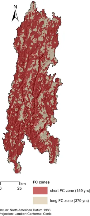
We built a spatially-explicit and scale-relevant FC model, driven by local physical factors. Model selection based on AICc allowed us to order models from the best to the worst with little ambiguity. We first expected to build a multi-scale model whose performance would include different drivers measured at their optimal scale. However, from the pool of possible models,∆AICc indicated a good performance from a model based solely on the local scale for both HD and DRY variables. We identified two possible explanations for the better performance at the local scale. First, local FC could be bottom-up controlled, primarily influenced by local environment. This idea is however not in accordance with the generally accepted idea that fire regimes are driven by top-down, regional factors [78,83]. In that sense, we acknowledge that top-down drivers provide regional trends of FC, but we can argue that local physiography creates non-negligible variability. The second explanation concerns a suspected low performance of landscape-scale watersheds to fit landscape physiography compared to local-scale watersheds. We observe that short and long FC local-scale watersheds are aggregated in patches (Figure7). We thus understand that local measurement of variables is the best to predict FC according to our scaling design, but this is not interpreted as the absence of coarser scale patterns.
Two fire regimes co-occur in the study area, as shown by the bimodal distribution of predicted FC. Heterogeneity in FC distribution can be caused either by temporal or spatial variability in FC. If only temporal variations occurred, FC would be randomly distributed throughout the study area, and no spatial patterns could be observed. However, we observe that zones where fires are frequent follow latitudinal valleys, while zones where fires are rare are mainly concentrated in inter-valley corridors (Figure7). As observed by [44], valleys in this region may be prone to fire because dry deposits follow riverbeds, whose orientation goes along with wind direction, enhancing combustible drought and fire propagation.
4.3. Model Validation
Predicted zones of short and long FC were validated with independent vegetation data. Landscape age-structure theoretically fits a negative exponential distribution whose scaling depends on FC [16]. Following this rule, young forests (TSF < 100 years) should account for 47% of the short FC zone (FC = 159 years) and for 23% of the long FC zone (FC = 379 years). We have observed more abundant young forests where predicted FC is short (vegetation maps from the 1980s [52]), but young forests are still less abundant than expected (38%). We explain this gap by the fire occurrence temporal pattern. Large fires are not equally distributed in time, but occur in some decades of fire-prone weather [21]. Landscape age-structure thus changes in steps, facing significant rejuvenation following fire decades and getting gradually older until the next one. Considering that when vegetation data were collected,
Forests 2016, 7, 139 13 of 21
there had been no large fires in the study area since the 1920s, we assume that the 1980s landscape was more at the end than at the beginning of this continuum.
Forests 2016, 7, 139 13 of 22
Figure 7. Predicted FC spatial distribution as presented in Figure 6b, grouped into short (159 years)
and long (379 years) FC zones. Topography is presented in background hillshade.
4.4. FC and Vegetation
The initial hypothesis that jack pine, a pioneer fire‐dependent species [38,84], is restricted to zones of short FC is only partly verified. Jack pine is more abundant where FC cycle is short, but is not excluded from zones where FC is long. Theory says jack pine should be restricted to sectors where FC < 220 years [18]. In the whole study area, mean FC is 224 years, and most burned areas are attributable to rare and large fires (>10,000 ha), so the time lapse between fires may be too long to sustain an abundant jack pine population. We thus suspect short FC zones to be a reservoir of jack pine during prolonged periods without fire. When large fires occur, jack pine may spread outside short FC zones, helped by post‐fire colonization adaptations such as seed abundance and dispersal, fast growth and serotinous cones [38,85,86]. Paleo‐ecological researchers [33,87] observed a stable jack pine and black spruce local co‐occurrence during the Holocene. Their relative abundance depends on time elapsed since last fire. We suspect this stable co‐occurrence is specific to short FC zones. Further research is needed to investigate local composition changes during the Holocene along a local FC gradient.
Figure 7.Predicted FC spatial distribution as presented in Figure6b, grouped into short (159 years) and long (379 years) FC zones. Topography is presented in background hillshade.
4.4. FC and Vegetation
The initial hypothesis that jack pine, a pioneer fire-dependent species [38,84], is restricted to zones of short FC is only partly verified. Jack pine is more abundant where FC cycle is short, but is not excluded from zones where FC is long. Theory says jack pine should be restricted to sectors where FC < 220 years [18]. In the whole study area, mean FC is 224 years, and most burned areas are attributable to rare and large fires (>10,000 ha), so the time lapse between fires may be too long to sustain an abundant jack pine population. We thus suspect short FC zones to be a reservoir of jack pine during prolonged periods without fire. When large fires occur, jack pine may spread outside short FC zones, helped by post-fire colonization adaptations such as seed abundance and dispersal, fast growth and
Forests 2016, 7, 139 14 of 21
serotinous cones [38,85,86]. Paleo-ecological researchers [33,87] observed a stable jack pine and black spruce local co-occurrence during the Holocene. Their relative abundance depends on time elapsed since last fire. We suspect this stable co-occurrence is specific to short FC zones. Further research is needed to investigate local composition changes during the Holocene along a local FC gradient.
Our results suggest disturbance regime heterogeneity allows different habitats to co-occur in the study area and thus contribute to species diversity. Jack pine is adapted to short FC [86]. It is abundant in western Quebec where FC is generally short and rare in eastern Quebec where FC is long [88]. On the other hand, balsam fir is a shade-tolerant late-succession species [17,89] generally associated with long FC, such as in eastern Quebec [90,91]. Both species are abundant throughout the study area, located in central Quebec [39].
Broadleaf species distribution, although associated with fire frequency [92], was not analyzed because it is mainly restricted to the southern extreme of the study area.
4.5. Implications for Forest Management
FC spatial heterogeneity challenges the scale at which forest management is planned. Ecosystem-based management inspired by natural disturbance regimes aligns harvest rates with historical FC and associated age-structures [12,35,93]. While we showed that fire regime is locally variable, forest management and harvest rates are mostly planned at the landscape or management unit scale [94]. Moreover, depending on available data, FC may be only available for an even wider scale or for a neighboring area (e.g., [61,95]). We found that FC is complex and heterogeneous at a smaller scale than management units.
We argue for the consideration of local FC variability in forest ecosystem management. Different issues affect different locations in a single management unit. On the one hand, zones where FC is short are especially vulnerable to the expected increase in fire frequency due to climate change (e.g., [17,96,97]). The resilience of these forests should be a main management concern, as successive disturbances lead closed forests to turn into open lichen woodlands [98–101]. On the other hand, zones where FC is long face issues associated with old-growth forest depletion, due to a shorter time lapse between harvests than between natural fires [21,22,102]. Strategies for old-growth preservation, such as conservation zones [103], extended harvest rotation time [104] and adapted cutting designs for old-growth structure maintenance [105], should thus be concentrated in long FC zones.
5. Conclusions
FC is widely used for the basic description of boreal forest ecology and has a crucial place in ecosystem management. However, FC relies on the assumption that fire hazard is homogeneous throughout the region of interest. In this research, we demonstrated that homogeneity should not be systematically presumed, and we adapted the FC concept to make it relevant also for heterogeneous regions.
Ecological functions of the patchwork landscape structure and interactions between short and long FC zones remain unknown, although we expect them to contribute to forest diversity and resilience. Each zone may act as a reservoir of species adapted to specific fire intervals, such as jack pine in short FC zones and balsam fir in long FC zones. This may enhance the adaptation potential to changes in the fire regime and, subsequently, to climate change.
Finally, our results suggest that FC drivers are scale dependent, so we argue for further consideration of scale issues in fire regime studies. Research in the area of FC spatial heterogeneity is needed to address the question of the mechanisms involved. In that sense, comparing the results from statistical models as we did and from fire behavior models is an interesting avenue to explore. Assessing the heterogeneity of other parameters of fire regimes, such as ignition patterns and fire severity, could also provide useful insights.
Forests 2016, 7, 139 15 of 21
Acknowledgments: We greatly thank Élisabeth Turcotte, Myriam Jourdain, David Gervais, Léa Langlois, Alexandre Turcotte, Nicolas Fauvart, Jean-Guy Girard, as well as Université du Québec à Chicoutimi plant ecology lab members for their assistance in the lab and in the field. We thank Aurélie Terrier for revising the manuscript and the anonymous reviewers for their helpful comments. We also acknowledge the Natural Sciences and Engeneering Research Council of Canada-UQAT-UQAM Industrial Chair in Sustainable Forest Management for material and scientific support. This project was funded by the Fonds de la Recherche Forestière du Saguenay-Lac-Saint-Jean and the Fonds de Recherche Nature et Technologies du Québec. We used forest inventory and fire data from the ministère des Ressources naturelles et de la Faune du Québec. We also acknowledge the financial contribution of the Natural Sciences and Engineering Research Council of Canada. Finally, we thank Resolute Forest Products for their partnership in the project and accommodation during field work.
Author Contributions:H.M., S.G. and Y.B. conceived of and coordinated the research project. A.C.B. and S.G. designed data collection. A.C.B. and M.D. conceived of the cartography tools. N.M. provided support for the surficial deposits classification. A.C.B. and A.L. analyzed the data. A.C.B. wrote the paper. All authors revised it.
Conflicts of Interest:The authors declare no conflicts of interest.
Abbreviation
The following abbreviations are used in this manuscript: FC Fire cycle
TSF Time since last fire
DRY Dry surficial deposit density HD Hydrographic density ESD Elevation standard deviation TPI Topographic position index Appendix Forests 2016, 7, 139 15 of 22 acknowledge the financial contribution of the Natural Sciences and Engineering Research Council of Canada. Finally, we thank Resolute Forest Products for their partnership in the project and accommodation during field work. Author Contributions: H.M., S.G. and Y.B. conceived of and coordinated the research project. A.C.B. and S.G. designed data collection. A.C.B. and M.D. conceived of the cartography tools. N.M. provided support for the surficial deposits classification. A.C.B. and A.L. analyzed the data. A.C.B. wrote the paper. All authors revised it. Conflicts of Interest: The authors declare no conflicts of interest. Abbreviation The following abbreviations are used in this manuscript: FC Fire cycle TSF Time since last fire DRY Dry surficial deposit density HD Hydrographic density ESD Elevation standard deviation TPI Topographic position index Appendix
Figure A1. Rivers’ Strahler order (1–4) inside an Order 4 watershed. Order 1 rivers connecting
together make an Order 2 river; Order 2 rivers connecting together make an Order 3 river, etc.
Figure A1.Rivers’ Strahler order (1–4) inside an Order 4 watershed. Order 1 rivers connecting together make an Order 2 river; Order 2 rivers connecting together make an Order 3 river, etc.
Forests 2016, 7, 139 16 of 21
Forests 2016, 7, 139 16 of 22
Figure A2. Coefficient and confidence intervals (calculated with bootstrap) plots of variables ln(DRY + 1), HD, ESD and TPI, Orders 1–5, for univariate Cox
regressions. TSF data describe the study area age‐structure as it was in 2010 (shaded rectangle, as used for analysis), 2009, 2006 and 2004. Order 1 ye ar -2 -1 0 1 2 2004 200 7 2010 ln(DRY+1) Order 2 -2 -1 0 1 2 Order 3 -2 -1 0 1 2 Order 4 -2 -1 0 1 2 Order 5 -2 -1 0 1 2 ye ar -0.2 -0.1 0.0 0.1 0.2 2004 2007 201 0 HD -0.2 -0.1 0.0 0.1 0.2 -0.2 -0.1 0.0 0.1 0.2 -0.2 -0.1 0.0 0.1 0.2 -0.2 -0.1 0.0 0.1 0.2 ye ar -0.02 -0.01 0.00 0.01 0.02 2004 200 7 2010 ESD -0.02 -0.01 0.00 0.01 0.02 -0.02 -0.01 0.00 0.01 0.02 -0.02 -0.01 0.00 0.01 0.02 -0.02 -0.01 0.00 0.01 0.02 ye ar -0.4 -0.2 0.0 0.2 0.4 20 04 2007 201 0 TPI -0.4 -0.2 0.0 0.2 0.4 coefficient -0.4 -0.2 0.0 0.2 0.4 -0.4 -0.2 0.0 0.2 0.4 -0.4 -0.2 0.0 0.2 0.4
Figure A2.Coefficient and confidence intervals (calculated with bootstrap) plots of variables ln(DRY + 1), HD, ESD and TPI, Orders 1–5, for univariate Cox regressions. TSF data describe the study area age-structure as it was in 2010 (shaded rectangle, as used for analysis), 2009, 2006 and 2004.
Forests 2016, 7, 139 17 of 21
Table A1.Model comparisons based on AICc. Results for the 15 candidate models (∆AICc < 2) are
presented. The selected model is shaded.
Model Degrees of Freedom Loglikelihood AICc ∆AICc Weight
1 log(DRY1) + log(DRY3) + HD1 3 ´357.8589 721.8892 0.0000 0.0575
2 log(DRY3) + HD1 + ESD1 3 ´357.8718 721.9151 0.0259 0.0568
3 log(DRY1) + log(DRY3)3 + HD1 + ESD1 4 ´356.8615 722.0108 0.1217 0.0541
4 log(DRY1) + HD1 + ESD3 3 ´358.1568 722.4850 0.5958 0.0427
5 log(DRY1) + HD1 2 ´359.2333 722.5517 0.6626 0.0413
6 log(DRY1) + log(DRY3) + HD1 + ESD3 4 ´357.1722 722.6322 0.7430 0.0397
7 log(DRY1) + log(DRY3) + HD1 + TPI4 4 ´357.3373 722.9624 1.0732 0.0336
8 log(DRY3) + HD1 + ESD1 + TPI4 4 ´357.4987 723.2851 1.3959 0.0286
9 log(DRY1) + HD1 + TPI4 3 ´358.5942 723.3597 1.4706 0.0276
10 log(DRY1) + log(DRY3) + HD1 + ESD1 + TPI4 5 ´356.5770 723.5888 1.6997 0.0246
11 log(DRY1) + HD1 + ESD3 + TPI4 4 ´357.7217 723.7312 1.8421 0.0229
12 log(DRY3) + HD1 + HD3 + ESD1 4 ´357.7719 723.8315 1.9423 0.0218
13 log(DRY1) + HD1 + ESD1 3 ´358.8381 723.8476 1.9584 0.0216
14 log(DRY3) + HD1 + ESD1 + ESD3 4 ´357.7942 723.8762 1.9870 0.0213
15 log(DRY1) + log(DRY3) + HD1 + HD3 4 ´357.8120 723.9117 2.0225 0.0209
Steps for watershed computation from a digital elevation model (20 m resolution). Hydrology tools in ArcGIS are indicated in italics. 1. Fill; 2. Flow direction; 3. Identify streams: Reclass, >16 ha = 1; 4. Snap Pour points + edit pour points by visual inspection; 5. Stream order (Strahler); Order 1 is excluded for fuzziness; 6. Compute Watersheds separately for all Strahler orders; 7. Visual inspection and corrections if needed (e.g., one cell watersheds).
References
1. Bonan, G.B.; Shugart, H.H. Environmental factors and ecological processes in boreal forests. Annu. Rev. Ecol. Syst. 1989, 20, 1–28. [CrossRef]
2. Payette, S. Fire as a controlling process in the North American boreal forest. Syst. Anal. Glob. Boreal For. 1992, 144–169. [CrossRef]
3. Stocks, B.J.; Mason, J.A.; Todd, J.B.; Bosch, E.M.; Wotton, B.M.; Amiro, B.D.; Flannigan, M.D.; Hirsch, K.G.; Logan, K.A.; Martell, D.L.; et al. Large forest fires in Canada, 1959–1997. J. Geophys. Res. 2003, 108, 1–12. [CrossRef]
4. Johnson, E.A. Fire and Vegetation Dynamics: Studies from the North American Boreal Forest; Cambridge University Press: Cambridge, UK, 1992; p. 129.
5. Bergeron, Y.; Gauthier, S.; Kafka, V.; Lefort, P.; Lesieur, D. Natural fire frequency for the eastern Canadian boreal forest: Consequences for sustainable forestry. Can. J. For. Res. 2001, 31, 384–391. [CrossRef]
6. Wu, J.; Loucks, O.L. From balance of nature to hierarchical patch dynamics: A paradigm shift in ecology. Q. Rev. Biol. 1995, 70, 439–466. [CrossRef]
7. Dix, R.L.; Swan, J.M.A. The roles of disturbance and succession in upland forest at Candle Lake, Saskatchewan. Can. J. Bot. 1971, 49, 657–676. [CrossRef]
8. Landres, P.B.; Morgan, P.; Swanson, F.J. Overview of the use of natural variability concepts in managing ecological systems. Ecol. Appl. 1999, 9, 1179–1188.
9. Gauthier, S.; Vaillancourt, M.-A.; Kneeshaw, D.D.; Drapeau, P.; de Grandpré, L.; Claveau, Y.; Paré, D. Forest Ecosystem Management: Origins and Foundations. In Ecosystem Management in the Boreal Forest; Gauthier, S., Vaillancourt, M.-A., Leduc, A., de Grandpré, L., Kneeshaw, D.D., Morin, H., Drapeau, P., Bergeron, Y., Eds.; Les Presses de l’Université du Québec: Quebec, QC, Canada, 2009; pp. 13–38.
10. Gauthier, S.; Leduc, A.; Bergeron, Y. Forest dynamics modelling under natural fire cycles: A tool to define natural mosaic diversity for forest management. Environ. Monit. Assess. 1996, 39, 417–434. [CrossRef] [PubMed]
11. Kuuluvainen, T. Natural variability of forests as a reference for restoring and managing biological diversity in boreal Fennoscandia. Silva Fenn. 2002, 36, 97–125. [CrossRef]
12. Franklin, J.F.; Spies, T.A.; Pelt, R.V.; Carey, A.B.; Thornburgh, D.A.; Berg, D.R.; Lindenmayer, D.B.; Harmon, M.E.; Keeton, W.S.; Shaw, D.C.; et al. Disturbances and structural development of natural forest ecosystems with silvicultural implications, using Douglas-fir forests as an example. For. Ecol. Manag. 2002, 155, 399–423. [CrossRef]
13. Gauthier, S.; Raulier, F.; Ouzennou, H.; Saucier, J.-P. Strategic analysis of forest vulnerability to risk related to fire: An example from the coniferous boreal forest of Quebec. Can. J. For. Res. 2015, 45, 553–565. [CrossRef]
![Figure 1. Stand origin map [21] within the study area, including fire delineation (1900–2010) from aerial photos and time elapsed since last fire (TSF) sampling points.](https://thumb-eu.123doks.com/thumbv2/123doknet/7657995.238219/3.892.278.606.593.1079/figure-stand-origin-within-including-delineation-elapsed-sampling.webp)