ÉCOLE DE TECHNOLOGIE SUPÉRIEURE UNIVERSITÉ DU QUÉBEC
THESIS PRESENTED TO
ÉCOLE DE TECHNOLOGIE SUPÉRIEURE
IN PARTIAL FULFILLEMENT OF THE REQUIREMENTS FOR THE DEGREE OF DOCTOR OF PHILOSOPHY
Ph.D.
BY Yan ZHAO
INVESTIGATION OF UNCERTAINTIES IN ASSESSING CLIMATE CHANGE IMPACTS ON THE HYDROLOGY OF A CANADIAN RIVER WATERSHED
MONTREAL, JULY 21 2015
This Creative Commons licence allows readers to dowload this work and share it with others as long as the author is credited. The content of this work can’t be modified in any way or used commercially.
BOARD OF EXAMINERS
THIS THESIS HAS BEEN EVALUATED BY THE FOLLOWING BOARD OF EXAMINERS
Mr. Robert Leconte, Thesis Supervisor
Department of Civil Engineering, Université de Sherbrooke
Mr. Robert Benoit, President of the Board of Examiners
Department of Mechanical Engineering, École de technologie supérieure
Mr. François Brissette, Member of the jury
Department of Construction Engineering, École de technologie supérieure
Mrs. Annie Poulin, Member of the jury
Department of Construction Engineering, École de technologie supérieure
Mr. Alain N. Rousseau, External Evaluator
Institut national de la recherche scientifique, Centre Eau, Terre et Environnement
THIS THESIS WAS PRESENTED AND DEFENDED
IN THE PRESENCE OF A BOARD OF EXAMINERS AND PUBLIC ON JUNE 16 2015
FOREWORD
This PhD research started in May 2008 at the École de technologie supérieure, Université du Québec, under the supervision of Professor Robert Leconte, now at the Université de Sherbrooke. This thesis is part of the project entitled “Impact of climate change in Canadian River Basins and adaptation strategies for the hydropower industry”, which was supported by the Natural Science and Engineering Research Council of Canada (NSERC), Hydro-Québec, Manitoba Hydro and the Ouranos Consortium on Regional Climatology and Adaptation Climate Change.
ACKNOWLEDGMENT
Upon writing this thesis, many emotions came to me. Throughout these years of my life, I have encountered many dilemmas and also received many help. I am very grateful for all the people who supported me, encouraged me and provided me with advice and suggestions in the course of my research. Without them, I cannot imagine how I could have made this achievement.
First of all, I would like to express my particularly appreciation and thanks to my supervisor, Prof. Robert LECONTE. Since I came to Canada, I have received countless help and support from you. Even after you moved to the University of Sherbrooke, you continued supervising my research work. Your serious and responsible attitude in scientific research greatly impressed me. And your modesty and optimism in daily communications also deeply touched me. When I felt trapped in my research, you helped me to find solutions; when I was homesick, your words gave me great comfort; when I felt tired and frustrated in dealing with technical problems, you were a good advisor who gave me much encouragement and cheered me up. During these years of PhD research, you were not only a research supervisor to me, but also a close friend and a reliable mentor. Your powerful support encouraged me to complete my PhD study. I very much appreciated your years of guidance and help.
Secondly, I would like to thank another important advisor in ÉTS, Prof. François P. BRISSETTE. You possess a wealth of knowledge and also a rigorous working attitude. You have vast interests and can easily entertain a pleasant conversation. You helped me discovering uncertain points and gave me sound advice in my research. Since my supervisor left ÉTS, you were always concerned about my studies, providing help when needed. I appreciate what you have done for me. I am also very grateful to Prof. Annie POULIN who gave me great assistance in applying the hydrological model HYDROTEL in my research and provided me with numerous helpful ideas. You are a very nice and intelligent professor. Thank you.
I am extremely grateful to all the members of the jury who evaluated my thesis. Your comments were very important to me to enhance this work.
This PhD research was also supported by scientists at Hydro-Québec and at the Ouranos Consortium: Marie Minville, Blaise Gauvin St-Denis and Diane Chaumont. Thank you all for giving me valuable expertise and providing me important technical information. Your sensible suggestions prompted me to find a way out. Heartily thank you.
I would like to thank the following persons with whom I had the privilege of working alongside, or interacted with, during these years I was doing my PhD study: postdoctoral colleague Jie CHEN (École de technologie supérieure, Canada), postdoctoral colleague Zhi LI (North West Agriculture and Forestry University, China), postdoctoral colleague Mélanie TRUDEL (Université de Sherbrooke, Canada), postdoctoral colleague Didier HAGUMA (Université de Sherbrooke, Canada), PhD student Richard ARSENAULT (École de technologie supérieure, Canada), Master student Jean-Luc MARTEL (École de technologie supérieure, Canada), as well as students who graduated including Johnathan ROY, Chloé ALASSIMONE, Josée BEAUCHAMP, Anne-Sophie PRUVOST, Pascal CÔTÉ, Jean Stéphane MALO, Antonin COLADON and Sébastien TILMANT. Thanks to you, my PhD study was anything but humdrum and painful. It was so pleasing to work with these joyful peoples. Special thanks to Didier HAGUMA who helped me working with the hydrological model SWAT, provided the NLWIS data and the geographical information of the Manicouagan River Basin. I sincerely thank these enthusiastic colleagues. They gave me many valuable comments and suggestions. My research is inseparable from the cooperation and assistance of this group.
Thanks to the secretaries and librarians at the École de technologie supérieure, for helping me in many different ways. Thank you to Lise DAIGNEAULT and Dominique CHARRON at the Décanat des études for explaining academic issues. Thank you, Mathieu DULUDE, for helping me to resolve the computer-related technical problems.
I would also like to express my appreciation to my dear friends: Master student Yingying DONG (École de technologie supérieure, Canada), PhD student Jing LI (McGill University, Canada), MBA student Wei XUE (Concordia University, Canada), Dr. Xing CHEN (Hohai University, China) and Dr. Qin XU (Nanjing Hydraulic Research Institute, China). When I was homesick and sad, you gave me encouragement, straightened me out and helped me to overcome difficulties and concentrate on my study. You were my spiritual support.
Most importantly, I am deeply indebted to my family for all their help. Especially, thanks to my parents, my older brother, my sister-in-law and my niece. Since I left home to pursue my study in France in 2006, I spent very limited time to see them. They always comforted me to focus on my study. When I worried about my parents, my brother and sister-in-law appeased while taking good care of them. I am grateful that my family understands me, supports me and loves me unconditionally. Their encouragement inspired me to persevere in my objective for so long. Especially, I would like to thank an important person in my life, Yaochi ZHANG. It is him who encouraged me to come to Canada to do my PhD research. He always shared my worries; let me feel at ease when we were separated on different continents. I found serenity because he is always besides me at any time.
Great thanks to the organizations for providing financial support for this project: the Natural Science and Engineering Research Council of Canada (NSERC), Hydro-Québec, Manitoba Hydro and the Ouranos Consortium.
Finally, I want to express endless thanks to all the people who made this thesis possible, those who are mentioned above and those who are not. This thesis owes to your support. Thank you very much!
INVESTIGATION OF UNCERTAINTIES IN ASSESSING CLIMATE CHANGE IMPACTS ON THE HYDROLOGY OF A CANADIAN RIVER WATERSHED
Yan ZHAO
ABSTRACT
It is known that climate change will affect water resources. The impact of climate change on river regimes attracted the attention of hydropower companies over the recent years. Although general trends in future river flows can be reasonably well assessed using climate and hydrological models, their overall uncertainty is much more difficult to evaluate. An improved evaluation of uncertainty in the hydrological response of watersheds to climate change would help designing hydropower projects as well as adapting existing systems to better cope with the anticipated changes in flow regimes.
The uncertainty in assessing the potential hydrological impacts of a changing climate is of high interest for the scientific community. A framework for evaluating the uncertainty of climate change impacts on watershed hydrology is developed in this thesis. The sources of uncertainty studied comprise the global climate model (GCM) structure, climate sensitivity, natural variability and, to a lesser extent, hydrological model structure. Climate sensitivity is the global mean climatological temperature change due to a doubling of atmospheric CO2 concentration. Natural variability refers to the uncertainties resulting from the inherent randomness or unpredictability in the natural world. Climate projections under IPCC A2 scenario for the 2080 horizon were downscaled to regional scale using the change factor method and developed into long time series with WeaGETS, a stochastic weather generator developed at the École de technologie supérieure. The predicted future climate scenarios were forced into four hydrological models to simulate future flows in the Manicouagan River Basin, located in the province of Quebec, Canada. The Monte Carlo sampling method was implemented as a probabilistic approach to trace out the magnitude of uncertainty in accordance with the weighting schemes attributed to the different sources of uncertainty. In particular, equal and unequal weights were attributed to the GCMs to see whether this would have a significant impact on the resulting flow return periods. This experiment was motivated by the fact that GCM structure is usually the most significant contribution to the overall uncertainty in projected flows. Experiments using equal and unequal weights on climate sensitivities were also performed.
Modelling results indicate that the future hydrological cycle will intensify as precipitation and temperature will increase in the future for all GCMs projections. The spring peak flow will occur earlier by a few weeks for all GCMs investigated and will increase for a majority of them.
The uncertainty related to GCM structure, climate sensitivity, natural variability and to hydrological model structure were assessed separately. Uncertainty due to the GCM structure
was found to be significant and to vary seasonally and monthly especially during the month of April. Variations in climate sensitivity and natural variability introduced moderate changes in the hydrological regime when compared with the uncertainty due to GCM structure. The choice of hydrological model will also result in a non-negligible uncertainty in climate change studies.
At last, the magnitude of uncertainty under various weighting schemes attributed to GCMs and climate sensitivities was evaluated. Weight scheme experiments indicate that assigning equal or unequal weights to the GCM structure had a marginal to small effect on the return periods calculated for the hydrological variables studied, i.e. monthly discharge and spring runoff volume. However, for climate sensitivity, the weights assignment notably influenced the probability of occurrence of large hydrological events. The choice of the hydrological model also had a significant impact on return periods of large hydrological events. It should be given due attention in selecting hydrological models and assigning weights on climate sensitivities in uncertainty assessment of climate change impacts in designing water resources systems.
Keywords: climate change, uncertainty, impact, hydrology, climate sensitivity, Monte Carlo method
ÉTUDE DES INCERTITUDES ASSOCIÉES À L’ÉVALUATION DE L’IMPACT DES CHANGEMENTS CLIMATIQUES SUR L’HYDROLOGIE D’UN BASSIN
VERSANT CANADIEN Yan ZHAO
SUMMARY
Il est connu que le changement climatique aura une incidence sur les ressources en eau. L'impact du changement climatique sur les régimes hydriques a attiré l'attention des entreprises hydroélectriques au cours des dernières années. Bien que les tendances générales dans les débits en rivière puissent être raisonnablement bien évaluées à l'aide des modèles climatiques et hydrologiques, leur incertitude globale est beaucoup plus difficile à quantifier. Une meilleure évaluation de l'incertitude de la réponse hydrologique des bassins versants aux changements climatiques permettrait la conception de projets hydroélectriques ainsi que l'adaptation des systèmes existants afin de mieux faire face aux changements prévus dans les régimes d'écoulement.
L'incertitude dans l'évaluation des impacts hydrologiques potentiels du changement climatique est d‘un grand intérêt pour la communauté scientifique. Une méthodologie pour l'évaluation de l'incertitude des impacts du changement climatique sur l'hydrologie des bassins versants est développée dans cette thèse. Les sources d’incertitudes étudiées comprennent la structure des modèles de climat global (MCG), la sensibilité du climat, la variabilité naturelle du climat et, dans une moindre mesure, la structure du modèle hydrologique. La sensibilité du climat est le changement de la température climatologique moyenne mondiale en raison d'un doublement de la concentration de CO2 dans l'atmosphère. La variabilité naturelle réfère aux incertitudes résultant de l'aléa inhérent ou imprévisibilité dans le monde naturel. Les projections climatiques dans le scénario A2 du GIEC pour l'horizon 2080 ont été réduites à l'échelle régionale par une méthode du facteur de changement et développées en longues séries chronologiques avec le générateur météorologique WeaGETS conçu à l’École de technologie supérieure. Les scénarios climatiques futurs ont été forcés dans quatre modèles hydrologiques pour simuler les débits futurs sur le bassin de la rivière Manicouagan, situé dans la province de Québec, Canada. La méthode d'échantillonnage de Monte Carlo a été mise en œuvre comme approche probabiliste pour établir l'ampleur de l'incertitude en conformité avec les schémas de pondération attribués aux différentes sources d'incertitude. En particulier, des poids égaux et inégaux ont été attribués aux MCG pour voir si cela avait un impact significatif sur les périodes de retour des débits simulés. Cette expérience a été motivée par le fait que la structure des MCG est habituellement la plus importante contribution à l'incertitude globale des débits projetés. Des expériences utilisant des poids égaux et inégaux sur la sensibilité du climat ont également été réalisées.
Les résultats de la modélisation indiquent que le cycle hydrologique futur s'intensifiera à mesure que les précipitations et la température vont augmenter dans l'avenir pour toutes les
projections des MCG. Le débit de pointe du printemps aura lieu plus tôt de quelques semaines pour tous les MCG analysés et va augmenter pour une majorité d'entre eux.
L'incertitude liée à la structure des MCG, à la sensibilité du climat, à la variabilité naturelle et à la structure du modèle hydrologique ont été évalués séparément. L’incertitude due à la structure du MCG a été jugée importante et varie mensuellement, en particulier durant le mois d’avril. Les variations de la sensibilité du climat et de la variabilité naturelle introduisent des changements modérés dans le régime hydrologique, par rapport à l'incertitude due à la structure des MCG. Le choix du modèle hydrologique se traduit également par une incertitude non négligeable dans les études sur le changement climatique. Enfin, l'ampleur de l'incertitude pour différents systèmes de pondération attribués aux MCG et à la sensibilité du climat a été évaluée. Les résultats indiquent que l'attribution de pondérations égales ou inégales à la structure du MCG a un effet marginal à faible sur les périodes de retour calculées pour les variables hydrologiques étudiées, soient le débit mensuel et le volume de ruissellement printanier. Cependant, pour la sensibilité du climat, le schéma de pondération a notamment influencé la probabilité d'occurrence de grands événements hydrologiques. Le choix du modèle hydrologique a également eu un impact significatif sur les périodes de retour de grands événements hydrologiques. Une attention particulière devra donc être accordée quant au choix des modèles hydrologiques et dans l'attribution de pondérations sur la sensibilité du climat, pour l'évaluation de l'incertitude des impacts du changement climatique sur les régimes hydriques.
Mots-clés: changement climatique, incertitude, impact, hydrologie, sensibilité du climat, méthode de Monte Carlo
TABLE OF CONTENTS
Page
INTRODUCTION ...1
CHAPITRE 1 RESEARCH STATEMENT ...5
1.1 Background ...5
1.2 Research statement ...6
1.3 Weight assignment ...9
1.4 Objectives ...10
CHAPITRE 2 LITERATURE REVIEW ...13
2.1 Definition of uncertainty ...13 2.2 Classification of uncertainty ...15 2.2.1 Natural uncertainty ... 15 2.2.2 Model uncertainty ... 16 2.2.3 Parameter uncertainty ... 16 2.2.4 Behavioral uncertainty ... 18 2.2.5 Summary ... 19
2.3 Uncertainty assessment in climate change impacts on hydrological regimes ...19
2.3.1 Uncertainty in climate models ... 21
2.3.2 Uncertainty in climate sensitivity ... 26
2.3.3 Uncertainty in emission scenarios ... 28
2.3.4 Uncertainty in downscaling methods ... 29
2.3.5 Uncertainty in natural variability ... 31
2.3.6 Uncertainty in hydrological modeling ... 32
2.3.7 Multi-source uncertainty assessment and risk analyses ... 35
2.3.7.1 Uniform weighting strategies ... 36
2.3.7.2 Unequal-weight assigning strategies ... 37
CHAPITRE 3 METHODOLOGY ...41
3.1 Research assumptions ...43
3.2 Climate projections ...44
3.2.1 Global climate models ... 45
3.2.2 Climate sensitivity ... 45 3.3 Downscaling ...50 3.4 Natural variability ...51 3.5 Hydrological modeling ...52 3.5.1 Hydrological models ... 53 3.5.1.1 HSAMI model ... 53 3.5.1.2 HMETS model ... 54 3.5.1.3 HYDROTEL model ... 55 3.5.1.4 HBV model ... 56
3.6 Uncertainty assessment ...59
3.6.1 Monte Carlo simulation ... 59
3.6.2 REA method... 63
3.6.3 Frequency analysis ... 67
CHAPITRE 4 STUDY WATERSHED AND DATA ...69
4.1 General watershed description ...69
4.2 Climatological, physiographic, and flow data ...73
4.2.1 Climatological data ... 73
4.2.1.1 NLWIS data ... 73
4.2.1.2 GCM data ... 74
4.2.2 Physiographic data ... 76
4.2.3 Hydrological data ... 77
CHAPTER 5 RESULTS AND DISCUSSION ...79
5.1 Climate projections ...79
5.2 Uncertainty in projected flows ...85
5.2.1 Hydrological model calibration ... 85
5.2.2 Overall uncertainty ... 89
5.2.3 GCM structure ... 93
5.2.4 Climate sensitivity ... 98
5.2.5 Natural variability ... 100
5.2.6 Hydrological model structure ... 101
5.3 Monte Carlo simulation ...105
5.3.1 Annual mean discharge ... 108
5.3.2 Spring peak discharge ... 111
5.4 Discussion ...113
5.4.1 Uncertainty study ... 114
5.4.2 Analysis using a Monte-Carlo simulation... 118
CONCLUSION…. ...121
RECOMMENDATIONS ...127
LIST OF TABLES
Page Table 3.1 Main properties of the hydrological models ... 53 Table 4.1 Characteristics of the main sub-watersheds of the MRB ... 70 Table 4.2 General information on the selected GCM, including the number of grid
points covering the province of Québec and climate sensitivity value ... 74 Table 5.1 The seasonal and annual change (in square brackets) of precipitation
(∆P/P) obtained for each GCM from three climate sensitivities (2.0°C, 3.0°C, 4.0°C) respectively with scenario A2, 2080 time horizon (2065-2097). The ranking of climate sensitivity uncertainty (1: high uncertainty; 10: low uncertainty) for each GCM is presented in parentheses, based on range ... 82 Table 5.2 The seasonal and annual change (in square brackets) of temperature (∆T)
obtained for each GCM from three climate sensitivities (2.0°C, 3.0°C, 4.0°C) respectively with scenario A2, 2080 time horizon (2065-2097). The ranking of climate sensitivity uncertainty (1: high uncertainty; 10: low uncertainty) for each GCM is presented in parentheses, based on
range ... 83 Table 5.3 Nash-Sutcliffe coefficients obtained for four hydrological models by
using flow time series at the daily time step ... 87 Table 5.4 Average annual flows for 2080 time horizon (2065-2097) and relative
increases (%) compared to average annual flows for control period over
the MRB ... 92 Table 5.5 Uncertainty of GCM structure for all four seasons produced by each
hydrological model. Max (%) is the maximum change in median flow,
Min (%) is the minimum change and UC is uncertainty ... 97 Table 5.6 Reliability, performance and convergence factors R, RB and RD from the
REA method used to generate relative weights W for each GCM, based
on precipitation (P) and temperature (T) ... 106 Table 5.7 Various combinations of weights calculated for each GCM ... 107 Table 5.8 Return period (in years) of annual mean discharge simulated by the
HYDROTEL model for different weighting schemes on GCM and climate sensitivity (CS is climate sensitivity, = is equal weight, ≠ is
Table 5.9 Return period (in years) of annual mean discharge simulated by the HBV model for different weighting schemes on GCM and climate sensitivity
(CS, = and ≠ are indicated in Table 5.8) ...110 Table 5.10 Return period (in years) of annual mean discharge simulated by the
HSAMI model for different weighting schemes on GCM and climate
sensitivity (CS, = and ≠ are indicated in Table 5.8) ...110 Table 5.11 Return period (in years) of annual mean discharge simulated by the
HMETS model for different weighting schemes on GCM and climate
sensitivity (CS, = and ≠ are indicated in Table 5.8) ...111 Table 5.12 Return period (in years) of annual spring peak discharge simulated by
the HYDROTEL model for different weighting schemes on GCM and
climate sensitivity (CS, = and ≠ are indicated in Table 5.8) ...112 Table 5.13 Return period (in years) of annual spring peak discharge simulated by
the HBV model for different weighting schemes on GCM and climate
sensitivity (CS, = and ≠ are indicated in Table 5.8) ...112 Table 5.14 Return period (in years) of annual spring peak discharge simulated by
the HSAMI model for different weighting schemes on GCM and climate sensitivity (CS, = and ≠ are indicated in Table 5.8) ...113 Table 5.15 Return period (in years) of annual spring peak discharge simulated by
the HMETS model for different weighting schemes on GCM and climate sensitivity (CS, = and ≠ are indicated in Table 5.8) ...113 Table 5.16 Relative contributions (in percent) of each source of uncertainty (GCM
structure, climate sensitivity and natural variability) to the overall
LIST OF FIGURES
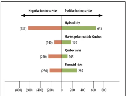
Page Figure 2.1 Analysis of net earnings sensitivity to various risks for 2008 (in millions
of dollars) ... 20
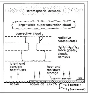
Figure 2.2 Schematic illustration of the GCM structure of an individual land/ocean-atmospheric column ... 22
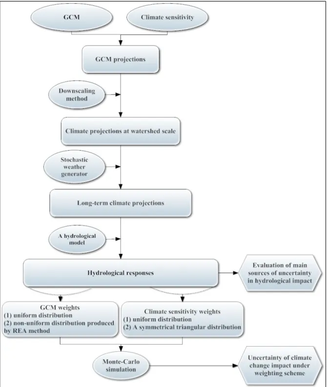
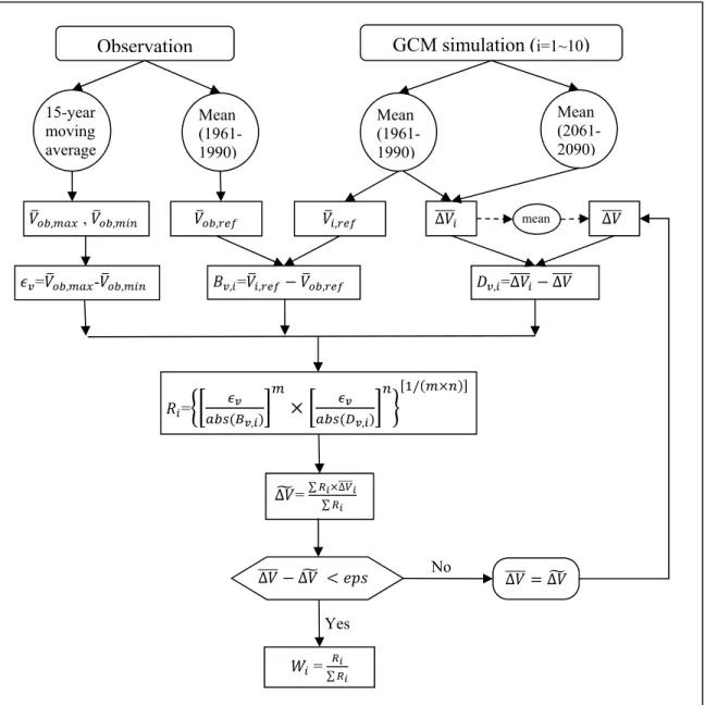
Figure 3.1 Flow chart of the methodology. The flow chart applies to each of the four hydrological models employed in this study ... 42
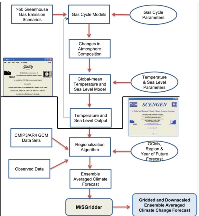
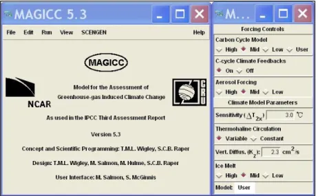
Figure 3.2 Schematic diagram of the structure and flow of the MAGICC/SCENGEN software. The user-defined parameters of the model are displayed in the elliptical shapes ... 48
Figure 3.3 Adjustable forcing controls and climate model parameters in the MAGICC model ... 49
Figure 3.4 Flowchart showing the combination of GCM structure, climate sensitivity and natural variability that was used to produce the precipitation and temperature time series inputted into the hydrological models ... 52
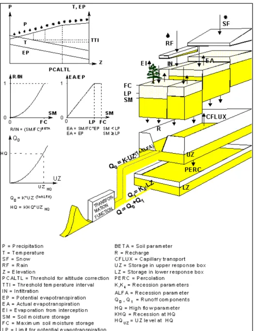
Figure 3.5 Flow chart of the lumped conceptual HSAMI model ... 55
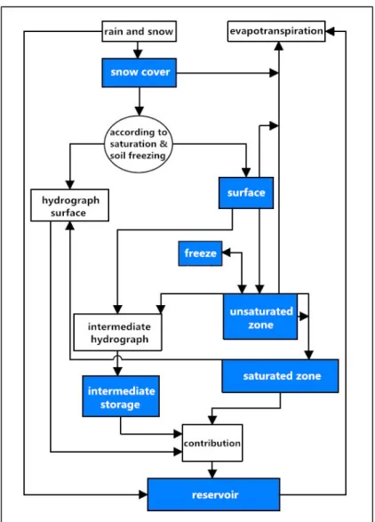
Figure 3.6 Schematic structure of one subbasin in the HBV model... 58
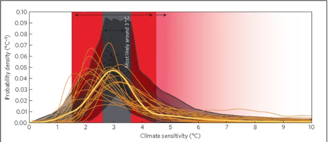
Figure 3.7 Probability density function (PDF) of climate sensitivity. The shaded grey area bounded by a thick black line on the background represents the envelope of all 10,000 randomly drawn climate sensitivity distributions (thin black lines) that are in line with the AR4 climate sensitivity statements. The grey vertical area indicates the most likely probability range around 3.0°C ... 61
Figure 3.8 The triangular probability distribution of climate sensitivity ... 61
Figure 3.9 Graphical representation of Monte Carlo method ... 62
Figure 3.10 REA method implementation scheme ... 65
Figure 4.1 Location map of the Manicouagan basin with its river network of hydroelectric generating stations and main sub-watersheds ... 70
Figure 4.2 Average annual hydrograph of the Manicouagan River Basin at the McCormick station (Manic 1 power station) before (1947-1950) and
after (1976-1979) building the Manicouagan Reservoir ...71 Figure 4.3 Topography and land use in the Manicouagan River Basin ...72 Figure 4.4 Atmospheric CO2 concentrations projected for 6 SRES illustrative
scenarios ...75 Figure 4.5 Average variation in temperature and precipitation in the Manicouagan
River Basin for the 2080 time horizon ...76 Figure 5.1 Scatter plots of seasonal and annual changes of temperature and
precipitation obtained for all ten GCMs and three climate sensitivities (2.0°C, 3.0°C, 4.0°C) with scenario A2 at the 2080 time horizon
(2065-2097). CS represents climate sensitivity ...80 Figure 5.2 Annual average changes of precipitation (left) and temperature (right)
obtained for individual GCMs with five climate sensitivities (2.0°C, 2.5°C, 3.0°C, 3.5°C, 4.0°C) by using scenario A2 at the MRB’s 2080
time horizon (2065-2097) ...85 Figure 5.3 Average annual hydrographs generated by four hydrological models at
the outlet of MRB under recent past climate conditions: (a) calibration period; (b) validation period. The hydrograph of observation is plotted
for comparison ...88 Figure 5.4 Standard deviation of annual discharge generated by four hydrological
models at the outlet of MRB under recent past climate conditions: (a) calibration period; (b) validation period. The hydrograph of observation
is plotted for comparison ...88 Figure 5.5 Envelopes of annual hydrographs and the corresponding changes in
percentage of daily discharge that are simulated in (a) HYDROTEL, (b) HBV, (c) HSAMI and (d) HMETS by using all selected GCMs, climate sensitivities and natural variability at the outlet of MRB for the 2080 horizon (2065-2097). The hydrograph for the control period (1975-2007), which is derived from the corresponding hydrological model’s
simulation, is plotted for the purpose of comparison ...91 Figure 5.6 Box plots of percent of change in average seasonal discharge between
the future (2065-2097) and reference (1975-2007) period simulated by four hydrological models at the outlet of MRB for five GCMs (BCCR, CGCM, CNRM, CSIRO, GFDL). All climate sensitivities and natural variability are used. On each box, the central line is the median, the top and bottom of the box are the 25th and 75th percentiles. The distance
between the top and bottom is the interquartile range. The whiskers extending above and below each box indicate the 5th and 95th percentiles respectively. Outliers are displayed as red + signs ... 94 Figure 5.7 Box plot of the percent change of average seasonal discharge between
the future (2065-2097) and reference (1975-2007) period simulated by four hydrological models at the outlet of MRB for five GCMs (INM, IPSL, MIROC, MPI, NCAR). All climate sensitivities and natural variability are used. See Figure 5.6 for further explanations of the box
plot ... 95 Figure 5.8 Percent change of average monthly discharge, in April only, between the
future (2065-2097) and reference (1975-2007) periods simulated by four hydrological models at the outlet of MRB for ten individual GCMs. All climate sensitivities and natural variability are used. See Figure 5.6 for
further explanations of the box plot ... 98 Figure 5.9 Annual mean hydrographs simulated by (a) HYDROTEL, (b) HBV, (c)
HSAMI and (d) HMETS models and sorted by different values of climate sensitivity at the outlet of the MRB for the future period (2065-2097), as well as the percentage change of average daily discharge between the future (2065-2097) and reference (1975-2007) period. All GCMs and natural variability are included. Simulated hydrographs for the reference period are plotted for the purpose of comparison. CS is
climate sensitivity ... 99 Figure 5.10 Box plots of percent change of average seasonal discharge between the
future (2065-2097) and control (1975-2007) period simulated by
HYDROTEL, HBV, HSAMI and HMETS simulated with all 50 series of natural variability at the outlet of MRB. See Figure 5.6 for further
explanations of the boxplot ... 101 Figure 5.11 Probability density functions (PDF) of spring runoff depth simulated by
HBV, HSAMI, HYDROTEL and HMETS for ten GCMs for the future (2065-2097) period at the outlet of the MRB. Each PDF curve
corresponds to simulations using the central value (3.0°C) of climate sensitivity. The PDF produced with the simulated average runoff from the four hydrological models used for the control period (1975-2007) is
LIST OF ABREVIATIONS ANN Artificial neural network
AOGCM Atmosphere-ocean global climate model
AR4 IPCC’s Fourth Assessment Report: Climate Change 2007 AR5 IPCC’s Fifth Assessment Report: Climate Change 2013
BC Bias correction
BCCR-BCM2.0 General circulation model of Bjerknes Centre for Climate Research, Norway, version 2
CDED Canadian Digital Elevation Data CEHQ Centre d’expertise hydrique du Québec
CF Change factor
CGCM3.1 General circulation model of Canadian Centre for Climate Modelling and Analysis, version 3.1
CH4 Methane
CMIP3 Coupled Model Intercomparison Project Phase 3 CMIP5 Coupled Model Intercomparison Project Phase 5
CNRM-CM3 General circulation model of the Centre national de recherches météorologiques, Météo France, version 3
CO2 Carbon dioxide
CPI Climate prediction index
CSIRO-MK3.0 General circulation model of the Australian Commonwealth Scientific and Research Organization
CTI Centre for Topographic Information
CV Coefficient of variation
DDM Dynamic downscaling method
DEM Digital elevation model
GCM Global climate model or General circulation model
GDB Geospatial Data Base
GFDL-CM2.0 General circulation model of Geophysical Fluid Dynamics Laboratory, United States, version 2.0
GGES Greenhouse gas emission scenario
GHG Greenhouse gas
GLUE Generalised Likelihood Uncertainty Estimation
HBV A semi-distributed conceptual hydrological model developed by the Swedish Meteorological and Hydrological Institute
HMETS Hydrological model of the École de technologie supérieure
HSAMI A lumped conceptual rainfall-runoff model developed by Hydro-Québec
HYDROTEL A spatially-distributed and physicially-based hydrological model developed by the Institut National de la Recherche Scientifique in Québec City, Canada
INM-CM3.0 General circulation model of the Institute of Numerical Mathematics, Russian Academy of Science, version 3.0
INRS-ETE Institut national de la recherche scientifique - Eau Terre Environnement
IPCC Intergovernmental Panel on Climate Change
IPSL-CM4 General circulation model of L’institut Pierre-Simon Laplace, France, version 4
IRCPI Impact relevant climate prediction index ISO International Organization for Standardization LARS-WG Long Ashton Research Station weather generator
LHS Latin hypercube sampling
LR Linear regression
MAGICC/SCENGEN Model for the Assessment of Greenhouse-gas Induced Climate Change/ a Regional Climate SCENario GENerator
MEM maximum entropy method
MIROC3.2(medres) General Circulation Model of Interdisciplinary Research on Climate, Japan, version 3.2
MPI-ECHAM5 General Circulation Model ofMax Planck Institute for Meteorology, Germany, version 5
MRB Manicouagan River Basin
MSII Model structure indicating index
NARCCAP The North American Regional Climate Change Assessment Program NCAR-PCM1 General circulation model of the National Center for Atmospheric
Research, United States
NLWIS National Land and Water Information Service
N2O Nitrous oxide
NTDB National Topographic Data Base
PDF Probability density function
PDM Probability distributed model
PE Potential evaporation
PPT Precipitation
PET Potential evapotranspiration
RCM Regional climate model
REA Reliability ensemble averaging
RMSE Root mean square error
RMSEMM Root mean square error minimization method
RS Remote sensing
SCE-UA Shuffled Complex Evolution-University of Arizona
SDM Statistical downscaling method
SDSM Statistical Downscaling Model
SMEAM Simple multi-model ensemble average method SMHI Swedish Meteorological and Hydrological Institute SRES Special Report on Emission Scenarios
SVM Support vector machine
TGCM Thermospheric general circulation model
TIE-GCM Thermospheric-Ionosphere-Electrodynamics general circulation model
Tmax Maximum air temperature
Tmin Minimum air temperature
WeaGETS Weather generator of the École de technologie supérieure
WG Weather generator
LIST OF SYMBOLS AND UNITS OF MEASUREMENT UNITS OF GEOMETRY Length m meter mm millimeter Area km2 square kilometer (= 1 000 000 m2) UNITS OF TIME Discharge
m3/s cubic meter per second Power kWh kilowatt hour MW megawatt THERMAL UNITS °C degree Celsius
INTRODUCTION
What is climate? Climate is generally defined as “average weather”, which is described as the mean and variability of temperature, precipitation and wind over a period of time that may range from months to millions of years (IPCC, 2007). The change of climate is commonly described by the statistics of change as average weather over time. The weather condition is mostly expressed by the state of air temperature, precipitation, wind and humidity, etc. (Wilby et al., 1998). Information on average weather is particularly important for the study of change in the climate system and for predicting future environmental conditions.
It is recognized that the world is undergoing global climate change (IPCC, 2013). Over the last decades, the global average surface air temperature rose up sharply (Henson, 2008). The Intergovernmental Panel on Climate Change (IPCC, 2013) has reported in its Fifth Assessment Report (AR5) that, over the last 60 years (1951-2012), the linear warming trend of 0.12°C per decade was nearly twice that of the last 100 years. Indeed, over the 1880-2012 period, global average surface temperature has increased by 0.85°C (IPCC, 2013). The temperature increase is greater in the winter season in northern high latitude regions (IPCC, 2007). Meanwhile the global average sea level had risen up at an average rate of 3.1 mm/year between 1993 and 2003 and the mean annual snow cover area in the northern hemisphere shrank from 24.4 million km2 between 1967 and 1987 to 23.1 million km2 between 1988 and 2006. In the last 100 years, precipitation increased significantly, mostly in the northern regions of the continental interior, but declined in some southern areas (IPCC, 2007). With global warming, winter seasons are becoming less harsh, icebergs are melting at an increasing rate, drinking water is getting more valuable and extreme events are more likely to happen (Gates et al., 1992). The IPCC summarized in its Fourth Assessment Report (AR4) in 2007 that an unequivocal warming of the climate system is manifest, based on the observations made, on all continents, of many natural climate indicators over the last decades. These observations were confirmed in the AR5. Significant trends of higher winter flows, early spring flood and diminished summer flows have been observed in several
regions of Canada (Whitfield and Cannon, 2000; Hernández-Henríquez et al, 2010). This observational evidence has made people recognize the fact that the natural systems are being affected in many ways by climate change and this worldwide warming trend will influence the future of mankind significantly.
Regional climate change, for example, changes in the frequency and amount of rainfall, could lead to distinct effects in river flows, especially at higher latitudes (Whitfield and Cannon, 2000, Ferrari, 2008). Changes in watershed hydrological regime could subsequently impact the normal operations and management of local water systems, as changes in river flows may alter the operation of reservoir systems and hydropower generation. Therefore, the assessment of regional hydrological impacts of a changing climate, especially with respect to extreme climatic events, is a cause for concern in the environmental and socio-economic sectors, including the hydropower industry.
As a primary source of renewable energy, hydropower makes a significant contribution to the world energy production (WEC, 2010). Hydroelectricity is a necessary source of energy at a time when the world is faced with dwindling natural resources, since its production only requires access to a sustainable source of flowing water, as influenced by topography and climate. Canada has a century long history of adopting hydroelectric energy. Today Canada is the world’s third largest producer of hydroelectricity after China and Brazil, generating 348.1 billion kWh in 2010. This accounts for 60% of the electricity it produces (Canadian Energy Overview, 2010). Most of the energy produced in Quebec is hydroelectricity. Owing to its abundant water resources, 94% of the province’s electricity is drawn from hydropower installations (Hydro-Quebec, 2010). Hydropower plays an important role in the modern economy, especially in this province. Global climate change impacts local and regional water resources and therefore has hydrological implications that are of concern for hydropower management. Credible analyses of future climate change impacts are required by water regulatory authorities, watershed planning agencies and governmental decision makers to establish long-term strategic plans for the regional management and rational use of water resources. The evaluation of such future uncertainty is becoming increasingly important for
assessing the hydrological impacts of a changing climate and analysing the risks for water resource systems.
Given this context, this research work aims to provide a framework for assessing the uncertainties related to the hydrological impacts of climate change on a river basin in the province of Quebec (Canada). Such an assessment is essential to evaluate response strategies that would enable water systems to better cope with future climate and hydrological conditions. This study was conducted on the Manicouagan River Basin (MRB), where hydropower facilities are owned and operated by Hydro-Québec.
This thesis is made up of six major sections: Research-related issues, Literature review, Methodology, Studied watershed and data, Results and discussion, and finally Conclusions and recommendations.
Chapter 1 describes the research issues, including the incentives and objectives of this research. It also explains the background of the impact study of the effects of climate change on water resources, the usual strategies used to assess the hydrological impacts of a changing climate and the problem of evaluating sources of uncertainty during the modeling process. It examines arguments for or against assigning weights to different sources of uncertainty. Finally, it states the objectives and contributions of this research.
Chapter 2 is devoted to the literature review. It presents the theoretical foundational work and approaches that have been published on how uncertainty is assessed for the purpose of evaluating the impact of climate change on river flow regimes. It describes the frameworks that have been developed to model various sources of water system uncertainty in the context of climate change. It highlights the advantages and limitations of the described approaches. Finally, it presents the techniques used to estimate specific sources of uncertainty in recent studies.
Chapter 3 describes the methodology followed in this research. It introduces the climate simulation tools used for producing future climate change projections and the downscaling method proposed to bring the global climate models projections at the watershed scale. Four hydrological models were used in this study to assess the effect of model structure on the overall uncertainty in future hydrological regimes. These models are then described. The Monte-Carlo sampling method used for uncertainty assessment is also described, along with the approaches used to assign weights to the climate model structure and climate sensitivity.
Chapter 4 describes the watershed that is the subject of the study. First, the main characteristics of the Manicouagan River Basin are presented and the hydro-climatic context is summarized. This is followed by a description of the water resource system and the characteristics of sub-watersheds. Finally, the climatological and river flow data used in this research are briefly described.
Chapter 5 presents the results of study, followed by a discussion of these results. Both results and the discussion are divided in two subsections: the quantification of major sources of uncertainty and the Monte Carlo experiments performed to quantify these sources of uncertainty in a probabilistic framework. Various sources of uncertainty related to climate change impacts on the hydrological regime of the Manicouagan River Basin are analyzed. The magnitude of this uncertainty is identified individually for each source. An integrated assessment of all sources of uncertainty is conducted by using Monte Carlo experiments in which different weighting schemes are implemented. The experiments highlight the influence, or lack of, that applying diverse weighting schemes can have on the probabilistic distribution of selected hydrological variables that characterize the watershed hydrological regime.
Finally, the Conclusion summarises the major outcomes of this research and makes some recommendations for future research.
CHAPITRE 1
RESEARCH STATEMENT
This chapter covers the scientific issues that are raised and outlines the objectives of the research project. First, the usual procedure of simulating the climate change impacts on water systems is presented. Secondly, the problems found in recent researches are exposed. A key issue in studying the hydrological impacts of climate change is the difficulty that the inclusion and quantification of various sources of uncertainty poses. Thirdly, the topic of applying weighting schemes to the sources of uncertainty is addressed. Finally, the project's objectives are described.
1.1 Background
In the early 19th century, the scientific investigation of climate change started with the discovery of natural changes in paleoclimate. Later in this century, human emissions of greenhouse gas were identified as a possible factor that could change the climate (IPCC, 2013; Knutti and Hegerl, 2008; Prudhomme et al., 2003). Two centuries later, the trend toward global warming has become much more evident with increasing global mean temperatures, which have been especially noticeable in recent years (IPCC, 2007). Higher temperatures result in more snow melting, increased droughts and the shrinking of polar ice (Alekseev et al., 2009). It is clear that water is among the resources that will be most severely affected by climate change (Minville et al., 2008). Many studies have been conducted to assess the effects of climate change and its impacts on regional hydrology. These are described in recently published articles (e.g. Katz, 2002; Wilby, 2005; Ludwig et al., 2009; Prudhomme and Davies, 2009 a, b; Johnson and Weaver, 2009) and show that approaches used to measure the impact have improved and the theories of climate change have progressed.
The methodology employed to evaluate the hydrological impacts of climate change usually follows a top-down modelling scheme (Vicuna et al., 2007; Minville et al., 2008; Poulin et al., 2011). Firstly, future greenhouse gas (GHG) emissions projections are produced. Then Global Climate (or General Circulation) Models (GCMs) are implemented to generate future climate projections at the global scale, according to predicted greenhouse gas emission scenarios. Because these climate models are too coarse for regional or local scale watersheds impact studies, downscaling methods must be applied to adjust the GCM projections (usually precipitations and temperatures) at the desired scale. The downscaling approaches fall into two categories: dynamic and statistical (Schmidli et al., 2007; Prudhomme and Davies, 2007; Fowler et al., 2007). Dynamic downscaling employs Regional Climate Models (RCMs) that are nested into the coarse GCMs to produce high resolution climate change simulations. A number of studies, such as the North American Regional Climate Change Assessment Program (NARCCAP), applied RCM projections to investigate uncertainties in regional scale climate projections. As the RCMs are resolved at a regional spatial resolution, typically a ~0.5° latitude and longitude scale, using dynamic downscaling is computationally expensive (Solman and Nunez, 1999, Fowler et al., 2007). Owing to high computational costs, dynamic downscaling was not used in this study. Statistical downscaling establishes a statistical relationship between a GCM predictor and a local scale predictand. Their application implies that the statistical relationships are independent of climate change and that these relationships are assumed to be consistent in the future, which is yet to be proven (Baguis et al., 2008). Statistical downscaling approaches are more numerically efficient than dynamical approaches, but must rely on observations to be applicable. A simple statistical downscaling method, the change factor (CF), is applied in this study. The last step consists in converting the climate projection into streamflow. This is done by forcing climate change projections into hydrological models to estimate the watershed hydrological response.
1.2 Research statement
As explained above, the entire simulation process to assess the impacts of climate change on watershed hydrological regimes requires a suite of models, including climate and
hydrological models (Prudhomme et al., 2002). Quantifying the magnitude of uncertainty in this modeling process becomes difficult since the sources of uncertainties are numerous.
Sources of uncertainty in climate change impact studies include: (1) GCM structure; (2) Greenhouse Gas Emissions Scenarios (GGES); (3) natural variability; (4) climate sensitivity; (5) downscaling methods; (6) hydrological model structure; (7) hydrological model parameters. Most studies focused on one or a few sources of uncertainties. For instance, Bergström et al. (2002) and Benke et al. (2008) studied the parameter uncertainty in hydrological models; Chiang et al. (2007) focused on the uncertainty of hydrological model’s structure; Kay and Davies (2008) and Blenkinsop and Fowler (2007) presented an investigation of uncertainty due to climate model structure; Salathé (2003), Khan et al. (2006) and Fowler et al. (2007) studied the uncertainty derived from downscaling methods; Murphy et al., (2004) described the uncertainty due to the variation of climate model parameters. Chen et al. (2011a) present what is probably one of the few studies that investigated all major sources of uncertainty in a hydrological impact study. However, the combined effect of various sources of uncertainties was only partly addressed. Although some studies (New and Hulme, 2000; Wilby and Harris, 2006; Prudhomme and Davies, 2009 a, b; etc.) have proposed frameworks that embrace major sources of uncertainty, there is still a long way to go before an integrated method can be developed to evaluate all the sources of uncertainty in hydrological impact studies of climate change.
When compared to other sources of uncertainty, according to several studies (e.g. Prudhomme et al., 2003; Wilby and Harris, 2006; Minville et al., 2008; Kay et al., 2009, Chen et al., 2011a), the uncertainty associated with GCM structure is the most significant. It is therefore studied in this thesis. Climate sensitivity describes how much the doubling of atmospheric CO2 concentration in air will impact the global mean surface temperature (Prudhomme et al., 2002) for a given GCM. This source of uncertainty is seldom explicitly considered, but it plays a significant role in long-term temperature projections (Rogelj et al., 2012). It is investigated in this study. The uncertainty due to natural variability, stemming from the inherent randomness of long-term climatic data series, is also studied in this thesis,
as it is an essential element in producing future climate scenarios (Prudhomme and Davies, 2009b). To simulate hydrologic processes based on the predicted climate, hydrological models are used. The uncertainty of hydrological model structure, which can be assessed by running independent individual hydrological models, has been investigated in recent studies (e.g. Chen et al., 2011a, Poulin et al., 2011, Vansteenkiste et al., 2014). The comparison of hydrological outputs using different hydrological models is also addressed in this study. Among the remaining sources of uncertainty, downscaling uncertainty is shown to be a critical factor in the climate change impact study presented by Chen et al. (2011b). However, as individual downscaling techniques have their own distinctive behavior in downscaling climate output compared to other downscaling methods, it is difficult to make a direct comparison of downscaling methods to identify the most appropriate method for a given situation (Chen et al., 2011a). Even simple downscaling methods seem to perform as well as more sophisticated methods in reproducing climate characteristics (Fowler et al., 2007). The investigation of downscaling methods is not among the objectives of this thesis. Lastly, the uncertainties related to GGES and hydrological model parameterization are described in Chen et al. (2011a) as being the least significant among the major sources of uncertainty. Owing to the lack of any firm evidence of their crucial impacts in the rainfall-runoff processes, these uncertainties are not examined in this study.
Approaches to determine the magnitude of different sources of uncertainty in the hydrological impact of climate change have been developed in recent research (e.g. Murphy et al., 2004; Khan et al., 2006; Laurent and Cai, 2007; Christensen et al., 2010; Ghosh and Katkar, 2012). Some models or approaches may perform differently under certain conditions, such as a specific season or a given climate, or within certain study area (e.g. Arora and Boer, 2001; Fowler and Kilsby, 2007; Maurer, 2007). Furthermore, there is still a disagreement on how to assign weights to selected climate models depending on their performance, on combining the models to analyze the uncertainty of climate change impact, or even on the need to assign weights (e.g. Morgan and Henrion, 1990; Stainforth et al., 2007; New and Hulme, 2000; Wilby and Harris, 2006). The following section explores this issue in more details.
1.3 Weight assignment
Scientific arguments were proposed about whether climate and/or hydrological models that offer good performance in producing more accurate simulations of observations should be assigned stronger weights as compared to models that lack accuracy in re-establishing the observations of climate change impact assessments. Scholze, et al. (2006) considered that climate models are equally good based on their performance and assigned equal weights to each model. Stainforth et al. (2007) claimed that any attempt to assign weights is futile as all current climate models are far from being adequate. In their study, they argued, that relative to the real world, all models have effectively zero weight, which indicates that they are all equally good (or bad). Weigel et al. (2010) stressed the fact that so far there is no consensus on what is the best method of combining the output of several climate models, and that it is not clear that appropriate weights can be obtained from all existing data and methods. Furthermore, the IPCC (2007) refused to assign any explicit probability to climate projection and regarded all model applications as equally important. Above all, as Morgan and Henrion (1990. p. 68) argued: “Every model is definitely false. Although we may be able to say that one model is better than another, in the sense that it produces more accurate predictions, we cannot say it is more probable. Therefore, it is inappropriate to try to assign probabilities to models.”
On the other hand, recent studies were conducted to explore the weighting schemes in assessment of uncertainty. New and Hulme (2000) demonstrated a methodology for quantifying various uncertainties through the use of Bayesian Monte-Carlo simulation to define posterior probability distributions for climate change. Butts et al. (2004) noticed large variations in climate model performance amongst the model structures used and suggested that the implementation of an ensemble of models, based on model performance, could improve the overall accuracy of the simulations. Murphy et al. (2004) attempted to assign weights to climate sensitivity in order to construct ensembles to sample structural uncertainties. Wilby and Harris (2006) presented a probabilistic framework for addressing the systematic weights on various sources of uncertainty, including GCMs, hydrological
model and model parameters, in climate change impact studies. Fowler and Ekström (2009) described the application of a regional multi-model ensemble by developing a model specific weighting scheme. Their results revealed that the overall effect of using the weighting scheme could tighten the regional distributions compared with an unweighted distribution. Christensen et al. (2010) applied performance indices to assign weights on a large ensemble of climate model simulations. Although results of their study indicated that the use of model weights did not show a compelling sensitivity, when compared to the use of equal weights, it did indicate that the use of a weighting scheme on other sources of uncertainty should be given more attention. These attempts at assigning weights to different sources of uncertainty, and in particular to climate models and climate sensitivity, is drawing attention on their use for the investigation of the magnitude of uncertainty in climate change impact studies. Different impacts on hydrological output can be discovered through the use of weighting schemes in the simulation process.
1.4 Objectives
There is a general consensus that future climate variability and change will pose increasing challenges to water resources managers. The objective of this research is to develop a framework based on a probabilistic approach to assess the magnitude of different sources of uncertainty in the hydrological response to future climate change of a watershed, the Manicouagan River Basin, in the province of Quebec, Canada. This watershed was selected as the study site because it is an important hydropower source for the province of Quebec. More specifically, this study will address the sources of uncertainty due to GCM structure, climate sensitivity, natural variability and hydrological model structure. These sources of uncertainty were included in the study because GCM structure is associated with significant uncertainty, climate sensitivity plays a critical role in the production of long-term temperature projections, and natural variability is an essential characteristic of the climate data series and hydrological models are required to simulate watershed hydrologic regimes. A secondary objective of the study is investigating the feasibility of quantifying uncertainty by applying various weighting schemes to selected sources of uncertainty. A Monte Carlo
simulation approach is used to investigate the relative contribution of various sources of uncertainty by sampling simulation results with probabilistic weights assigned to uncertainty components. This technique is conducive to the application of risk analysis to calculate, for example, the return periods of hydrologic events and how they are affected by the weights applied to the various sources of uncertainty.
It is expected that this will improve the existing assessment methods for quantifying the effects of sources of uncertainty in climate change studies on watersheds hydrological response. A better quantification of the uncertainty in projected flows and other hydrological variables is essential to establishing efficient response strategies to limit adverse impacts or to capitalize on positive outcomes of climate change on water resources.
This study is part of a larger project funded by Natural Sciences and Engineering Research Council of Canada, the Ouranos Consortium on Regional Climatology and Adaptation to Climate Change, Manitoba Hydro and Hydro-Québec, which aims to contribute to a better understanding of climate change impacts on river runoff in areas of interest to Hydro-Quebec and Manitoba Hydro.
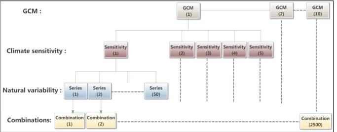
In this thesis, ten GCMs, five climate sensitivities and fifty series of natural variability were used to produce an array of climate change scenarios (i.e. 10×5×50=2500 climate scenarios). Four hydrological models were used to simulate future hydrological regimes of the Manicouagan River Basin, a northern watershed, based on these climate scenarios. Finally a probabilistic approach was used to conduct random samplings of the hydrological simulations produced by each individual hydrological model for the purpose of analyzing the uncertainty in selected hydrological variables. The main contribution of this study consists in the application of weighting schemes to evaluate various sources of uncertainty in the entire modeling process. In particular, the uncertainty due to climate sensitivity was explicitly investigated by assigning to it equal and unequal weights. No study to date has evaluated the major sources of uncertainty, from climate projections to hydrological modeling, by using weighting schemes. A few studies (e.g. Minville et al., 2008; Chen, 2011b) assessed various
sources of uncertainty on hydrological regimes, however they did not explore the effects of unequal weighting schemes on the hydrological response. In rare cases, studies estimated different sources of uncertainty through weighting experiments. However these were performed on a single hydrological variable such as, for example, low flows (e.g. Wilby and Harris, 2006). On the basis of existing researches, this thesis refines existing frameworks for evaluating the main sources of uncertainty in the simulated hydrological regimes of climate change studies. In particular, it makes innovative progress in evaluating the impacts due to GCM and climate sensitivity. The thesis also explores how assigning different weighting schemes to sources of uncertainty affects the return period of extreme hydrological events, which is a relevant aspect of the design of hydrological systems in the context of a changing climate.
CHAPITRE 2 LITERATURE REVIEW
This chapter provides general information about uncertainty and the empirical techniques and frameworks that appear in the scientific literature and that are used to evaluate the uncertainty in climate change impact assessments of watersheds hydrological response. First, the definition of uncertainty is discussed, with regard to the current understanding of natural world. Next, the major sources of uncertainty in climate change study are classified and briefly stated. General techniques used in recent research to estimate various sources of uncertainty in climate change projections and in the hydrological modeling process are also described. Finally, the advantages and limitations of the various approaches used are highlighted.
2.1 Definition of uncertainty
What is “uncertainty”? Why it always exists. How it propagates and how to reduce it.
Over the millennia, humans have struggled to increase their understanding and knowledge of the natural world. In doing so, they discovered ‘laws’ that helped them understand how things and events in the universe come into being. According to Dr. Sheldon Gottlieb (Gottlieb, 1997) “Science is an intellectual activity carried on by humans that is designed to discover information about the natural world in which humans live and to discover the ways in which this information can be organized into meaningful patterns. A primary aim of science is to collect facts (data). An ultimate purpose of science is to discern the order that exists between and amongst the various facts.”
Although science can quantitatively describe phenomena or forecast events, in a way that is very close to ‘reality’, the processes that are studied are more often than not incompletely known through a lack of understanding or information. This means that our representation of ‘reality’ is imperfect. Scientifically speaking, the gap between ‘reality’ and our description of
it is described as “uncertainty”. Uncertainty is often used to describe the state of being unsure, for example, in making some predictions of future events. Two published definitions of uncertainty are presented in this study:
a) A parameter associated with the result of a measurement that characterises the dispersion of the values that could reasonably be attributed to the measurand (ISO, 1993);
b) The lack of certainty, a state of having limited knowledge where it is impossible to exactly describe an existing state or a future outcome (Hubbard, 2010).
The first definition states the theoretical concept of uncertainty. The second is more relevant in explaining uncertainty in the context of climate change assessment studies.
The common and practical way of solving a wide range of biological, environmental and engineering problems is to build models (e.g. hydrological, transport/transformation, and biological models) to simulate natural processes. Uncertainty occurs and propagates in these models because of a number of factors, such as the randomness (variability) inherent to natural processes, errors due to imperfect human knowledge in developing the models, imprecise calibration of the parameters used to ‘fit’ the models to observations (Isukapalli, 1999), differences in temporal or spatial resolution between reality and simulation, and so on. The main sources of uncertainty in the modeling process are identified and classified in the next section.
Uncertainty exists therefore throughout the modelling process because the natural phenomena that are being represented are complex and the scientific knowledge is always incomplete. People must confront uncertainty, which is inevitable, in order to make better use of it.
Two general categories of uncertainty exist: random, or aleatory, and epistemic (Kiureghian and Ditlevsen, 2009). Aleatory uncertainty is used to describe the inherent variation
associated with the physical system or the environment under consideration (Oberkampf et al., 2004). Epistemic uncertainty, which is related to the human ability to understand and to describe nature, stems from a level of ignorance of the system or the environment. It is caused by a lack of knowledge or information in the modeling process. The common way to reduce epistemic uncertainty is to gather more data or to refine the models. Reducing aleatory uncertainty cannot be achieved as it is intrinsic to nature (Kiureghian and Ditlevsen, 2009).
2.2 Classification of uncertainty
Sources of uncertainty can be broadly classified as natural uncertainty, model uncertainty, parameter uncertainty and behavioral uncertainty (Isukapalli, 1999).
2.2.1 Natural uncertainty
It is a recognized fact that unavoidable unpredictability or “randomness” contributes to the inherently stochastic characteristic of natural systems and which is generally defined as natural uncertainty. Synonyms to natural uncertainty are aleatory uncertainty, random variability, stochastic uncertainty, objective uncertainty, inherent variability and basic randomness (Merz et al., 2005). If one admits that natural randomness exists, then observable phenomena cannot be precisely measured. But trends can be discovered via mean values. For example, according to the weather forecast, there will be rain tomorrow, but the exact time it will rain and the exact amount of rainfall cannot be forecasted, even though the ‘perfect’ model is available. Due to air movement, cloud formation, etc., it is virtually impossible to predict all information about a rainfall as such processes are random by nature. Broadly speaking though, natural uncertainty can be characterized by using ensemble averages, but the stochasticity inherent to natural processes makes the accurate estimation of system properties impossible (Isukapalli, 1999).
2.2.2 Model uncertainty
Mathematical models are commonly used to represent natural phenomena. However, the modeling process has inevitable consequences which are directly linked to the uncertainty in the choice of the model, known as “model uncertainty” (Cont, 2006). Model uncertainty is defined as the uncertainty of the model output and is related to the model’s inability to perfectly reproduce the dynamics of a natural system (Montanari, 2011). Model uncertainty may include mathematical errors, programming errors, statistical uncertainty (Farhangmehr and Tumer, 2009) and model structure uncertainty.
There are two types of mathematical errors: approximation errors and numerical errors. Approximation errors are errors due to approximate relationships used in models. Numerical errors stem from the selection of the computational method or technique (Thunnissen, 2003), for example, finite difference methods to solve differential equations. Other examples of mathematical errors in model results stem from the spatial or temporal resolution of the models. Programming errors refer to errors produced by computers and application programs (Hatton, 1997), such as bugs in hardware/software, errors in programming codes, inaccurate applied algorithms in simulation, etc. Statistical uncertainty arises from the process of extrapolating results of a statistical model, for example to generate extreme estimates (Bedford and Cooke, 2001). Finally, uncertainty in model structure is often acknowledged to be one of the principal sources of uncertainty (New and Hulme, 2000; Wilby and Harris, 2006; Christensen et al., 2010), arising from the incompleteness of a model and its inability to actually represent the difference between the real causal structure in the studied system and the perceived causal structure of the model. Therefore, choosing an inappropriate model in an ensemble of models to make simulations of interest may result in increased model uncertainty.
2.2.3 Parameter uncertainty
Parameter uncertainty has attracted researchers’ attention in recent literature (e.g., Wilby, 2005; Gitau and Chaubey, 2010; Jung et al, 2012). Parameter uncertainty is caused by the
lack of an adequate high quality database or by the inefficiency of the optimization algorithm used to obtain parameter values (Montanari, 2011). Generally speaking, parameter uncertainty stems from a set of parameters that is selected to run the mathematical model. Hydrological models incorporate many parameters that require sound estimations in order to produce reasonable results (Benke et al., 2008). However, due to the wide-range of applications and various degrees of complexity of hydrological models, it is not easy to quantify parameter uncertainty (Bergström et al., 2002; Blenkinsop and Fowler, 2007).
Hydrological model performance (and environmental models in general) is affected by parameter uncertainty (Wilby, 2005). In models, the true value of parameters is unknown because the data and the methods used to calibrate the models also have uncertainty. The usual way to quantify parameter uncertainty is to vary the parameter’s value and compare the model’s outputs (Benke et al., 2008). Probabilistic approaches, such as the Generalised Likelihood Uncertainty Estimation (GLUE) of Beven and Binley (1992) or the Markov Chain Monte Carlo (MCMC) of Hasting (1970), have been developed to address uncertainty, with respect to the specific aim of calibration and parameter estimation (Benke et al., 2008). However, it is not an easy task to identify a “true” set of parameters due to the parameterization equifinality, which is primarily caused by the dependence of the parameters (Beven, 2006). The concept of equifinality in hydrology suggests that different sets of parameters could result in same or similar predictions (Montanari, 2011). In other words, there is not a unique set of parameters for a hydrological modeling system, even with the same model structure, climate forcing and initial conditions (Tang and Zhuang, 2008). Thus, choosing an efficient optimization algorithm for estimating an “appropriate” set of parameters for the purpose of narrowing the range of parameter uncertainty becomes a crucial objective in the hydrologic community (Muttil and Jayawardena, 2008; Moradkhani and Sorooshian, 2009, Arsenault et al., 2013).
As more and more hydrological models were developed and applied in various studies, efforts were made to look for an effective optimization algorithm to calibrate hydrological models. For example, Singh et al., (2012) compared three different optimization algorithms,