Guay: CIRPÉE and CIREQ, Université du Québec à Montréal [email protected]
Guerre: Department of Economics, Queen Mary, University of London [email protected]
Lazarová: Department of Economics, Queen Mary, University of London [email protected]
The authors would like to thank Marcelo Fernandes, Liudas Giraitis, Bruce Hanse, George Kapetanios, Peter Phillips and Aris Spanos for stimulating questions or suggestions. They would also thank participants of the Queen Mary Econometric Reading Group, 2008 Oxbridge Time Series Workshop, 2008 Vienna Model Selection Workshop, 2008 North American Eocnometric Society Conference and 2008 European Econometric Society Conference, York Economic Seminar and Journées 2008 de Statistiques de Rennes. All remaining errors are ours. The first author gratefully acknowledges financial support of Fonds de recherche sur la société et la culture (FQRSC) and the Social Sciences and Humanities Research Council of Canada (SSHRC). The last two authors are thankful for the financial support from the Department of Economics of Queen Mary, University of London.
Cahier de recherche/Working Paper 09-25
Adaptive Rate-Optimal Detection of Small Autocorrelation Coefficients
Alain Guay
Emmanuel Guerre
Štěpána Lazarová
Abstract:
A new test is proposed for the null of absence of serial correlation. The test uses a
data-driven smoothing parameter. The resulting test statistic has a standard limit distribution
under the null. The smoothing parameter is calibrated to achieve rate-optimality against
several classes of alternatives. The test can detect alternatives with many small
correlation coefficients that can go to zero with an optimal adaptive rate which is faster
than the parametric rate. The adaptive rate-optimality against smooth alternatives of the
new test is established as well. The test can also detect ARMA and local Pitman
alternatives converging to the null with a rate close or equal to the parametric one. A
simulation experiment and an application to monthly financial square returns illustrate
the usefulness of the proposed approach.
Keywords: Absence of serial correlation, Data-driven nonparametric tests, Adaptive
rate-optimality, Small alternatives, Time series
1. Introduction
Testing for absence of correlation is important in many econometric contexts. Ignoring autocorrelation of the residuals in a linear regression model can lead to erroneous con…dence intervals or tests. Correlation of residuals from an ARMA model or of the square residuals from an ARCH model can indicate an improper choice of the order. In macroeconomics, dynamic stochastic general equilibrium models impose non correla-tion restriccorrela-tions as noted in Durlauf (1991). In …nance, the presence of autocorrelacorrela-tion can indicate a failure of an e¢ ciency condition or rational expectation hypothesis.
The earliest tests for absence of serial correlation were based on con…dence intervals for individual autocorrelation coe¢ cients as described in Brockwell and Davies (2006), Chat…eld (1989), Fan and Yao (2005) and Lütkepohl and Krätzig (2004). Tests of no correlation can be based on the percentage of sample autocorrelation coe¢ cients outside these individual con…dence bounds. A joint con…dence interval, based for instance on the null limit distribution of the maximal sample autocorrelation, can also be used. A second approach was established by Grenander and Rosenblatt (1952) and Bartlett (1954) who extended the goodness-of-…t tests such as Kolmogorov and Cramér-von Mises tests to testing for absence of serial correlation. Goodness-of-…t type tests for autocorrelation proposed by Durlauf (1991) and Anderson (1993) can detect Pitman local alternatives converging to the null with the parametric rate n 1=2, where n is the
sample size.
A third approach, initiated by Box and Pierce (1970), builds on a nonparametric method where a smoothing parameter needs to be selected. Hong (1996) has proposed a test for serial autocorrelation and Paparoditis (2000) has put forward a speci…cation test based on the spectral density function. These authors consider smooth alternatives in which the spectral density of the processes has bounded derivatives up to a given order. While Hong and Paparoditis have examined power of the test against …xed or local alternatives only, Ermakov (1994) has used a minimax approach to propose a test which is optimal in rate and in power against all alternatives of a given smoothness. The construction of the smoothed nonparametric tests of Ermakov (1994) and Hong (1996) uses the knowledge of the smoothness of the alternative, a characteristic which is generally not available to practitioners. This is a considerable limitation for practical applications of the smoothed nonparametric tests. As discussed in Section 4.1 below, existing plug-in bandwidth choices do not address this limitation in a satisfactory way.
The need to address the lack of knowledge of smoothness has spurred the development of adaptive methodology, leading to fully data-driven optimal tests. Fan (1996), Spokoiny (1996) and Horowitz and Spokoiny (2001) have studied adaptive tests based on some maximum statistics in the context of coe¢ cient model, continuous time white noise model and parametric regression speci…cation testing, respectively. Fan (1996) has noted that the asymptotic critical values of maximum tests do not perform well in practice and intensive bootstrap procedures must be used, see for example Horowitz and Spokoiny (2001). This contrasts with the simple data-driven smoothing parameter used by Guay and Guerre (2006) for dynamic model speci…cation testing based on a penalized test statistic. The test proposed by Guay and Guerre (2006) uses standard chi-square critical values and does not resort to simulation procedures that can be di¢ cult to implement in the time series context.
Adaptive methodology for serial correlation testing has been slower to develop. Fan and Yao (2005) outline, but do not analyze, an adaptive test for serial correlation which is based on the maximum of a set of Box-Pierce statistics. In our paper we set out to propose a data-driven test for absence of serial autocorrelation. In order to avoid pitfalls of the maximum tests mentioned above, we base the test on a penalized test statistic in the spirit of Guay and Guerre (2006). Our …rst contribution is to show that standard critical values such as chi-square or normal can be employed. This theoretical …nding is corroborated by a simulation study which shows that the level of the proposed test is close to its nominal size.
A second important contribution of the paper is to show that the knowledge of smoothness of the alternatives is not required and that the test is adaptive rate-optimal in the sense that it detects alternatives of unknown smoothness converging to the null at the fastest possible rate. We also consider a related class of ARMA-type alternatives with exponentially decreasing autocorrelation coe¢ cients where the rate of decrease is unknown, and demonstrate that the test is consistent against alternatives of this class which converge to the null with a rate close to n 1=2. The test can moreover detect Pitman local alternatives which converge
to the null with a rate close or equal to the parametric n 1=2.
A vast majority of the adaptive literature has been concerned with smooth alternatives. However, when looking at a plot of sample autocorrelation function, it is not easy for a practitioner to decide whether it is appropriate to describe the correlation function as smooth. A third contribution of the paper is therefore the introduction of a new class of alternatives that are not characterized by an abstract smoothness condition. On practical grounds, what matters when testing for no correlation is the proportion of large autocorrelation coe¢ cients. This consideration is at the core of the notion of sparse alternatives investigated by Ingster (1997) and Donoho and Jin (2004) in a Gaussian white noise model. A transposition of such alternatives to our context would induce us to introduce autocorrelation functions where among the …rst Pn lags, a number
Nn of autocorrelation coe¢ cients is equal to n or n for some given Pn, Nn and n. We develop a more
general class of alternatives where Nn is the number of autocorrelation coe¢ cients larger than n. In our
framework, the sequences Pn and n are not given a priori as in Ingster (1997) and Donoho and Jin (2004).
We propose a de…nition of adaptive rate-optimality of the test against a class that is described by a relation among Pn, n and Nn and develop a relevant theory to show that our test is adaptive rate-optimal against
this class of alternatives.
An interesting …nding is that alternatives with a high enough number of autocorrelation coe¢ cients larger than n can be detected by the new test even when n converges to zero at a rate faster than the parametric rate n 1=2. The ability to detect autocorrelations that converge to zero uniformly at a rate faster than n 1=2contrasts with many statistical frameworks and we refer to such fast-shrinking alternatives
as “small”. The paper gives an example of small alternatives that consist of high-order moving average processes with moving average coe¢ cients of order o n 1=2 . It is shown theoretically and through a simulation experiment that the Cramér-von Mises test has no power against such small moving average alternatives. This illustrates the potential bene…ts of using our data-driven nonparametric test. Examples of empirical time series where autocorrelation is detected by our test but not by the Cramér-von Mises test are considered in the application section.
The paper is organized as follows. Section 2 introduces the new adaptive test and states the assumptions. Section 3 states the main results which address the level of the new test, its consistency, adaptive rate-optimality against small and smooth alternatives as well as detection of ARMA-type and local Pitman alternatives. Section 4 reports the results of the simulation experiments and Section 5 applies the test to monthly squared …nancial returns. Section 6 summarizes the paper and mentions some potential applications of our methodology to other econometric testing problems. The proofs are gathered in two appendices.
2. Construction of the test and main assumptions 2.1. Construction of the test. Consider a parametric model
(2.1) m(Xt; Xt 1; : : : ; Xt p; ) = ut
and observations Xt, t = 1; :::; n. The scalar error term ut has zero mean and …nite variance and is
unob-servable when is unknown. We are interested in testing that ut is uncorrelated. For example, in AR(p)
model
Xt= 0+ 1Xt 1+ + pXt p+ ut;
correlated ut indicates a choice of too small order p. Another model of interest is the ARCH(p) model
(2.2) X 2 t 2 t 1 = ut; 2t = 0+ 1Xt 12 + + pXt p2 ;
where ut is uncorrelated if an appropriate order p is chosen. For many models, consistent estimators b
are available and ut can be estimated by residualsubt = ut(b). In some cases ut is directly observed. For
instance, in …nance, returns are directly observed, ut = Xt Xt 1, or observed up to a mean parameter,
ut= Xt Xt 1 where = E [Xt Xt 1] :
Suppose futg is a stationary process with zero mean and covariance function Rj = Cov(ut; ut+j). The
null and alternative hypotheses are
(2.3) H0: Rj = 0 for all j 6= 0; H1: Rj 6= 0 for some j 6= 0:
A natural estimator of the covariance is b Rj= 1 n nXjjj t=1 b utbut+jjj; j = 0; 1; : : : ; (n 1):
Let K be a kernel and p a smoothing parameter. Hong (1996) has based his test of no correlation on the test statistic (2.4) Sbp= n n 1 X j=1 K2 j p Rb 2 j:
Large values of bSp indicate evidence against the null. When K is the uniform kernel, K(t) = I(t 2 [0; 1]), bSp
is the Box-Pierce statistic
(2.5) BPdp= n p X j=1 b R2j:
Box and Pierce (1970) have shown that when the errors are independent and observed,ubt= ut, a normalized
statistic dBPp= bR20 is asymptotically chi-square distributed with p degrees of freedom, whereas for residuals
obtained from a well-speci…ed ARMA(s; q) model with independent innovations the limit distribution of d
BPp= bR02 is chi-square with degrees of freedom p s q. For uncorrelated but dependent and possibly
estimated futg, Francq, Roy and Zakoian (2005) show that the null limit distribution of dBPp= bR20is a mixture
of chi-square distributions. Romano and Thombs (1996) consider bootstrap procedures for uncorrelated but dependent futg.
When the kernel K is non-uniform, it is convenient to de…ne E(p) = n 1X j=1 1 j n K 2 j p and V 2(p) = 2 n 1X j=1 1 j n 2 K4 j p
which are approximations of the mean and variance of bSp= bR20 when errors ut are independent. The
no-correlation test of Hong (1996) is based on the studentized statistic
(2.6) Sbp= bR
2
0 E(p)
V (p) :
As shown by Hong (1996), the statistic (2.6) is asymptotically normal for ARMA models with independent identically distributed errors futg when p = pn diverges with the sample size. We note that for moderate
p, the quadratic nature of the statistic (2.6) suggests that chi-square or gamma approximation can be more accurate.
In practice, an important issue is the choice of an appropriate smoothing parameter p. We consider a data-driven smoothing parameterp that can take values in a set P. We assume that the set P is …nite andb has a dyadic structure
P = p; p 2; :::; p 2Q= p ;
where Q + 1 is the cardinality of P. Since p n 1, set P has at most O (ln n) elements. The structure of P is similar to the structure of the set of bandwidth values considered by Horowitz and Spokoiny (2001). The minimal value of the smoothing parameter, p = p
n, is chosen by the practitioner and can be bounded
or can grow with n.1 A test based on (2.6) for p = p would reject the null if bS
p= bR20 E(p) V (p)zn( ), where zn( ) satis…es (2.7) lim n!1P b Sp b R2 0 E(p) V (p)zn( ) ! = under H0.
The preceding two paragraphs suggest many correct choices of the critical value zn( ) under various kernels
K and parametric models generating the residualsubt.
Our aim is to …nd a data-driven smoothing parameter p such that the test based on bb Sp^ improves on
the test based on bSp in terms of power. Consider the following approximations of the mean and variance of 1A recommendation based on Theorems 4, 5 and 6 below would be to choose p as small as possible with p growing at most with the order ln n. In practice, choosing p = 1 may give simpler null limit distributions for uncorrelated but dependent futg. The test using p = 1 corresponds to the optimal likelihood ratio test of = 0for the Gaussian AR(1) model ut= ut 1+ "t.
( bSp Sbp)= bR20 when the errors ut are independent:
E(p; p) = E(p) E(p) and V2(p; p) = 2
n 1X j=1 1 j n 2 K2 j p K 2 j p 2 : We propose to selectp as the smallest maximizer of a penalized statistic,b
(2.8) p = arg maxb p2P b Sp b R2 0 E(p) nV (p; p) ! = arg max p2P b Sp Sbp b R2 0 E(p; p) nV (p; p) ! ;
where n > 0 is a penalty sequence which grows with n. The rationale behind such selection procedure is as follows. Under the null, the level of the test based on bSp is expected to be very close to its nominal
size. Hence the selection mechanism (2.8) is constructed in such a way that p is asymptotically equal to pb under the null. But using the …rst p correlation coe¢ cients may be insu¢ cient to detect some alternatives, in particular when p is small. Since ( bSp Sbp)= bR20 E(p; p) nV (p; p) = 0 when p = p, the expression on
the right of (2.8) shows thatp di¤ers from p when there is p 2 Pn p such thatb (2.9) ( bSp Sbp)= bR20 E(p; p) > nV (p; p):
Inequality (2.9) can be interpreted as statistical evidence that there are nonzero correlation coe¢ cients among lags p + 1; : : : ; p. Hence the test statistic bSp should be preferred to bSp for any value of p for which
inequality (2.9) is satis…ed. The procedure (2.8) selects the p 2 P for which the di¤erence between left- and right-hand sides in (2.9) is largest, ensuring that the test statistic will diverge under the alternative.
Under the null hypothesis of no correlation, the standardized values of bSp and bSp should not be
statis-tically di¤erent and the inequality (2.9) should not hold for any p provided n is large enough. It is then expected that bSbp = bSp, so that these two statistics should have asymptotically the same behavior. The
rejection region of the data-driven test is therefore
(2.10) Sbbp
b R2
0
E(p) V (p)zn( );
where the critical value zn( ) satis…es condition (2.7).2 The test (2.10) based on the optimized choice
p = ^p gains in power compared to the test based on the choice p = p. This can be seen from the following discussion. Suppose that K 0 is nonincreasing on [0; +1) so that E(p), V (p), E(p; p) and V (p; p) are increasing functions of p. De…nition (2.8) of ^p implies that
b Spb b R2 0 = max p2P b Sp b R2 0 E(p) nV (p; p) ! + E(bp) + nV (p; p)b b Sp b R2 0
E(p) nV (p; p) + E(bp) + nV (p; p)b for all p 2 P: Since E(p)b E(p) and V (p; p)b 0,
(2.11) Sbpb b R2 0 E(p) V (p)zn( ) b Sp b R2 0
E(p) nV (p; p) V (p)zn( ) for all p 2 P. 2An alternative studentization, Sb
b
p= bR20 E(bp) =V (p), would use the data-drivenb p.b However, simulation experi-ments of Guerre and Lavergne (2005) suggest that this studentization would give a test as powerful as the test using maxp2P Sbp= bR20 E(p) =V (p)proposed by Fan and Yao (2005) but less powerful than the test described by (2.10).
This gives the following lower bound for power of test (2.10): (2.12) P Sbpb b R2 0 E(p) V (p)zn( ) ! P Sbp b R2 0 E(p) V (p)zn( ) + nV (p; p) ! for all p 2 P. Since the penalization term nV (p; p) vanishes for p = p, it follows in particular that
(2.13) P Sbpb b R2 0 E(p) V (p)zn( ) ! P Sbp b R2 0 E(p) V (p)zn( ) ! :
Hence in terms of power, the test (2.10) improves on the test based on the statistic bSpwhich uses the smallest
smoothing parameter p. More generally, bound (2.12) indicates that up to a potential loss of power induced by the term nV (p; p), the test based on rejection region (2.10) is as powerful as the test based on the rejection region bSp= bR20 E(p) V (p)zn( ) for any p 2 P. This is an indication that the selection procedure
(2.8) is adaptive. Since the power bound (2.12) improves with decreasing n, the penalty term should be chosen as small as possible in order to maximize power.
2.2. Notation and main assumptions. In what follows, #A is the cardinality of the set A and C0; : : : ; C5
are positive constants. For two sequences fang and fbng, an bn means that fang and fbng have the same
order in the sense that there is a 0 < C < 1 such that janj =C jbnj C janj for all n. When studying the
performance of the test under the alternative, we consider a sequence fut;ng = fut;n; t 2 Ngn2Nof stationary
alternatives with autocovariance coe¢ cients fRj;n; j 2 Ngn2N. Our main assumptions are given below.
Assumption K. The kernel function K ( ) from R+ to (0; 1) is nonincreasing, bounded away from 0 on
[0; 1] and continuous over its compact support which is a subset of [0; 3=2].
Assumption P. Condition (2.7) holds. The penalty sequence n satis…es n> 0, n ! 1 and n= o (n) as n ! 1. The smoothing parameters set P is dyadic, P = p; 2 p; : : : ; 2Q p , with the largest element p = 2Qp and #P = Q + 1. The smallest element p may depend on n and p = o(p). For some s > 5=4 and
> 0, the maximal element p tends to in…nity and
(n= n)+2=(4s+1) p = o(n1=3) as n ! 1:
Assumption R. The sequence of alternatives fut;ng has zero mean, it is eighth order stationary with 1=C0
R0;n C0 and it has absolutely summable cumulants Cum ut1;n; : : : ; utq;n = n(t1; : : : ; tq) satisfying
+1
X
t2;:::;tq= 1
j n(0; t2; : : : ; tq)j C1Rq=20;n; q = 2; : : : ; 8:
Assumption M. The model (2.1), the estimator b and the sequence of alternatives fut;ng satisfy the
fol-lowing conditions:
(ii) The residuals ^ut= ut ^ admit a second order expansion
b
ut= ut;n+ (b n)0u(1)t;n+ kb nk2u(2)t;n
where fut;n; u(1)t;n; u (2)
t;ng is a stationary process with E1=2ku (1) t;nk2 C2, E1=2 u(2)t;n 2 C3 and 1 X j= 1 Ehut j;nu(k)t;n i C4; k = 1; 2; sup j2ZE 1 n n X t=1 ut j;nu(1)t;n E[ut j;nu(1)t;n] 2 C5 n :
Assumption K is weak. In particular, as is typical of the minimax approach adopted, for example, by Ingster (1993), it does not impose any conditions on the moments of the kernel. The compact sets [0; 1] and [0; 3=2] of Assumption K are somehow arbitrary and can be replaced by intervals [0; a] and [0; b] with 0 < a < b < 1. For a de…nition of cumulants in Assumption R, see for example Brillinger (2001, p. 19). In the Gaussian case, the cumulant summability condition is automatically satis…ed for q 3 since these cumulants are 0. When q = 2, the cumulant summability condition requires that
(2.14) 1 X j=1 Rj;n R0;n C1;
so that long range dependence is ruled out. A sequence of independent variables futg satis…es Assumption
R provided E [ut] = 0, Var (ut) = 2 > 0 and suptE u8t < 1. Assumption M(i) is standard and can
be veri…ed using regularity assumptions on the parametric model. Assumption M(ii) can be easily checked under suitable mixing conditions. Assumption M becomes vacuous if futg is directly observed.
3. Main results
An important issue in the construction of the test (2.10) is the choice of the penalty sequence. The discussion of the construction of the test in Section 2 has revealed that choosing nlarge enough guarantees that under the null, the distribution of the test statistic Sbbp= bR20 E(p) =V (p) is standard and chi-square
or normal critical values can be employed. On the other hand, power considerations based on bound (2.12) lead to a small n penalty recommendation. The trade-o¤ of the size and power concerns is analyzed in
Sections 3.1, 3.3 and 3.4. It transpires in Section 3.1 that the lower bound for penalty n for which a test of the desired level is obtained is of rate (2 ln ln n)1=2. It is then shown in Sections 3.3 and 3.4 that this rate is low enough to ensure that our test is adaptive rate-optimal under both small and smooth alternatives. Section 3.2 gives a general consistency result that holds under weaker conditions than the rate-consistency results. Sections 3.5 and 3.6 examine the performance of the test against ARMA-type and Pitman local alternatives.
3.1. Asymptotic level of the test. The following theorem gives a lower bound for n which ensures that the test is asymptotically of level under independence.
Theorem 1. Let Assumptions K and P hold. Assume that futg is independently distributed and satis…es
Assumptions M and R. If the penalty sequence f n; n 1g satis…es
(3.1) n (2 ln ln n)1=2+ for some > 0; then
lim
n!1P bp = p = 1
and the test (2.10) is asymptotically of level .
The discussion following Proposition 1 in Section 3.3 shows that choosing n = o (2 ln ln n)1=2 gives a test with a degenerate asymptotic level equal to one and therefore that one cannot improve on (3.1) in terms of rate. A conjecture is that the order (2 ln ln n)1=2 cannot be improved in constant either. A heuristic argument is as follows. Since E(p; p) = 0 and V (p; p) = 0, the de…nition (2.8) ofp givesb
(3.2) P bp 6= p = P max p2Pnfpg ( bSp Sbp)= bR20 E(p; p) V (p; p) ! n ! :
To simplify the discussion, assume that the kernel is uniform so that bSp is the Box-Pierce statistic (2.5) and
b
Sp Sbp = nPpj=p+1Rbj2. For 1 j p, variables n bRj2= bR20 are asymptotically independent and identically
distributed and nSbp Sbp; p 2 P
o
behaves asymptotically like a partial sum process. Since p = p2q for
q = 1; :::; Q and V2(p; p) = 2p (1 + o(1)) for large p, a candidate Gaussian approximation of the statistics in
(3.2) is (3.3) ( ( bSp Sbp)= bR20 E(p; p) V (p; p) ; p 2 P n fpg ) d ' ( W p2q p1=22q=2; q = 1; :::; Q ) d = W (2 q) 2q=2 ; q = 1; :::; Q ;
where W is a Brownian motion process on [0; 1). The discrete-time Gaussian Markov process W (2q)=2q=2
is a stationary AR(1) process with autoregression coe¢ cient 1=21=2 because
Cov 0 @W (2q) 2q=2 ; W 2q0 2q0=2 1 A = 2 jq2q0j:
Hence, since Q ln n, it follows from a theorem of Berman (1962, p. 96) that
(3.4) max q=1;:::;Q W (2q) 2q=2 = (2 ln Q) 1=2 + oP(1) = (2 ln ln n)1=2+ oP(1):
Therefore (3.1) implies that limn!1P bp = p = 1. The bound (3.4) together with (3.2) and (3.3) suggest
that limn!1P p = p = 0 ifb n ((2 ) ln ln n) 1=2
for some in (0; 2). Hence limn!1P p = p = 1b
should imply n (2 ln ln n) 1=2
. The order (3.4) also shows that the bound (3.5) n (2 ln Q)1=2+ for some > 0; may work better than (3.1) in small samples.
3.2. Consistency. In this section we give a general consistency result for alternatives with a maximal correlation coe¢ cient bounded away from zero. The subsequent sections then examine rate consistency and adaptive rate-optimality against several speci…c classes of alternatives.
Theorem 2. Let Assumptions K and P hold. Assume that n= O(p1=2). Consider a sequence of alternatives
fut;ng satisfying Assumption M with
1=C R0;n= O(1); 2n X j=1 R2 j;n R2 0;n = o(n) and with fourth order cumulant n satisfying
1
X
t2;t3;t4=1
j n(0; t2; t3; t4)j = O(1)
Then if max1 j pjRj;n=R0;nj > 0, the test is consistent.
Theorem 2 does not employ Assumption R and admits processes with long range dependence, including fractional Gaussian processesn(1 L) d"t
o
of order d < 1=2.
When testing for no autocorrelation, there are alternatives against which no test is consistent. Consider a sequence of moving average processes
(3.6) ut;n = "t "t n; 6= 0,
where "tis independent identically distributed with mean zero and variance 2. The sample fu1;n; :::; un;ng
consists of independent variables and no test will detect correlation. In the terminology of Ingster (1993), H0
and H1 in (2.3) are indistinguishable or, according to Pötscher (2002), testing H0 against H1is an ill-posed
problem. Condition max1 j pjRj;n=R0;nj > 0 of Theorem 2 precludes ill-posed problems by limiting
the set of admissible alternatives. However, this condition is not overly restrictive. Since p tends to in…nity, Theorem 2 shows that our test is consistent against sequence of alternatives in a growing set H1;n( ) which
asymptotically contains all the alternatives such that maxj 1jRj=R0j > 0.
3.3. Small alternatives. Under stronger assumptions, it is possible to improve on Theorem 2 and to consider alternatives converging to the null such that maxj 1jRj;n=R0;nj n for some n! 0. Given such
a choice of n, correlation coe¢ cients larger than n can be viewed as large. As discussed in Section 3.2
and in the introduction, alternatives that can be detected must have enough large correlation coe¢ cients at small enough lags, say j Pn. To quantify the number of large correlation coe¢ cients, we de…ne
(3.7) Nn= Nn(fut;ng ; Pn; n) = # fjRj;n=R0;nj n; 1 j Png :
Correlation coe¢ cients smaller than ncan be seen as negligible and the proportion Nn=Pncan be interpreted
as an indicator of sparsity. The following theorem states a condition on Pn and n which guarantees
consistency of the test. The condition requires that there exist a suitable pair (Pn; n) satisfying a sparsity
restriction. The testing procedure in‡uences the smallest possible rate ncompatible with detection through the penalty sequence n and a constant that depends on the kernel K and the set P.
Theorem 3. Let Assumptions K and P hold. Consider a sequence of alternatives fut;ng satisfying
Assump-tions M and R. The test (2.10) is consistent against the sequence of alternatives fut;ng if there exists some n> 0 and Pn2 [p; p] such that for n large enough,
(3.8) n n1=2 nP 1=2 n Nn !1=2 ; where does not depend on the alternative fut;ng.
The consistency condition (3.8) allows for alternatives where n and Pn can be chosen such that
(3.9) n 1 n1=2 nP 1=2 n Nn !1=2 :
Of special interest is the case where limn!1 nP 1=2
n =Nn= 0 since (3.9) shows that the test can detect small
alternatives, that is alternatives with correlation coe¢ cients converging to the null at a rate that is faster than the parametric rate n 1=2. The condition lim
n!1 nP 1=2
n =Nn= 0 requires that the number Nnof large
correlation coe¢ cients jRj;n=R0;nj, 1 j Pn, diverges faster than nP 1=2
n . This allows for “saturated”
alternatives with Nn = Pn and limn!1Pn1=2= n = 1 but also for sparse alternatives with Nn=Pn = o (1)
provided that the sparsity indicator Nn=Pndoes not go to 0 too fast, satisfying limn!1(Nn=Pn)(Pn1=2= n) =
1.3
Let us now investigate the adaptive optimality of the rate n in (3.8). Observe that the smaller the
the better the consistency rate. Though for our test procedure the is …xed once the kernel and the set P are chosen, one might ask whether there exist better tests that would detect alternatives satisfying a bound like (3.8) but with a which converges to zero when the sample size increases. The following proposition gives a negative answer to this question when n has the smallest possible order (2 ln ln n)1=2for which the test is asymptotically of level .
Proposition 1. Let the process futg be observed and suppose Assumption P holds. Then for any 0 <
< 1 there exists a sequence of alternatives fut;ng satisfying Assumption R that cannot be detected by any
asymptotically -level test, 2 (0; 1), although there is a Pn 2 p; p and a n ! 0 so that
n 1 n1=2 (2 ln ln n)1=2Pn1=2 Nn(fut;ng ; Pn; n) !1=2 ; lim n!1 Nn(fut;ng ; Pn; n) (2 ln ln n)1=2Pn1=2 = 1: .
Proposition 1 implies that when n is asymptotically proportional to (2 ln ln n)1=2, our test is adaptive rate-optimal. Indeed, by Theorem 3, our test is consistent against the alternatives for which
(3.10) n n 1=2(2 ln ln n)1=4Pn1=4Nn1=2
3This contrasts with Ingster (1997) and Donoho and Jin (2004) who only achieve the consistency rate (ln n=n)1=2 for very sparse alternatives where Nn=Pn goes to 0 with a faster rate. On the other hand, although their results are obtained in a nonadaptive simple setup, it suggests that our test is not optimal against such very sparse alternatives.
under the assumptions of Proposition 1. However, neither our test nor any other will detect alternatives for which n (1 ) n 1=2(2 ln ln n)
1=4
Pn1=4Nn1=2where 2 (0; 1). This means that when n (2 ln ln n) 1=2
, the in (3.10) cannot approach zero, hence the adaptive rate-optimality.
Proposition 1 further implies that there are alternatives satisfying
n 1 n1=2 0 @o (2 ln ln n) 1=2 Pn1=2 Nn 1 A 1=2
that cannot be detected by any nondegenerate asymptotic -level tests. Hence tests that can detect such alternatives are asymptotically trivial and must always reject the null. Since Theorem 3 shows that choosing
n= o (2 ln ln n) 1=2
would permit detection of these alternatives, the resulting test must have a degenerate asymptotic level equal to one, implying that the rate (2 ln ln n)1=2 in the bound (3.1) of Theorem 1 cannot be improved.
As an example of small alternatives that satisfy (3.9), consider the following sequence of high-order moving average processes,
(3.11) ut;n= "t+ 1=2 n n1=2P1=4 n Pn X k=1 k"t k; lim n!1Pn = 1;
where f"tg is a white noise with variance 2 and is a scaling constant. The following lemma describes the
covariance function of fut;ng in (3.11).
Lemma 1. If PPn
k=1 2
k = O(Pn), Pn = o((n= n)2=3) and limn!1 nn 1 = 0, then alternatives (3.11)
satisfy R0;n= 2 1 + O nPn1=2=n and, uniformly in 1 j Pn, Rj;n= 1=2 n n1=2P1=4 n j 2+ o 1=2 n n1=2P1=4 n ! :
A distinctive feature of alternatives (3.11) when max1 k Pnj kj = O (1) is that both their moving average
and correlation coe¢ cients approach zero uniformly faster than n 1=2 provided P
n= 2n tends to in…nity. Let
us now check consistency of the test under the assumption that mink2[1;Pn] k
2 1. Our choice of n is (3.12) n= 2 1=2 n n1=2P1=4 n :
Lemma 1 states that the number of large correlations is asymptotically equal to Pn, that is Nn = Pn(1 + o(1)).4
The choice of n in (3.12) is such that
n= 2n1=2 nP 1=2 n Nn !1=2 (1 + o (1)) ; 4Condition N
n= Pn(1 + o(1))implies that the alternatives (3.11) are saturated, that is, there are no kcoe¢ cients equal to zero . Introducing more sparsity, that is setting some coe¢ cients to zero, would not a¤ect Proposition 2 below provided limn!1 (ln ln n)1=2Pn1=2=Nn = 1. Corresponding alternatives (3.11) would have only Nn nonzero kcoe¤…cients and a normalization factor 1=2n Pn1=4=(nNn)1=2instead of 1=2n =(n1=2Pn1=4).
so that (3.8) holds provided 2 and Theorem 3 shows that the test is consistent if p Pn p.
Consistency of our test against alternatives (3.11) contrasts with the performance of other testing procedures. Due to the small o n 1=2 order of the moving average and correlation coe¢ cients, standard
con…dence interval procedures will fail to detect serial correlation. The next proposition implies that the Cramér-von Mises (CvM) test of Durlauf (1991) is also not consistent against the alternatives satisfying (3.11). The CvM test is based on the following statistic:
(3.13) CvM = n2 n 1X j=1 b R2 j j2Rb2 0 :
Proposition 2. Let futg be observed. Consider alternative (3.11) with independent Gaussian "twith mean
zero and variance 2. Assume PPn
k=1 2
k = O(Pn), max1 k Pnj kj = O (1) ; min1 k Pn k 2 1 and
> 0. Assume that n! 1 with, for some C > 0 and > 0 small enough, n C ln n and 1=2+n =C Pn C n 2 nln n 2=3 :
Then the test statistic (3.13) has the same limit distribution under the alternative and under the null of independence, and the CvM test is not consistent.
The small alternatives considered here also illustrate the di¤erence between rates for estimation and testing. While the best possible rate for estimation of the moving average or correlation coe¢ cients is the parametric rate n 1=2, our test can detect coe¢ cients that tends to zero at a faster rate than the parametric rate.
3.4. Smooth alternatives. This section considers alternatives with a smooth spectral density. For an integer number s, let eC(L; s) be the class of zero-mean stationary processes whose normalized spectral density function f0( ) has sth derivative f0(s)( ) with mean-square norm smaller than 1=2L. Since
f0(s)( ) = 1 2 +1 X j= 1 Rj R0
(ij)sexp(ij ) and
Z f0(s)( )2d = 1 +1 X j=1 j2s Rj R0 2 ; this class of functions can be de…ned also for noninteger s using the summability conditionP+j=11j2s(R
j=R0)2
L2. Restricting the class eC(L; s) to processes utsatisfying Assumption R, we de…ne
C(L; s) = 8 <
:futg: futg satis…es Assumption R and
1 X j=1 j2s Rj R0 2 L2 9 = ;; L; s > 0:
Much attention has been paid to hypothesis testing when the number of derivatives s is known, see for example work of Hong (1996), Paparoditis (2000) and the references therein. We focus here on the case where the smoothness indexes L and s of the alternatives are unknown and can depend on the sample size. In this context, Spokoiny (1996) has shown that when usingP1j=1(Rj=R0)2 as a measure of the deviation
from the null, the optimal adaptive consistency rate is5 (3.14) Rn(L; s) = L1=(4s+1)
(ln ln n)1=2
n
2s=(4s+1)
.
5Spokoiny (1996) considers the ideal continuous-time white noise model. The equivalence result of Golubev, Nussbaum and Zhou (2009) shows that this rate is also adaptive optimal for directly observed Gaussian futg with s > 1=2. This is su¢ cient to show that the adaptive optimality statement of Spokoiny (1996) extends to the case where the process futg is directly observed.
The following theorem shows that the test is adaptive rate-optimal when n (2 ln ln n)1=2.
Theorem 4. Let Assumptions K and P hold with p = O (lnan), a > 0. Assume that n is of order (ln ln n)1=2. Let L
n and sn be two sequences of positive real numbers such that for s as in Assumption P,
and for C large enough,
(3.15) s sn = o(ln n); and Cp sn+14 n 23=2s nn 1=2 Ln p C sn+14 n 23=2s nn 1=2 : Let fut;ng be a sequence of alternatives in C(Ln; sn) satisfying Assumption M.
The test (2.10) is consistent if, for > 0 large enough,
1 X j=1 Rj;n R0;n 2 2 R2n(Ln; sn);
where does not depend on Ln and sn or on the alternative fut;ng.
The main bene…t of smoothness adaptation is as follows. Tests that are designed for a speci…c class C (L1; s1)
are in general suboptimal for smoother alternatives in C (L2; s2) with s2> s1. In contrast, our test achieves
the best adaptive optimal detection rates over the two classes of alternatives, achieving in particular a better rate for the smoother alternatives.
Theorem 4 does not require Ln to be bounded away from zero and sn to be bounded from above. This
extends existing adaptive results.6 Consider for instance Pitman local alternatives converging to the null at
the rate Ln! 0,
(3.16) ut;n= "t+ Lnvt,
where f"tg is a strong white noise and where E [vt] = 0, Var("t) = Var(vt) = 1, Cov ("t j; vt) = rj for j > 0
and 0 for j 0 withP1j=1j2sr2j < 1 for s s, and f"t; vtg is a stationary process with Cov (vt; vt j) = cj.
The covariance function of the process fut;ng in (3.16) is given by
(3.17) R0;n= 1 + L2n; Rj;n= Lnrj+ L2ncj:
If fvtg is in C(1; s) then fut;ng is in C(L0n; s) with L0n = O(Ln) because P1j=1j2sr2j < 1. If p = O (1),
(3.15) holds for a smoothness parameter Ln converging to zero at the rate of (ln ln n)1=4=n1=2. In this case, 1 X j=1 Rj;n R0;n 2 = (1 + o(1)) L2n 1 X j=1 rj2 (ln ln n) 1=2 n 1 X j=1 r2j: Since R2n(L0n; s) (ln ln n)1=2 n ! 1 4s+1 (ln ln n)1=2 n ! 4s 4s+1 =(ln ln n) 1=2 n ;
Theorem 4 shows that the test (2.10) is consistent against Pitman local alternative (3.16) providedP1j=1r2 j is
large enough. Hence the test can detect Pitman alternatives converging to the null at the rate of Rn(L0n; s)
(ln ln n)1=4=n1=2. This rate improves on the rates derived by Hong (1996) and Paparoditis (2000). 6Spokoiny (1996), Fan (1996), Horowitz and Spokoiny (2001) and Guerre and Lavergne (2005) do not allow for s
n ! 1, Ln! 1 or Ln ! 0: The inequality (3.15) allows for Ln (n= n)
1=2+,
2 (0; 1=2). If p = O(1), then (3.15) allows for Ln (n= n)
3.5. Pitman alternatives. The detection rate (ln ln n)1=4=n1=2derived for local alternatives (3.17) can be improved upon when correlation coe¢ cients with j p are large enough. The best rate for Pitman local alternatives allowing for consistency is 1=o n1=2 which is the best consistency rate for the optimal
Neyman-Pearson test that compares the likelihood of the null hypothesis and of the local alternative. Theorem 5 implies that the test can achieve the rate 1=o n1=2 for some Pitman alternatives provided p = O(1). The
following theorem admits long range dependence processes but restricts the memory parameter to d < 1=4. Theorem 5. Let Assumptions K and P hold. Consider a sequence of alternatives satisfying Assumption M and 1=C R0;n C, 1 X j=0 Rj;n R0;n 2 = O(1) and +1 X j2;j3;j4= 1 j n(0; j2; j3; j4)j = O(1): Then if (n=p)1=2max
1 j pjRj;n=R0;nj ! 1, the test (2.10) is consistent.
3.6. ARMA-type alternatives. A class of alternatives of practical interest consists of ARMA-type al-ternatives whose correlation function decreases at an exponential rate. The following theorem addresses detection of alternatives with a correlation function going to zero at an unknown exponential rate. The detection rate achieved by our test is very close to the parametric rate.
Theorem 6. Let Assumptions K and P hold. Let p = o(ln n), n ! 1 and n = o(p1=2). Consider a sequence of alternatives fut;ng satisfying Assumptions M and R and such that, for some unknown r 2 (0; 1)
and L > 0, Rj;n R0;n L 1 r 2 2 ln (1=r) 1=2 rj for all j 1. Then the test (2.10) is consistent if, for > 0 large enough,
1 X j=1 Rj;n R0;n 2 2(1 + o(1)) n n 0 @ln (Lr) 2 n= n ln(1=r) 1 A 1=2 ;
where does not depend on L and r or on the alternative fut;ng.
Choosing a penalty sequence n of order (ln ln n)1=2 that satis…es (3.1) leads to a test of asymptotic level with a tractable null distribution. The consistency rate of such test is (ln ln n)1=4(ln n)1=4=n1=2. Inspection
of the proof of the theorem reveals that if we chose instead a penalty p = (2 ln ln p)1=2(1 + "), we would obtain a test with a slightly better consistency rate of (ln ln ln n)1=4(ln n)1=4=n1=2. However this test would
have a nonstandard null limit distribution and may be di¢ cult to use in practice.
4. Simulation experiments
In this section, we investigate small sample properties of the test (2.10), hereafter GGL. We compare the performance of our test with the performance of a data-driven test procedure based on an integrated mean square error (IMSE) criterion (hereafter M test) and of the Cramér-von Mises (CvM) test (3.13).
Two versions of the test (2.10) are considered. The …rst version uses the uniform kernel for which the test statistics ^Sp in (2.4) becomes the Box-Pierce statistics (2.5). The second version uses the Parzen kernel
(4.1) K(x) = 8 > > < > > : 1 6x2+ 6jxj3; jxj 1=2; 2(1 jxj)3; 1=2 < jxj 1; 0 otherwise.
4.1. Benchmark tests. The critical values of the CvM are given in Anderson and Darling (1952). The simulation experiments of Durlauf (1991) show that these critical values give a level close to the nominal level for sample sizes as small as n = 50. To construct the M test, we follow Hong (1999) and Hong and Lee (2005) in considering a test statistic
(4.2) M = M (pbIM SE) =
SpbIM SE E (pbIM SE)
V (pbIM SE)
;
wherepbIM SE is data-driven and where the Parzen kernel (4.1) is used in the de…nition of ^Sp.7 The M test
rejects absence of correlation if M zn( ) where zn( ) is a critical value usually given by the normal
distribution, see Hong (1996, 1999). To de…nepbIM SE, observe …rst that
b Sp= n 2 b R2 0 Z ^ fn( ; p) 2 d ; f^n( ; p) = 1 2 1 X j= 1 K j p Rbjexp ( ij ) .
In the formula above, ^fn( ; p) is a nonparametric kernel estimator of the spectral density function f ( ) =
P1
j= 1Rjexp ( ij ) =(2 ). Following a proposal of Andrews (1991) and Newey and West (1994), Hong
(1999) and Hong and Lee (2005) used a data-driven parameter p that asymptotically achieves the minimum of the integrated mean squared error of ^fn( ; p) de…ned as
(4.3) IM SE( ^fn( ; p); f ) = E
Z
j ^fn( ; p) f ( )j2d :
For the Parzen kernel (4.1) and twice di¤erentiable spectral density, the ideal smoothing parameter pIM SE=
arg min IM SE( ^fn(p); f ) is asymptotically of order n1=5, pIM SE = cn1=5(1 + o (1)). Robinson (1991a) has
shown that lim n!1n 4=5IM SE( ^f n( ; p); f ) = Z jf( )j2d c Z K2(x) dx + Z jf(2)( )j2d K (2)(0) 2c2 2 ; therefore the optimal constant c in the expansion pIM SE = cn1=5(1 + o (1)) is equal to
c (f ) = K (2)(0)2 R jf(2)( )j2d R K2(x) dx R jf( )j2d !1=5 = 144 P1 j= 1j4R2j 0:539285P1j= 1R2 j !1=5 : The data-driven smoothing parameterbpIM SE in (4.2) is based on an estimated value of c (f ),
(4.4) pbIM SE =bc1=5(f ) n1=5, where bc(f) =
144Pn 1j= (n 1)K (j=p) je 4Rb2j 0:539285Pn 1j= (n 1)K (j=p) be R2
j
; andp is a pilot bandwidth set toe p = (4n=100)e 4=25as in Newey and West (1994).
A …rst di¢ culty with the data-driven pbIM SE concerns the null limit distribution of the test statistic
M . Hong (1999) and Hong and Lee (2005) have shown that M = M (pbIM SE) behaves asymptotically as
M (pIM SE) provided that c (f ) > 0 and bc(f) =c (f) tends to 1 in probability at a su¢ ciently fast rate.
Unfortunately, such a result is mostly useful under the alternative since c(f ) = 0 under the null, so that this result cannot be used to derive the null limit distribution of M (pbIM SE). The common practice is to
ignore this issue and to regard the random pbIM SE as deterministic when computing the critical values of
M (pbIM SE). This contrasts with our method of choosing the data-driven ^p since in our case the test statistics
has a clear-cut null limit distribution.
A second issue with the data-driven pbIM SE concerns its behavior under the alternative. Alternatives
converging to the null may give a c (f ) which is close to zero or tends to zero, so that the aforementioned result of Hong (1999) and Hong and Lee (2005) may not apply. More importantly, the data-driven pbIM SE
is derived from the minimization of the criterion (4.3), which is designed for estimation of spectral density functions and may not be appropriate for testing. For instance, it follows from the results of Ermakov (1994) that the nonadaptive optimal bandwidth for testing against alternatives with twice di¤erentiable spectral density is n2=9which is slightly larger that the order n1=5used in (4.4). Furthermore, the fact that the data-drivenpbIM SE is calibrated for twice di¤erentiable spectral density functions limits the adaptive properties
of the M test.
4.2. Other details of the simulation experiments. We consider experiments with 10; 000 replications of samples of size n = 200 and 1; 000. As suggested in (3.5), we use a penalty sequence n which depends on the cardinality Q + 1 of the set P of admissible smoothing parameters. Some preliminary experiments have shown that
n= (2 ln Q)1=2+ 3:2
works well. For the case with 200 observations, we use P = f2; 4; 8; 16; 32g. With 1,000 observations, p is also set to 2 but P increases to f2; 4; 8; 16; 32; 64; 128; 256g. The rejection region (2.10) makes use of critical values
(4.5) zn( ) = zn ; p =
cn ; p E p
V p
where the choice of cn( ; p) depends on the kernel. The rejection region (2.10) and (4.5) implies that the
test rejects if bSpb cn( ; p) bR20. In the case of uniform kernel, cn( ; p) is given by the chi-square distribution
with p degrees of freedom. For the Parzen kernel, cn( ; p) is given by a gamma distribution ( ; ) with
shape and scale parameters that match the null approximations of the mean and variance of ^Sp,8
= E p
2
V2 p and =
E p V2 p .
The M test uses the gamma critical values zn( ;pbIM SE).
8The theoretical justi…cation of our gamma approximation is given by Shorack (2000), Theorem 4.1. Note also that for the uniform kernel, E p = pand V2 p = 2pasymptotically and ( ; )is equal to a chi square with p degrees of freedom. Observe also that limp!1zn( ; p)is the 1 quantile of the standard normal distribution.
4.3. Under the null. We consider independent sequences distributed respectively as a standard normal, a Student with 5 degrees of freedom and a centered and standardized chi-square with 1 degree of freedom. The experiments with the Student distribution allow us to examine the behavior of the testing procedures when heavy tail processes are present whereas the chi-square distribution allows us to examine the sensitivity to skewness. The chi-square distribution also arises when investigating ARCH speci…cations (2.2) with Gaussian error terms.
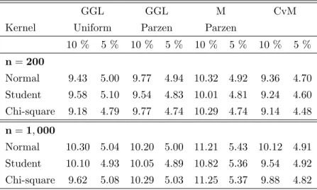
Table 1 reports the associated rejection rates. For the experiments with 200 observations, the empirical levels for all testing procedures are close to the nominal levels. Under the null, the choice of the kernel does not seem to a¤ect the rejection rate of our procedure. Those results are not very sensitive to the choice of distribution for the white noise. For the experiments with 1,000 observations, the empirical levels are very close to the nominal levels for all testing procedures and all distributions with the exception of the M test, which slightly overrejects for all cases.
GGL GGL M CvM
Kernel Uniform Parzen Parzen
10 % 5 % 10 % 5 % 10 % 5 % 10 % 5 % n= 200 Normal 9.43 5.00 9.77 4.94 10.32 4.92 9.36 4.70 Student 9.58 5.10 9.54 4.83 10.01 4.81 9.24 4.60 Chi-square 9.18 4.79 9.77 4.74 10.29 4.74 9.14 4.48 n= 1; 000 Normal 10.30 5.04 10.20 5.00 11.21 5.43 10.12 4.91 Student 10.10 4.93 10.05 4.89 10.82 5.36 9.54 4.92 Chi-square 9.62 5.08 10.29 5.03 11.25 5.37 9.88 4.82
Table 1: Level of tests.
4.4. First set of alternatives: Cramér-von Mises alternatives. We consider autoregressive and moving average alternatives
(4.6) AR(P; ) : ut= ut P + "t and M A(P; ) : ut= "t+ "t P:
In the simulation, the noise f"tg is a sequence of i.i.d. standard normal variables. The MA(P; ) alternatives
are similar to the moving average processes de…ned in (3.6) but with moderate values of P = 1; 4 or 6. De…ne the Cramér-von Mises distance DCvM as a theoretical counterpart of 2CvM=n in (3.13);
DCvM2 = n 1X j=1 R2 j j2R2 0 :
The values of parameters and in (4.6) solve (4.7) n 2D 2 CvM(AR(P; )) = 3 2 and n2DCvM2 (M A(P; ))) = 32;
respectively, for n = 200 and 1; 000 and for P = 1; 4 or 6. Solutions of (4.7) are given in Table 2 below. The numerical value 3 in (4.7) has been chosen because 3= 2' 0:3040 which is close to the 90% quantile of the
CvM null limit distribution. Elementary algebra gives D2CvM(AR(P; )) = 1 X k=1 2k (P k)2 = D2 CvM(AR(1; )) P2 and D 2 CvM(M A(P; )) = 2 P2(1 + 2)2:
Hence the solutions of (4.7) are such that (4.8) P;n=3
1=2P
n1=2 (1 + o (1)) and P;n=
31=2P
n1=2 (1 + o (1)) ;
and the processes de…ned in (4.6) can be seen as n1=2 local Pitman alternatives up to a negligible term.
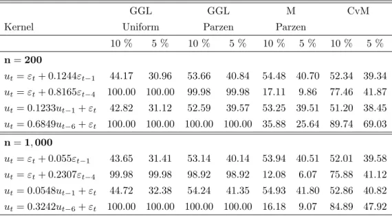
Simulation results are summarized in Table 2.
For AR(1) and MA(1) processes, the procedure GGL with Parzen kernel performs similarly to the M test and the CvM test while the GGL procedure with uniform kernel is less powerful. The underperformance of the GGL test when the kernel is uniform can be due to shape of the kernel and the choice of p. Since p= 2 in the simulation experiments, the uniform kernel puts the same weight on the …rst and second order autocorrelation although the …rst order autocorrelation is more important for these alternatives, particularly for the MA(1) process. The additional weight on the second order autocorrelation coe¢ cient increases the variance of the test statistic but is not helpful for detection of M A(1) alternatives. In contrast, the fact that the Parzen kernel and the CvM test correctly put more weight on the …rst order autocorrelation coe¢ cient explains why they perform better.
With increasing P , the power of the CvM test increases9. However, for processes with a higher order P
(MA(4) and AR(6)), our procedure has a power close to one and substantially outperforms the CvM test. This is due to the fact that increasing P increases the size of the maximal correlation coe¢ cients, as can be seen from (4.8), and to the fact that our test is more sensitive to high order correlations than the CvM test. The M test performs poorly against the higher order alternatives (4.8). This is because the data-driven b
pIM SE is too small in a vast majority of the simulations.
4.5. Second set of alternatives: small correlation coe¢ cients. This section considers alternatives (3.11). More speci…cally, we consider
(4.9) ut= ut(P; b) = "t+ (3 n) 1=2 n1=2P1=4 P X k=1 k;b"t k, k;b i.i.d. N (0; 1) .
9This can be explained by the fact that E 2CvM = D
CvM+ nP1j=1Var Rbj =j2. Further inspection of our simulation experiments shows that E 2CvM can be up to twice larger than 3 = D
CvM, hence the important impact of the term nP1j=1Var Rbj =j2.
GGL GGL M CvM Kernel Uniform Parzen Parzen
10 % 5 % 10 % 5 % 10 % 5 % 10 % 5 % n= 200 ut= "t+ 0:1244"t 1 44.17 30.96 53.66 40.84 54.48 40.70 52.34 39.34 ut= "t+ 0:8165"t 4 100.00 100.00 99.98 99.98 17.11 9.86 77.46 41.87 ut= 0:1233ut 1+ "t 42.82 31.12 52.59 39.57 53.25 39.51 51.20 38.45 ut= 0:6849ut 6+ "t 100.00 100.00 100.00 100.00 35.88 25.64 89.74 69.03 n= 1; 000 ut= "t+ 0:055"t 1 43.65 31.41 53.14 40.14 53.94 40.51 52.01 39.58 ut= "t+ 0:2307"t 4 99.98 99.98 98.92 98.92 12.08 6.07 75.88 41.12 ut= 0:0548ut 1+ "t 44.72 32.38 54.24 41.35 54.93 41.80 52.86 40.82 ut= 0:3242ut 6+ "t 100.00 100.00 100.00 100.00 16.18 9.07 84.89 47.92
Table 2: Power of tests under Cramér-von Mises alternatives.
In this setting b = 1; :::; 10; 000 is the simulation index. New moving average coe¢ cients k;b are drawn for each simulations. Randomizing the moving average coe¢ cients allows us to explore various shapes of the correlation function. The noise f"tg is independent of the moving average coe¢ cients k;b and is drawn
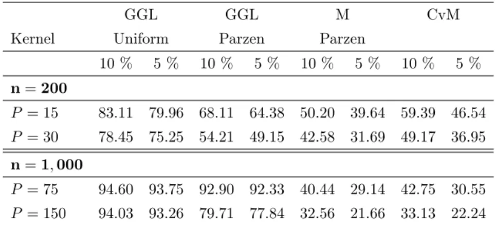
randomly from the standard normal distribution. The lag index P is set to 15 and 30 for 200 observations and 75 and 150 for 1,000 observations. Since PPk=1 2k;b = P (1 + oP(1)) when P tends to in…nity, the covariance structure of the alternatives (4.9) is described in Lemma 1. Simulation results are given in Table 3.
As implied by Proposition 2, the adaptive procedure developed in this paper outperforms the CvM and M (pbIM SE) tests for all values of P and n considered in the simulation. The higher the value of P , the
larger is the di¤erence in favor of our procedure. The di¤erence in the rejection rate can be as large as 70%. The relative poor performance of the CvM test is easily explained by the fact that the CvM statistic places more emphasis on low order autocorrelations than on higher order autocorrelation. However, the CvM test outperforms the M test for P = 15 and 30 and the two tests are equivalent for P = 75 and 150. The poor performance of the M test is again due to a low pbIM SE. Finally, for our procedure, the uniform kernel
performs better than the Parzen kernel, with a di¤erence in rejection rate that can be as large as 15% for P = 150. This result is not surprising since the Parzen kernel puts larger weight on low order autocorrelation coe¢ cients and smaller weight on higher order coe¢ cients. This contrasts with the simulation results for alternatives (4.6) showing that the choice of the kernel may a¤ect detection of speci…c alternatives.
GGL GGL M CvM Kernel Uniform Parzen Parzen
10 % 5 % 10 % 5 % 10 % 5 % 10 % 5 % n= 200 P = 15 83.11 79.96 68.11 64.38 50.20 39.64 59.39 46.54 P = 30 78.45 75.25 54.21 49.15 42.58 31.69 49.17 36.95 n= 1; 000 P = 75 94.60 93.75 92.90 92.33 40.44 29.14 42.75 30.55 P = 150 94.03 93.26 79.71 77.84 32.56 21.66 33.13 22.24
Table 3: Power of tests under small correlation coe¢ cients alternatives.
5. Applications to financial squared returns
5.1. Correction for heteroskedasticity and details of the test. To deal with the problem of het-eroskedasticity, Deo (2000), Francq, Roy and Zakoian (2005), Lobato, Nankervis and Savin (2001) and Robinson (1991b) have proposed to modify the existing tests by using a better standardization of bRj in
place of bR0as explained now. Relaxing independence of futg and assuming that fut; t 1g is a sequence of
centered martingale di¤erences, we obtain that Var Rbj = Var 1 n n jX t=1 utut+j ! = 1 n 1 j n E u 2 tu2t+j = 1 n 1 j n 2 j; where 2
jmay di¤er from R20if E u2tu2t+j 6= E u2t E u2t+j . It follows that it may be advisable to standardize
the estimated covariances bRj using ^j with ^2j =
Pn j
t=1u^2tu^2t+j=n. In our application, we consider the
modi…ed Box-Pierce statistics
BPp = n n 1X j=1 ^ Rj ^j !2 ; p 2 P.
With this de…nition, the mean and variance terms E(p), V2(p) and V2(p; p) in the de…nition of the test (2.10) can be set equal to p, 2p and 2(p p) respectively.
We consider monthly returns vt = log (Pt=Pt 1), t = 1; :::; n, of the Dow Jones Index from January
1950 to April 2008 (n = 700) and monthly returns of the Coca-Cola share from January 1962 to April 2008 (n = 555). In both cases, the returns are found to be uncorrelated. The tests are then applied to squared de-meaned returns
b
ut= (vt v)2 (vt v)2; t = 1; :::; n:
Although the mean of the returns and of the squared returns is estimated, elementary expansions show that this does not a¤ect the joint null limit distribution of the covariances. It follows that the CvM statistic has its usual null limit distribution. Similarly, the null limit distribution of BPpb is a chi-square with p degrees of freedom. In order to limit small sample impact of mean estimation, the minimal lag index p is set to 4, a
value which is slightly larger than the minimal lag index 2 used in the simulation experiments. For the Dow Jones returns, p is equal to 256 and the penalty is as in the simulation experiment, n= (2 log 6)
1=2
+ 3:2. For the Coca-Cola returns, a smaller p = 128 is considered due to a smaller sample size and the penalty is equal to n = (2 log 5)1=2+ 3:2.
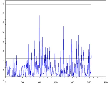
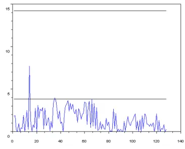
5.2. Index returns. Figure 1 below displays the standardized squared sample covariances n( bRj=bj)2, j =
1; :::; 256; of the de-meaned squared returns of the Dow Jones Index. The upper horizontal line is the 5% critical value10, 15:24, of the test based on maxj2[1;256]n( bRj=bj)2. The lower horizontal line corresponds to
1:962= 3:8416, so that 95% of the n( bR
j=bj)2, j = 1; :::; 256, should lie below this line under the null.
Figure 1: Sample standardized autocovariance of the Dow Jones Index squared monthly returns. The upper horizontal line is the 5% critical value, 15.24, of the test based on max1 j 128n( ^Rj=^j)2. The lower
horizontal is the asymptotic 95% quantile of the individual n( ^Rj=^j)2.
The observed value of n Maxj2[1;256]( ^Rj=^j)2 is below its 5% critical value. The value of the CvM
statistic is 0:31 (p-value 0:12). The M statistic, withpbIM SE= 11:33, gives a slightly smaller p-value of 0:08.
Hence all these tests accept the null at the 5% level. This conclusion contrasts with quite high percentage 12:5% of standardized squared sample correlations above the 1:962 line, which gives a negligible p-value to
the null. That the CvM and M tests do not detect may be due to the fact that high correlation coe¢ cients are mostly achieved for high lags typically larger than 70. Our selection procedure (2.8) withbp = 256 is more sensitive to the high lag behavior of the sample correlation function. Our test statistic BPpb has a value of 210 and rejects the absence of serial correlation at any reasonable statistical level.
10Since under the null of independence the n1=2Rb
j=bjare asymptotically independent standard normal, this critical value has been computed using the double exponential approximation of the maximum of p = 256 independent chi square variables with 1 degree of freedom.
5.3. Stock returns. Figure 2 reports the standardized squared sample covariances n( bRj=bj)2, j = 1; :::; 128;
of the de-meaned squared returns of the Coca-Cola stock. The upper horizontal line corresponds to the 5% critical value of the test based on maxj2[1;128]n( bRj=bj)2which has a slightly lower value of 14:18 for p = 128.
The lower horizontal line corresponds to 1:962, so that 95% of the n( bR
j=bj)2 for j = 1; :::; 128 should lie
below this line under the null.
Figure 2: Sample standardized autocovariance of Coca Cola squared monthly returns. The upper horizontal line is the 5% critical value, 14.18, of the test based on max1 j 128n( ^Rj=^j)2. The lower horizontal is the
asymptotic 95% quantile of the individual n( ^Rj=^j)2.
The sample covariance function in Figure 2 di¤ers from the function given in Figure 1 and shares some aspects with the covariance functions that can be generated by an uncorrelated process or by small alternatives (3.11). In particular, the percentage of n( bRj=bj)2above 1:962is very low, with a value of 1:56%.
Not surprisingly, the asymptotic p-value of the CvM test statistic is 0:17, so the CvM test accepts the null of absence of serial correlation at usual statistical levels. The M statistic gives a p-value larger than 0:50 for the null.
The conclusion based on the M, CvM and con…dence interval test contrasts with the conclusion based on our test which with BPbp = 121 rejects the null of absence of serial correlation at all reasonable levels. Such a high value of the test statistic may be due to the fact that many standardized covariances n( ^Rj=^j)2
are close to 1:962 for lags j 2 [30; 70]. Although this corresponds to small values for the standardized
6. Concluding remarks
The paper proposes an adaptive test for absence of serial correlation. The test is based on a new data-driven selection procedure of the smoothing parameter in the test statistics used by Box and Pierce (1970) and Hong (1996). The test can be based on simple critical values such as chi-square or normal and does not rely on bootstrap procedures than can be di¢ cult to apply in time series contexts. The selection procedure is speci…c to testing and is designed to achieve rate-optimality properties. An important theoretical …nding is that the adaptive test can consistently detect alternatives with autocorrelation coe¢ cients of order
n= o n 1=2 where n is the sample size. Such a result holds provided that the number of autocorrelation
coe¢ cients of order larger or equal to n remains large enough. The analysis of such alternatives has led us to develop a new class of so called small alternatives with autocorrelation coe¢ cients of order o n 1=2 . The
proposed test has been shown to be adaptive rate-optimal against this class of small alternatives, as well as adaptive rate-optimal against smooth alternatives, a framework previously used in Horowitz and Spokoiny (2001). The test is also consistent against Pitman local alternatives which converge to the null at a rate close or equal to the parametric rate n1=2, and against ARMA-type alternatives which converge to the null
at a rate close to the parametric rate.
The paper gives examples of alternatives with small autocorrelation coe¢ cients of order o n 1=2 which
are detected by the new test. These examples consist of high-order moving average processes with moving average coe¢ cients converging to zero at a o n 1=2 rate. Due to the small size of the coe¢ cients, standard con…dence interval techniques for the moving average or autocorrelation coe¢ cients will wrongly conclude that the serial correlation is absent. The paper shows that the Cramér-von Mises test of Durlauf (1991) is not consistent against such small alternatives either. Our simulation experiments demonstrate that the power of a data-driven version of the Hong (1996) test based on Andrews (1991) and Newey and West (1994) is also very low. Interestingly, an empirical example of monthly squared …nancial returns similarly exhibits correlation coe¢ cients which are not signi…cantly large when considered individually or when tested using the Hong (1996) or CvM tests. In contrast, our test indicates presence of autocorrelation.
References
[1] Anderson T. W. (1993). Goodness of Fit Tests for Spectral Distributions. The Annals of Statistics 21, 830–847. [2] Anderson T. W., D.A. Darling (1952). Asymptotic Theory of Certain ”Goodness of Fit” Criteria Based on Stochastic
Processes. Annals of Mathematical Statistics 23, 193–212.
[3] Andrews D. W. K. (1991). Heteroscedasticity and Autocorrelation Consistent Covariance Matrix Estimation. Economet-rica 59, 817–858.
[4] Bartlett, M.S. (1954) Problèmes de l’analyse spectrale des séries temporelles. Publications de l’Institut de Statistique de l’Université de Paris III-3 27-41.
[5] Berman, S.M. (1962). A Law of Large Numbers for the Maximum in a Stationary Gaussian Sequence. The Annals of Mathematical Statistics 33, 93-97.
[6] Box, G., D. Pierce (1970). Distribution of Residual Autocorrelations in Autoregressive-Integrated Moving Average Time Series Models. Journal of American Statistical Association 65, 1509–1526.
[7] Brillinger, D.R. (2001). Time Series Analysis: Data Analysis and Theory . Holt, Rinehart & Winston, New-York. [8] Brockwell, P.J., R.A. Davis (2006). Time Series: Theory and Methods. Second Edition, Springer.
[10] Chow, Y.S., H. Teicher (1988). Probability Theory. Independence, Interchangeability, Martingales . Second Edition, Springer.
[11] Deo, R.S. (2000). Spectral Tests of the Martingale Hypothesis under Conditional Heteroscedasticity. Journal of Econo-metrics 99, 291-315.
[12] Donoho, D. and J. Jin (2004). Higher criticism for detecting sparse heterogeneous mixtures. The Annals of Statistics 32 962–994
[13] Durlauf, S.N. (1991). Spectral Based Testing of the Martingale Hypothesis. Journal of Econometrics 50, 355-376. [14] Ermakov, M.S. (1994). A Minimax Test for Hypotheses on a Spectral Density.Journal of Mathematical Sciences 68,
475–483. Translated from Zapiski Nauchnykh Seminarov Leningradskogo Otdeleniya Matematicheskogo Instituta im. V. A. Steklova Akademii Nauk SSSR 184, 115— 125, 1990.
[15] Fan, J. (1996). Test of Signi…cance Based on Wavelet Thresholding and Neyman’s Truncation. Journal of the American Statistical Association 91, 674–688.
[16] Fan, J., Q. Yao (2005). Nonlinear Time Series. Nonparametric and Parametric Methods. Springer.
[17] Francq, C. , R. Roy and J.M. Zakoian (2005). Diagnostic Checking in ARMA Models With Uncorrelated Errors. Journal of the American Statistical Association, 100, 532–544.
[18] Golubev, G.K., M. Nussbaum and H.H. Zhou (2009). Asymptotic Equivalence of Spectrum Density Estimation and Gaussian White Noise. Document Paper. Forthcoming in The Annals of Statistics.
[19] Grenander, U., M. Rosenblatt (1952). On Spectral Analysis of Stationary Time-series. Proceedings of the National Academy of Sciences U.S.A. 38 519-521.
[20] Guay, A., E. Guerre (2006). A Data-Driven Nonparametric Speci…cation Test for Dynamic Regression Models. Econo-metric Theory 22, 543–586.
[21] Guerre, E., P. Lavergne (2005). Rate-Optimal Data-Driven Speci…cation Testing for Regression Models. The Annals of Statistics 33, 840-870.
[22] Hong, Y. (1996). Consistent Testing for Serial Correlation of Unknown Form. Econometrica 64, 837–864.
[23] Hong, Y. (1999). Hypothesis Testing in Time Series via the Empirical Characteristic Function: A Generalized Spectral Density Approach. Journal of the American Statistical Association 94, 1201–1220.
[24] Hong, Y., Y.J Lee. (2005). Generalized Spectral Tests for Conditional Mean Models in Time Series with Conditional Heteroscedasticity of Unknown Form. Review of Economic Studies 72, 499–541.
[25] Horowitz, J.L., V.G. Spokoiny (2001). An Adaptive, Rate-Optimal Test of a Parametric Mean-Regression Model Against a Nonparametric Alternative. Econometrica 69, 599–631.
[26] Ingster, Y.I. (1993). Asymptotically Minimax Hypothesis Testing for Nonparametric Alternatives. I, II, III. Mathematical Methods of Statistics 2, 85–114, 171–189 and 249–268.
[27] Ingster, Y.I. (1997). Some problems of hypothesis testing leading to in…nitely divisible distribution. Mathematical Methods of Statistics 6, 647–669
[28] Lobato, I., J.C. Nankervis and N.E. Savin (2001). Testing for Autocorrelation Using a Modi…ed Box-Pierce Q Test. International Economic Review, 42, 187–205.
[29] Lütkepohl, H. and M. Krätzig (2004). Applied Time Series Econometrics. Cambridge University Press.
[30] Newey, W.K. and K. West (1994). Automatic Lag Selection in Covariance Matrix Estimation. Review of Economic Studies, 61, pp. 631–653.
[31] Paparoditis, E. (2000). Spectral Density Based Goodness-of-Fit Tests for Time Series Models. Scandinavian Journal of Statistics 27, 143–176.
[32] Pollard, D. (2002). A User’s Guide to Measure Theoretic Probability . Cambridge University Press.
[33] P½Otscher, B.M. (2002). Lower Risk Bounds and Properties of Con…dence Sets for Ill-Posed Estimation Problems with Applications to Spectral Density and Persistence Estimation, Unit Roots and Estimation of Long Memory Parameters. Econometrica 70, 1035-1065.
[35] Robinson, P.M. (1991a). Automatic Frequency Domain Inference on Semiparametric and Nonparametric Models. Econo-metrica 59, 1329-1363.
[36] Robinson, P.M. (1991b). Testing for Strong Serial Correlation and Dynamic Conditional Heteroskedasticity in Multiple Regression. Journal of Econometrics 47, 67-84.
[37] Romano, J.P. and L.A. Thombs (1996). Inference For Autocorrelations Under Weak Assumptions. Journal of the American Statistical Association 91, 590-600.
[38] Shorack, G.R. (2000). Probability for Statisticians. New York: Springer-Verlag.
[39] Spokoiny, V. G. (1996). Adaptive Hypothesis Testing Using Wavelets. The Annals of Statistics 24, 2477–2498.
Appendix A: proofs of main results
This section contains the proofs of the results of Section 3. For j = 1; : : : ; n 1 and p = 1; : : : ; n, let e Rj= 1 n nXjjj t=1 utut+jjj and Sep= n n 1 X j=1 K2 j p Re 2 j
be the sample covariances and the test statistics computed using u1; :::; un. In this section, C and C0 are
constants that may vary from line to line but only depend on the constants of the assumptions. Notation [ ] is used for the integer part of a real number.
We …rst state some intermediary results that are used in the proofs of our main results. These interme-diary results are proven in Appendix B. Lemma A.1 gives the order of standardization terms E(p), E(p; p), V (p) and V (p; p). Propositions A.1 and A.2 deal with the impact of the estimation of . Proposition A.3 is used to study the asymptotic null behavior of the test. Propositions A.4 and A.5 together with the lower bounds (2.11) are the key tools for the derivation of the consistency results.
Lemma A.1. Suppose that Assumption K holds and that p=n 1=2.
(i) There exists a constant C > 1 such that, for q = 1; 2 and for any p p p, p C n 1X j=1 1 j n q K2q j p Cp; p C n 1X j=1 K2q j p Cp; V 2(p; p) Cp; and E(p; p) n 1 X j=1 K2 j p K 2 j p Cp 1=2V (p; p):
(ii) Under Assumption P, for all n,
V (p; p) C(p p)1=2 for all p 2 P; V (p; p) Cp1=2 for p 6= p 2 P; E(p; p) 0 for all p 2 P: Proposition A.1. Suppose the sequence fut;ng satis…es Assumption M. If
1 C R0;n C and +1 X j1;j2;j3= 1 j n(0; j1; j2; j3)j C
then for any jn= o(n),
b Rjn b R0 =Rjn;n R0;n + OP 0 B @ 0 @n 1 2n X j=0 Rj;n R0;n 21 A 1=21 C A + OP n 1=2 :