HAL Id: hal-00592055
https://hal.archives-ouvertes.fr/hal-00592055
Submitted on 11 May 2011
HAL is a multi-disciplinary open access
archive for the deposit and dissemination of sci-entific research documents, whether they are pub-lished or not. The documents may come from teaching and research institutions in France or
L’archive ouverte pluridisciplinaire HAL, est destinée au dépôt et à la diffusion de documents scientifiques de niveau recherche, publiés ou non, émanant des établissements d’enseignement et de recherche français ou étrangers, des laboratoires
Scheduling Problem with Blocking Constraints
Yazid Mati, Chams Lahlou, Stephane Dauzere-Peres
To cite this version:
Yazid Mati, Chams Lahlou, Stephane Dauzere-Peres. Modelling and Solving a Practical Flexible Job-Shop Scheduling Problem with Blocking Constraints. International Journal of Production Research, Taylor & Francis, 2010, pp.1. �10.1080/00207541003733775�. �hal-00592055�
For Peer Review Only
Modelling and Solving a Practical Flexible Job-Shop Scheduling Problem with Blocking Constraints
Journal: International Journal of Production Research Manuscript ID: TPRS-2009-IJPR-0323.R2
Manuscript Type: Original Manuscript Date Submitted by the
Author: 11-Feb-2010
Complete List of Authors: Mati, Yazid; Al-Qassim University, College of Business & Economics Lahlou, Chams; Ecole des mines de Nantes, Automatic Control and Industrial Engineering
Dauzere-Peres, Stephane; Ecole des Mines de Saint-Etienne, Site Georges Charpak, Centre Microelectronique de Provence
Keywords: JOB SHOP SCHEDULING, GENETIC ALGORITHMS, DESIGN Keywords (user): flexible, blocking
For Peer Review Only
International Journal of Production Research Vol. 00, No. 00, 00 Month 200x, 1–18
RESEARCH ARTICLE
Modelling and Solving a Practical Flexible Job-Shop Scheduling Problem with Blocking Constraints
Yazid Matia, Chams Lahloub∗ and St´ephane Dauz`ere-P´er`esc
aAl-Qassim University. College of Business & Economics. Almelaida, P.O. Box 6633,
Kingdom of Saudi Arabia. Email: [email protected].
bEcole des Mines de Nantes - IRCCyN CNRS-UMR 6597. 4, rue A. Kastler. La
Chantrerie – BP 20722, F-44307 Nantes Cedex 3 – France.
cEcole des Mines de Saint-Etienne, Site Georges Charpak – Centre Micro´electronique de
Provence, 880 avenue de Mimet, F-13541 Gardanne – France. Email: [email protected]
(Received 00 Month 200x; final version received 00 Month 200x)
This paper aims at presenting the study of a practical job-shop scheduling problem we mod-elled and solved when helping a company to design a new production workshop. The main characteristics of the problem are that some resources are flexible, and blocking constraints have to be taken into account. The problem and the motivations for solving it are detailed. The modelling of the problem and the proposed resolution approach, a genetic algorithm, are described. Numerical experiments on real data are presented and analysed. We also show how these results were used to support choices in the design of the workshop.
Keywords: Job-shop scheduling, genetic algorithm, flexible, blocking, design.
∗Corresponding author. Email: [email protected]
1 2 3 4 5 6 7 8 9 10 11 12 13 14 15 16 17 18 19 20 21 22 23 24 25 26 27 28 29 30 31 32 33 34 35 36 37 38 39 40 41 42 43 44 45 46 47 48 49 50 51 52 53 54 55 56 57 58 59 60
For Peer Review Only
1. Introduction
Designing a manufacturing system involves complex decisions with conflicting ob-jectives such as cost reduction, high equipment utilization and customer satisfac-tion. One of the important issues is the selection of the proper equipment type and number. In modern manufacturing systems, machines are more and more flexible, and choosing the adequate type is crucial to handle the variety of possible prod-ucts, demand fluctuations and machine failures. Further, determining the right equipment number helps reducing the procurement and maintenance costs while increasing the equipment utilization.
This paper discusses the problem of selecting machines in a workshop where key components of aircrafts are produced. With the increase of demand and in order to satisfy customers while minimizing costs, the company under consideration was setting a new workshop that could make different part types on the same set of machines. The main challenge the company had to face was the determination of an adequate configuration of the workshop, in order to minimize the cycle times of products. After a first analysis carried out at the company, focusing on demand forecast, a first configuration of the workshop was proposed. In this configuration, products have to go through workstations, and there is one machine in each work-station. The company was interested in evaluating various choices before building the workshop such as: the number of entrant workstations, the functions of some workstations (i.e. the machine type in these workstations), etc.
In the classical literature on equipment selection (see Chen 1999, for instance), aggregate models are proposed and solved in which the details of the actual pro-cessing of jobs is not considered. In our approach, and because the scheduling con-straints are important, we needed to solve a more detailed model that integrates detailed scheduling features to be sure that the design choices were correct. Our problem is thus formulated as a scheduling problem with several possible scenar-ios for the design of the workshop. The resulting scheduling problem is a complex shop problem with a material handling system for transporting products, resource flexibility, lack of buffer space between machines, etc.
Flexible shop scheduling problems have attracted many researchers who mainly addressed the shop case with multi-purpose machines (also called flexible job-shop), in which an operation may be processed on several machines in a given set, and one of them must be selected. Complexity results are given by Brucker and Schlie (1990), Mati and Xie (2004) for the two-job case. For the flexible job-shop with several jobs, various heuristics are proposed. Most of them use a disjunctive graph for representing feasible solutions and a tabu search heuristic to guide the search. Among these heuristics we may cite the hierarchical approach of Paulli (1995) and the integrated approach of Dauz`ere-P´er`es and Paulli (1997). A heuristic based on genetic algorithms is developed in Chan et al. (2006). This approach is used in an iterative approach to evaluate different flexibility levels of assignment of operations to machines. A generalization to the case where an operation may be processed on several resources simultaneously (multi-resource) is done by Dauz` ere-P´er`es et al. (1998), Mati and Xie (2008a). In the first paper, a tabu search heuristic is proposed using the disjunctive graph representation. The second paper presents a greedy heuristic that schedules jobs one after another according to a job sequence. A genetic algorithm is used to optimize the job sequence.
The blocking constraint arises in production environment where buffer capacity between workstations is limited. Scheduling problems that take into account this constraint are not abundant and the majority of existing studies concentrates on the flow-shop and hybrid flow-shop scheduling problems. A survey on blocking
con-1 2 3 4 5 6 7 8 9 10 11 12 13 14 15 16 17 18 19 20 21 22 23 24 25 26 27 28 29 30 31 32 33 34 35 36 37 38 39 40 41 42 43 44 45 46 47 48 49 50 51 52 53 54 55 56 57 58 59 60
For Peer Review Only
straints is proposed by Hall and Sriskandarajah (1996). For the flow-shop problem, Grabowski and Pempera (2007) use the disjunctive graph model for modelling and propose tabu search heuristics for solving the problem. A genetic algorithm is pro-posed by Caraffa et al. (2001) for minimizing the makespan. A branch and bound method is proposed by Ronconi (2008) and some complexity results are given by Martinez et al. (2006) for a new type of blocking constraint. For the hybrid flow-shop problem, some heuristic methods are proposed by Wang and Tang (2008), Wardono and Fathi (2004) and exact methods are investigated by Sawik (1995, 2000).
Considering blocking constraints in job-shop environments leads to a control problem called deadlock situation. A system deadlock is a situation that arises when the flow of products is permanently inhibited and/or operations on products cannot be performed. For example, in a robotic cell, a deadlock arises if the robot carries a part to a machine which is working on another part. Under such a situation, the robot cannot unload the part since the machine is not free and needs the robot to download the part it is working on.
Various solutions have been proposed to handle deadlock situations in auto-mated manufacturing systems (Chu and Xie 1997): deadlock prevention, detection and avoidance methods. The majority of previous studies that deal with schedul-ing and deadlock issues uses Petri nets and reachability graphs to obtain optimal solutions (Lee and DiCesare 1994, ElMaraghy and ElMekkawy 2002). Mati et al. (2001a,b) propose two heuristics for solving the job-shop scheduling problem with multi-resource operations. The first heuristic uses a greedy heuristic and genetic al-gorithms. The second heuristic makes use of the disjunctive graph and tabu search. Integer linear programming models are proposed in Gomes et al. (2005) to schedule flexible job shops under limited intermediate buffers. These models are validated on realistic examples using commercial mathematical programming software. Various characteristics make our problem more complex. A deadlock-free reactive schedul-ing approach is proposed in Fahmy et al. (2009), which aims at answerschedul-ing in real time to the occurrence of a variety of possible disruptions in flexible job shops.
This paper formulates a practical equipment selection problem as a complex scheduling problem and presents a heuristic approach for solving it. The rest of the paper is organized as follows. Section 2 gives a detailed description of the problem encountered by the company, in particular the features of the production environ-ment. Section 3 presents how the problem was modelled, with the assumptions made together with the company. Our resolution method is then described in Sec-tion 4. Numerical experiments are shown in SecSec-tion 5, together with the analysis that was performed. Finally, Section 6 ends the paper with some conclusions and perspectives.
2. Description of the problem
The problem of selecting equipment for designing a production workshop is for-mulated as a scheduling problem that is solved for each design scenario of the workshop. This approach is possible because the number of alternatives is lim-ited. This section describes the various features of the production environment and the connection between the resulting scheduling problem and those studied in the scheduling literature.
The company has a set of N products (8 in the specific setting we are con-sidering) J = {J1, J2, . . . , JN} that must be performed in the planning horizon
H. Each product Ji must be performed in a number of units that differs from
one product to another. There are 8 machines (i.e. workstations) in the workshop
1 2 3 4 5 6 7 8 9 10 11 12 13 14 15 16 17 18 19 20 21 22 23 24 25 26 27 28 29 30 31 32 33 34 35 36 37 38 39 40 41 42 43 44 45 46 47 48 49 50 51 52 53 54 55 56 57 58 59 60
For Peer Review Only
M = {M1, M2, . . . , M8}, where machines M1 and M3 (resp. M2 and M4) are of the
same type (i.e. can process the same set of operations). Each machine can perform no more than one product at a time and is assumed to be continuously available during the planning horizon. Five different tasks T ∈ {T1, . . . , T5} are performed
in the production workshop. Task T1 can be carried out by machines M2 or M4.
Task T2 can be performed by any machine in the set {M1, M3, M5}, where M5is an
optional machine that the company could acquire or not. Tasks T3, T4 and T5 are
performed on machines M6, M7 and M8, respectively. The layout of the workshop
is described in Figure 1.
The products enter the workshop via a loading workstation (called entrant work-station in this paper) where they are put on pallets. Task T1 is the first operation
to be performed for each product. The remaining sequences of operations slightly vary from one product type to another, but the estimated processing times can be very different. Some tasks are not needed for some products and others are repeated several times. The sequence of tasks is (T1, T2, T3, T2, T1, T2, T3, T4, T5)
for products J1, J2 and J3, (T1, T2, T1, T2, T3, T4, T5) for product J4, and (T1, T2,
T1, T2, T4, T5) for products J5 through J8.
Due to the size and weight of the products, there is no buffer space for storing products between machines. Thus, if a product finishes its processing on a machine and the machine on which the product has to be processed next is occupied, then the product has to wait on the current machine, thus blocking it for performing other products. This feature is referred in the scheduling literature to as the block-ing constraint (Hall and Sriskandarajah 1996). It is also called the hold-while-wait constraint by authors who address the scheduling and deadlock avoidance problems (Mati et al. 2001b).
With the above features, and according to the scheduling literature, the problem can be seen as a flexible job-shop scheduling problem with blocking constraints, for which some operations have several possibilities to be performed and the rep-etition of operations is allowed, i.e. the same operation may appear several times in the sequence of a product. An important feature that makes this scheduling problem different from other problems with blocking investigated in the literature is that poor sequencing of machines may lead to undesirable deadlocks (Mati et al. 2001a,b). More precisely, let us consider two products P1 and P2 with two
oper-ations each. The first operation of P1 can be performed by M1 or M2 and the
second operation by M3. The first operation of P2 is performed by M3 and the
second by M2. Thus, if one decides to assign M2 to the first operation of P1 and
to allow the first operations of the two products to be performed simultaneously, then a deadlock situation occurs since P1 cannot move to its second operation (M3
is occupied by P2) and P2 cannot progress to its second operation (M2 is occupied
by P1).
Moreover, the manufacturing environment is characterized by the following fea-tures that lead to an even more complex scheduling problem.
• Limited number of pallets. Products to be produced are put on pallets at the loading (or entrant) workstation. After having visited all necessary machines in the manufacturing process, a product is removed from the pallet on which it is attached, and the pallet is moved to the entrant workstation for processing a new product. Due to the cost of a pallet, only a limited number is allowed limiting the number of products in the workshop at the same time.
• Material handling. The workstations are linked by an Automated Material Han-dling System (AMHS) that moves the products between the machines, and be-tween the machines and the loading/unloading (or entrant) workstations. The AMHS can handle only one product at a time. When the AMHS moves a product
1 2 3 4 5 6 7 8 9 10 11 12 13 14 15 16 17 18 19 20 21 22 23 24 25 26 27 28 29 30 31 32 33 34 35 36 37 38 39 40 41 42 43 44 45 46 47 48 49 50 51 52 53 54 55 56 57 58 59 60
For Peer Review Only
on the machine on which it is processed next, this machine must be available. This is a no-wait constraint that prevents the AMHS to hold products.
• Storage on machines. If the machine that processes the next operation of a product is occupied then the product can be stored on any empty machine. This alternative minimizes the blocking times and improves the utilization of critical machines.
• Negative time lags. Some operations can be started even though the preceding operation on the routing is not yet completed. This time corresponds to the preparation of the machine by an operator, and represents about 5% of the processing time.
The company was interested in evaluating various choices that had to be made before building the workshop. The first choice concerns the number of entrant work-stations from which products are brought into the workshop. Since the processing of products begins with task T1, it could be possible, at an additional investment
cost, to also use M4 as an entrant workstation, instead of only M2. The second
choice concerns the need of purchasing a new workstation (i.e. a new machine M5)
and thus changing the functions of some workstations by modifying manufacturing processes. The last choice concerns the determination of the right number of pallets to be used in the workshop. A smaller number of pallets means less products in the workshop, which may decrease the utilization of machines and therefore increases the total time to process all products. On the other hand, more pallets may lead to more products in the workshop and thus increased congestion due to blocking constraints.
We shall show in the next sections how we modelled and solved the scheduling problem to help the company answer these three questions.
3. Modelling the problem
Taking into account all the features of the production environment results in a complex scheduling model. In order to solve the problem, some constraints were relaxed, validated by the company. This section first discusses how the constraints are modelled and then specifies those that are relaxed. The manufacturing processes of jobs are modified. In what follows, we use the following notation to describe an operation Oi,j of a product Ji: (S1, . . . , St, pi,j), where Sk ⊂ M is the kth set
of resources that can be used to perform Oi,j, and pi,j is the processing time
which does not depend on the chosen set of resources. As it will be shown below, the resources in our problem are the machines, the Automated Material Handling System (AMHS) and the pallets.
Let us illustrate our modelling choices in the following subsections on two con-secutive operations Oi,j and Oi,j+1 of a product Ji described by the routing (1):
Ji ≡ . . . ; ({M1}, pi,j); ({M2}, {M3}, pi,j+1); . . . (1)
This means that, at operation Oi,j, the product Ji must be processed on machine
M1 with a processing time of pi,j and, at operation Oi,j+1, can be processed either
on machine M2 or on machine M3 with a processing time of pi,j+1.
3.1 Storage on machines
To integrate the possibility of storing Ji between Oi,j and Oi,j+1 on machines M4
or M5, a waiting operation Oi,j+ = ({M1}, {M4}, {M5}, 0) is added between Oi,j
and Oi,j+1. Machines M1 is integrated in the set of alternative machines to express
1 2 3 4 5 6 7 8 9 10 11 12 13 14 15 16 17 18 19 20 21 22 23 24 25 26 27 28 29 30 31 32 33 34 35 36 37 38 39 40 41 42 43 44 45 46 47 48 49 50 51 52 53 54 55 56 57 58 59 60
For Peer Review Only
the fact that Ji can also wait on this machine. If one of the machines that can
perform Oi,j+1 is empty, then Ji can move to Oi,j+1 by advancing instantaneously
to Oi,j+ on machine M1 and then to Oi,j+1. The new manufacturing process of Ji
is given by the routing (2):
Ji ≡ . . . ; ({M1}, pi,j); ({M1}, {M4}, {M5}, 0); ({M2}, {M3}, pi,j+1); . . . (2)
3.2 Material handling
The AMHS can be explicitly integrated by adding a transportation operation be-tween any two consecutive operations. The added operation (noted j+ in the ex-ample below) needs the AMHS and the processing time corresponds to the time needed for moving products. Adding this information to the manufacturing process of job Ji leads to the one given by the routing (3) where A denotes the AMHS:
Ji ≡ . . . ; ({M1}, pi,j); ({A}, tj,j+); ({M1}, {M4}, {M5}, 0); ({A}, tj+,j+1); . . . (3)
where tj,k is the time needed for the AMHS to bring product Ji from the
worksta-tion selected for operaworksta-tion Oi,j to the workstation selected for operation Oi,k. This
time depends on the distance between these workstations in the workshop.
3.3 Pallets
Up to this point, every operation needs only one resource to be processed. However, it is necessary to take into account the fact that a pallet is needed for each product from the beginning until the end of its process. Hence, the pallets are modelled as a resource R which is available in a given number of units. The manufacturing process is then modelled by the routing (4):
Ji≡ . . . ; ({M1, R}, pi,j); ({A, R}, tj,j+); ({M1, R}, {M4, R}, {M5, R}, 0); . . . (4)
The fact that the pallet moves to the entrant workstation after completing the product is modelled by adding an operation at the end of the routing of each product. This operation needs the pallet and the AMHS with a processing time equal to the time needed to move to the entrant workstation.
Note that if the number of pallets is equal to one, the scheduling problem be-comes trivial and the solution consists of bringing products one after another in the workshop. If the number of pallets is equal to the number of machines, the problem is equivalent to a flexible job-shop scheduling problem with blocking and thus pallets can be omitted.
3.4 The relaxed constraints
The no-wait constraint that prevents the AMHS to hold the products is always fulfilled since the schedules generated by the solving method are feasible. Otherwise there may be a case where the AMHS moves a product from a given machine Mi
and finds the next machine Mj already occupied. This is a deadlock situation since
Mj can only be released by the AMHS.
The first constraint that is relaxed in our modelling and solving method is the transportation time that depends on the distance between machines. We use an average time of the transportation times between all workstations of the workshop. After solving the scheduling problem, we recalculate the starting and finishing times of operations by integrating the actual values of the transportation times. Of
1 2 3 4 5 6 7 8 9 10 11 12 13 14 15 16 17 18 19 20 21 22 23 24 25 26 27 28 29 30 31 32 33 34 35 36 37 38 39 40 41 42 43 44 45 46 47 48 49 50 51 52 53 54 55 56 57 58 59 60
For Peer Review Only
course, if a waiting operation uses the same previous machine in the manufacturing process (for instance M1 in the routing (4)) then the moving time is equal to zero.
The second relaxed constraint is the time lags between two consecutive operations on the routing. We solve the problem without these times and, after finding a solution, a shifting procedure is called to find the actual starting and finishing times of operations.
The third relaxed constraint is related to the limited number of pallets np.
Inte-grating this feature in our scheduling model is difficult for the resolution method of (Mati and Xie 2008b), which will be used for evaluating the fitness of chromo-somes in the proposed algorithm. One way would be to model each pallet as a separate resource and to integrate flexibility each time an operation needs a pal-let. This solution is not convenient as it leads to a huge number of alternative sets (Dauz`ere-P´er`es and Paulli 1997). In our case, we assume that the number of pallets is infinite and, during the search process, we save the best schedule with a given maximum number of pallets (np ∈ {3, 4, 5, 6, 7} in our numerical experiments).
The number of pallets required for a given schedule is determined by finding, over the entire schedule, the maximum number of jobs progressing in parallel in the workshop.
With the above modelling and simplification in mind, the resulting scheduling problem that is solved is a multi-resource job-shop scheduling problem with re-source flexibility and blocking, in which an operation may need more than one resource. The AMHS is modelled as a real resource that must be taken into ac-count when building a schedule.
4. Solving the problem
One way for tackling the problem is to model it as a mixed integer linear program-ming model and to solve it using a commercial solver. Computational experiments carried out by Mati and Xie (2008b) show that commercial solvers are not able to provide reasonably good solutions for the flexible job-shop scheduling problem with blocking constraints, even for instances with less than 10 jobs and 5 machines. The method used in this paper to answer the questions of the company is an efficient genetic algorithm that uses the greedy procedure proposed by Mati and Xie (2008b) for evaluating the fitness of chromosomes. In this section, genetic algorithms are first briefly described. Then the basic parameters of our genetic algorithm are discussed, including the crossover and mutation operators and the strategy for population management. The method used for evaluating the fitness of the chromosomes is also recalled.
4.1 A brief description of genetic algorithms
Genetic algorithms are population-based procedures that start from an initial pop-ulation containing a set of feasible solutions represented by chromosomes. The first question to answer when using genetic algorithms is the chromosome encoding (or encoding scheme). There are two types of encoding, the direct and indirect encod-ing, and the selection of the suitable type depends on the characteristics of the problem. In the direct encoding, a chromosome describes a solution whereas, in the indirect encoding, the chromosome contains information that is used to build a solution. Genetic algorithms iteratively apply genetic operators to replace the cur-rent population by a new and hopefully improved population. The first operator is the crossover operator that combines the characteristics of two selected
chromo-1 2 3 4 5 6 7 8 9 10 11 12 13 14 15 16 17 18 19 20 21 22 23 24 25 26 27 28 29 30 31 32 33 34 35 36 37 38 39 40 41 42 43 44 45 46 47 48 49 50 51 52 53 54 55 56 57 58 59 60
For Peer Review Only
somes to generate one or several offsprings. Chromosomes may also be submitted to a mutation operator that consists of a small perturbation of the genes. The purpose of mutation is to prevent the search process from being trapped in local optima if chromosomes in the population become too similar. Genetic algorithms also require a suitable mechanism for population management that decides which chromosomes are selected at each generation for applying the crossover operator. It also requires a fitness function that represents a measure of the quality of each chromosome.
To describe our genetic algorithm, we present below the different parameters of the algorithm, which are fairly standard except the fitness evaluation function that is based on a greedy procedure proposed by Mati and Xie (2008b).
4.2 Parameters of our genetic algorithm
Chromosome encoding. In order to exploit standard crossover operators and to keep the feasibility of the solutions in the reproduction process, we use an indirect encoding in which a chromosome contains an n-string corresponding to a permu-tation of all integers from 1 to n. Each gene in the chromosome represents a job (product). The chromosome is then represented by a vector that gives the preference list for the treatment of all jobs. This list is used, by the fitness function described bellow, to build the actual schedule associated to the chromosome.
Initial population. In many implementations of genetic algorithms, a good start-ing population is important for the success of the algorithm. In our case, this population is constructed in a very simple way by randomly generating the chro-mosomes. However, we have found that this generally leads to a popu-lation with a very poor quality. Since it is not easy to generate a good initial population we have focused on improving it, mainly by increasing the diversity of chromosomes during the population management phase, as explained below. The size of the population is set to 20 chromosomes. This population size was fixed through numerical experiments conducted on academic test instances.
Chromosome evaluation. A greedy heuristic proposed by Mati and Xie (2008b) is employed to evaluate the chromosomes. This heuristic is recalled below.
Population management. There are two common strategies to manage the population: population replacement and incremental replacement. In the first case, the new population contains only chromosomes created by crossover and mutations operators, whereas, in the second case, only one chromosome of the parents is replaced with a generated chromosome. The population replacement has been preferred in our application since it allows a high population diversity, allowing the greedy heuristic to start from diverse chromosomes. A large part of the solution space can then be explored and hence the quality of the initial population can be improved. For selecting pairs of parents to be crossed, the simplest and most used roulette wheel selection is applied, which uses a distribution on the current population that depends on the fitness of the solutions. The probability of each chromosome to be selected is directly proportional to its fitness value.
Crossover and mutation operators. A general and suitable operator for crossover, in case of representing chromosomes by permutations, is the partially mapped crossover. This crossover has been applied successfully on many scheduling problems, and more specifically on shop problems. The crossover consists of randomly selecting two cut positions in parents
chromo-1 2 3 4 5 6 7 8 9 10 11 12 13 14 15 16 17 18 19 20 21 22 23 24 25 26 27 28 29 30 31 32 33 34 35 36 37 38 39 40 41 42 43 44 45 46 47 48 49 50 51 52 53 54 55 56 57 58 59 60
For Peer Review Only
somes, mapping the portion of one parent located between these positions onto the other parent, and then exchanging the remaining information (see Goldberg and Lingle (1985)). After using the crossover operator, a mutation operator is applied that deletes a randomly selected job from its current position in the chromosome and inserts it at another randomly selected position. One of the advantages of this mutation operator is its good ability to modify the chromosomes and thus to diversify the population. The crossover operator is applied with a probability equal to 0.9, and the mutation probability is equal to 0.05. These values are standard for scheduling problems and, as for the population size, have been validated on academic test instances.
Stopping criterion. The genetic algorithm terminates after a fixed number of gen-erations. This number has been set to 1,000 through experiments on the industrial data sets. Moreover, if no improvement of the fitness function is done after 200 generations, the algorithm is also stopped.
4.3 Fitness evaluation
The fitness function evaluates the quality of the chromosomes and plays a ma-jor role in the selection process. The solution method proposed by Mati and Xie (2008b) is used to measure the fitness of the chromosomes. This method is a greedy heuristic that schedules jobs consecutively according to the job sequence provided by the chromosome. It starts by optimally scheduling the two first jobs using a poly-nomial algorithm, called geometric approach, that reduces the scheduling problem to a shortest path problem in a two-dimensional plane with obstacles. After obtain-ing the optimal schedule for the two jobs, a combined job is defined by combinobtain-ing into a single operation the operations that are performed in parallel. Resource as-signment and operation sequencing decisions of scheduled jobs will not be modified. The geometric approach then solves the scheduling problem of the combined job and the next job in the order of the chromosome. The resulting schedule is again used to define a combined job, and the process continues until all jobs are sched-uled. The makespan of the final schedule corresponds to the fitness evaluation of the chromosome. For a detailed description of the greedy heuristic for solving shop scheduling problems, the reader is referred to Mati et al. (2001a), Mati and Xie (2008a,b).
5. Numerical experiments and analysis
We only present and discuss the results obtained on scenarios with 5 or 6 pallets since the remaining scenarios (with 3, 4 and 7 pallets) give solutions with larger total completion times and waiting times. The computational experiments were conducted on a one-month horizon, during which the workshop must produce in total 30 units of products (see the units per product in Table 1), and 323 hours of work per month (the workshop is open 17 hours per day and 19 days per month). The genetic algorithm was implemented in C++, and the experiments were ran on a Pentium IV (2 GHz). Each scenario took about 10 minutes of CPU time.
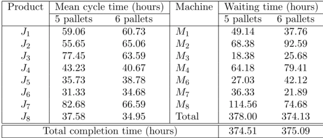
The combination of the three parameters (i.e. without or with one new worksta-tion, one or two entrant workstations, five or six pallets) led us to define 8 scenarios. The results for the scenarios are detailed in Tables 2 through 5 and discussed be-low. For each scenario, the tables show the mean cycle time per product, the total waiting time per machine and the total completion time of all products. The cycle time is the time the unit of a product stayed in the workshop (i.e. completion time
1 2 3 4 5 6 7 8 9 10 11 12 13 14 15 16 17 18 19 20 21 22 23 24 25 26 27 28 29 30 31 32 33 34 35 36 37 38 39 40 41 42 43 44 45 46 47 48 49 50 51 52 53 54 55 56 57 58 59 60
For Peer Review Only
minus arrival time), and the mean cycle time is provided for the number of units of each product.
5.1 Scenarios with no new workstation
With one entrant workstation, the total completion time is 374.51 hours (respec-tively 375.09 hours) if 5 pallets (resp. 6 pallets) are used. The solutions are detailed in Table 2. It is interesting to note that, in this configuration, allowing one more pallet only slightly improves the total waiting time on the machines.
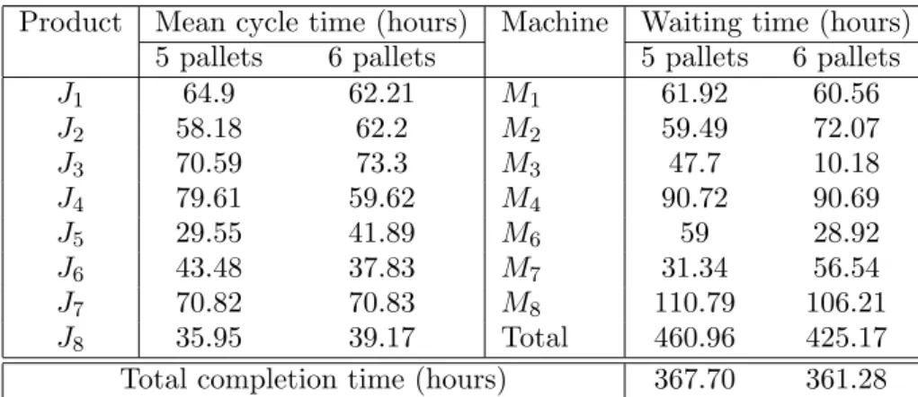
With two entrant workstations, the total completion time is reduced to 367.70 hours (resp. 361.28 hours) if 5 pallets (resp. 6 pallets) are used. As shown in the solutions of Table 3, adding one more pallet improves more the total waiting time than in the previous case. The gain is equal to 3.87 (i.e. 378 - 374.13) in the previous case and equal to 35.79 (i.e. 460.96 - 425.17) in this case.
It must be noted that using two entrant workstations instead of one leads to an improvement of the total completion time (ranging from 7 to 14 hours, i.e. less than one working day), but also to much larger waiting times, in particular when only 5 pallets are used. This can be explained by the fact that, when entrant workstations are not at all bottlenecks, arriving products are quickly pushed forward in the workshop.
5.2 Scenarios with a new workstation
With one entrant workstation, the total completion time is 369.75 hours (resp. 354.91 hours) if 5 pallets (resp. 6 pallets) are used. Hence, using 6 pallets is clearly much better and, as shown in Table 4, also leads to drastic improvements of the total waiting time (from 517.35 hours to 430.63 hours).
With two entrant workstations, the total completion time is reduced to 345.38 hours (resp. 332.16 hours) if 5 pallets (resp. 6 pallets) are used. Again, the solutions in Table 5 show that using 6 pallets also improves the total waiting time.
Using two entrant workstations reduces the total waiting time and the total completion time : the gain on the total completion time ranges from 22 hours to 24 hours (369.75 - 345.38 = 24.37 hours in case of 5 pallets, and 354.91 - 332.16 = 22.75 hours in case of 6 pallets), i.e. more than 1 working day. It is interesting to note that, contrary to the case without a new workstation, the total waiting time does not increase with two entrant workstations. This is because the capacity of the workshop has increased, and thus it can handle the products that are sent by the entrant workstations.
5.3 Answers to the questions of the company
According to the results presented in the previous subsections, our answers to the questions of the company were the following:
• It is always better to have two entrant workstations, although the improvement is really interesting, given the investment, only if one new workstation is added. • Adding a new workstation is interesting, but should be coupled with two en-trant workstations. The gain (over the scenario with one enen-trant workstation) on the total completion time is 22.75 hours (with two entrant workstations and 6 pallets), i.e. more than 1.5 days, and 101.18 hours on the total waiting time. • The workshop should be equipped with 6 pallets with either two entrant
work-stations or one new workstation.
1 2 3 4 5 6 7 8 9 10 11 12 13 14 15 16 17 18 19 20 21 22 23 24 25 26 27 28 29 30 31 32 33 34 35 36 37 38 39 40 41 42 43 44 45 46 47 48 49 50 51 52 53 54 55 56 57 58 59 60
For Peer Review Only
If one considers the possible configurations, the results of the experiments show that the worst configuration is to use one entrant workstation without a new work-station. An improved configuration is to use either two entrant workstations but no new workstation, or one new workstation but only one entrant workstation. How-ever, in both cases, the investment might be hard to justify given the improvement. Finally, the best configuration is to use two entrant workstations combined with a new workstation.
Finally, the experiments show that 323 working hours per month are not sufficient to handle the production, and hence the company should increase the number of working hours.
6. Conclusion
We have shown how a complex practical scheduling problem could be solved by making some realistic assumptions validated by the company. The various scenar-ios that have been run helped the company to take important decisions on key features of the new workshop. The next step will probably be, when the workshop is operational, to use the proposed resolution method to design a Decision Support System for its weekly planning. Other characteristics will most likely have to be taken into account, such as the availability of workers.
References
Akers, S.B., 1956. A graphical approach to production scheduling problems. Oper-ations Research, 4, 244–245.
Brucker, P. and Schlie, R., 1990. Job-shop scheduling with multi-purpose machines. Computing, 45, 369–375.
Caraffa, V., et al., 2001. Minimizing makespan in a blocking flowshop using genetic algorithms. International Journal of Production Economics, 70, 101–115. Chan, F.T.S., Wong, T.C. and Chan, L.Y., 2006. Flexible job-shop scheduling
prob-lem under resource constraints. International Journal of Production Research, 44 (11), 2071–2089.
Chen, M., 1999. A heuristic for solving manufacturing process and equipment se-lection problems. International Journal of Production Research, 37, 359–374. Chu, F. and Xie, X.L. , 1997. Deadlock analysis of Petri nets using siphons and
mathematical programming. IEEE Transactions on Robotics and Automation, 13, 793–804.
Dauz`ere-P´er`es, S. and Paulli, J., 1997. An integrated approach for modelling and solving the multiprocessor job-shop scheduling problem using tabu search. An-nals of Operations Research, 70, 281–306.
Dauz`ere-P´er`es, S., Roux, W. and Lasserre, J.B., 1998. Multi-resource shop schedul-ing with resource flexibility. European Journal of Operational Research, 107, 289– 305.
ElMaraghy, A. H.A. and ElMekkawy, T.Y., 2002. Deadlock-free Scheduling in Flex-ible Manufacturing Systems Using Petri Nets. International Journal of Produc-tion Research, 40 (12), 2733–2756.
Fahmy, S.A., Balakrishnan, S. and ElMekkawy, T.Y., 2009. A generic deadlock-free reactive scheduling approach. International Journal of Production Research, 47 (20), 5657–5676.
Gomes, M.C., Barbosa-Povoa, A.P. and Novais, A.Q., 2005. Optimal scheduling
1 2 3 4 5 6 7 8 9 10 11 12 13 14 15 16 17 18 19 20 21 22 23 24 25 26 27 28 29 30 31 32 33 34 35 36 37 38 39 40 41 42 43 44 45 46 47 48 49 50 51 52 53 54 55 56 57 58 59 60
For Peer Review Only
for flexible job shop operation. International Journal of Production Research, 43 (11), 2323–2353.
Goldberg, D. and Lingle, R., 1985. Alleles, loci, and the traveling salesman problem. Proceedings of the 1st international conference on genetic algorithms and their applications, Lawrence Erlbaum Associates, Publishers, 154 –159.
Grabowski, J. and Pempera, J., 2007. The permutation flow shop problem with blocking: A tabu search approach. Omega, 35, 302–311.
Hall, N. and Sriskandarajah, S., 1996. A survey of machine scheduling problems with blocking and no-wait in process. Operations Research, 44 (3), 510–525. Lee, D.Y. and DiCesare, F., 1994. Scheduling flexible manufacturing systems using
Petri nets and heuristic search. IEEE Transactions on Robotics and Automation, 10, 123–132.
Martinez, S. et al., 2006. Complexity of flow-shop with a new blocking constraint. European Journal of Operational Research, 169, 855–864.
Mati, Y., Rezg, N. and Xie, X.L., 2001. Geometric approach and taboo search for scheduling flexible manufacturing systems. IEEE Transactions on Robotics and Automation, 17 (6), 805–818.
Mati, Y., Rezg, N. and Xie, X.L., 2001. A taboo search approach for deadlock-free scheduling of automated manufacturing systems. Journal of Intelligent Manu-facturing, Special Issue on Metaheuristics, 12 (5/6), 535–552.
Mati, Y. and Xie, X.L., 2004. The complexity of the two-job shop scheduling prob-lems with multi-purpose unrelated machines. European Journal of Operational Research, 152, 159–169.
Mati, Y. and Xie, X.L., 2008. A genetic search guided greedy algorithm for multi-resource shop scheduling with multi-resource flexibility. IIE Transactions, 40 (12), 1228–1240.
Mati, Y. and Xie, X.L., 2008. Multi-resource shop scheduling with blocking and resource flexibility. Submitted.
Paulli, J., 1995. A hierarchical approach for the FMS scheduling problem. European Journal of Operational Research, 86, 32–42.
Ronconi, D.P., 2005. A branch-and-bound algorithm to minimize the makespan in a flowshop problem with blocking. Annals of Operations Research, 138 (1), 53–65.
Sawik, T.J., 1995. Scheduling flexible flow lines with no in-process buffers. Inter-national Journal of Production Research, 33 (5), 1357–1367.
Sawik, T.J., 2000. Mixed integer programming for scheduling flexible flow lines with limited intermediate buffers. Mathematical and Computer Modelling, 31 (13), 39–52.
Wang, X. and Tang, L., 2009. A tabu search heuristic for the hybrid flowshop scheduling with finite intermediate buffers. Computers and Operations Research, 36 (3), 907–918.
Wardono, B. and Fathi, Y., 2004. A tabu search algorithm for the multi-stage parallel machine problem with limited buffer capacities. European Journal of Operational Research, 155, 380–401. 1 2 3 4 5 6 7 8 9 10 11 12 13 14 15 16 17 18 19 20 21 22 23 24 25 26 27 28 29 30 31 32 33 34 35 36 37 38 39 40 41 42 43 44 45 46 47 48 49 50 51 52 53 54 55 56 57 58 59 60
For Peer Review Only
Tables
Product J1 J2 J3 J4 J5 J6 J7 J8
Units 5 5 1 1 5 5 4 4
Table 1. Number of units per product.
1 2 3 4 5 6 7 8 9 10 11 12 13 14 15 16 17 18 19 20 21 22 23 24 25 26 27 28 29 30 31 32 33 34 35 36 37 38 39 40 41 42 43 44 45 46 47 48 49 50 51 52 53 54 55 56 57 58 59 60
For Peer Review Only
Product Mean cycle time (hours) Machine Waiting time (hours)
5 pallets 6 pallets 5 pallets 6 pallets
J1 59.06 60.73 M1 49.14 37.76 J2 55.65 65.06 M2 68.38 92.59 J3 77.45 63.59 M3 18.38 25.68 J4 43.23 40.67 M4 64.18 79.41 J5 35.73 38.78 M6 27.03 42.12 J6 31.33 34.68 M7 36.33 21.89 J7 82.68 66.59 M8 114.56 74.68 J8 37.58 34.95 Total 378.00 374.13
Total completion time (hours) 374.51 375.09
Table 2. Results with no new workstation and one entrant workstation.
1 2 3 4 5 6 7 8 9 10 11 12 13 14 15 16 17 18 19 20 21 22 23 24 25 26 27 28 29 30 31 32 33 34 35 36 37 38 39 40 41 42 43 44 45 46 47 48 49 50 51 52 53 54 55 56 57 58 59 60
For Peer Review Only
Product Mean cycle time (hours) Machine Waiting time (hours)
5 pallets 6 pallets 5 pallets 6 pallets
J1 64.9 62.21 M1 61.92 60.56 J2 58.18 62.2 M2 59.49 72.07 J3 70.59 73.3 M3 47.7 10.18 J4 79.61 59.62 M4 90.72 90.69 J5 29.55 41.89 M6 59 28.92 J6 43.48 37.83 M7 31.34 56.54 J7 70.82 70.83 M8 110.79 106.21 J8 35.95 39.17 Total 460.96 425.17
Total completion time (hours) 367.70 361.28
Table 3. Results with no new workstation and two entrant workstations.
1 2 3 4 5 6 7 8 9 10 11 12 13 14 15 16 17 18 19 20 21 22 23 24 25 26 27 28 29 30 31 32 33 34 35 36 37 38 39 40 41 42 43 44 45 46 47 48 49 50 51 52 53 54 55 56 57 58 59 60
For Peer Review Only
Product Mean cycle time (hours) Machine Waiting time (hours)
5 pallets 6 pallets 5 pallets 6 pallets
J1 66.93 66.16 M1 45 45.21 J2 65.64 80.78 M2 110.64 79.7 J3 65.98 66.9 M3 17.06 10.78 J4 47.32 41.81 M4 95.85 60.35 J5 37.98 30.51 M5 (new) 81.33 87.11 J6 35.06 44.9 M6 55.1 62.24 J7 67.17 75.31 M7 41.82 41.82 J8 38.29 32.04 M8 70.55 43.42 Total 517.35 430.63
Total completion time (hours) 369.75 354.91
Table 4. Results with a new workstation and one entrant workstation.
1 2 3 4 5 6 7 8 9 10 11 12 13 14 15 16 17 18 19 20 21 22 23 24 25 26 27 28 29 30 31 32 33 34 35 36 37 38 39 40 41 42 43 44 45 46 47 48 49 50 51 52 53 54 55 56 57 58 59 60
For Peer Review Only
Product Mean cycle time (hours) Machine Waiting time (hours)
5 pallets 6 pallets 5 pallets 6 pallets
J1 60.06 52.7 M1 14.8 15.35 J2 61.89 70.37 M2 46.72 33.39 J3 61.06 64.81 M3 16.57 24.38 J4 55.01 45.51 M4 82.72 90.88 J5 30.91 40.61 M5 (new) 50 68.12 J6 28.85 34.07 M6 48.1 23.46 J7 69.7 64.46 M7 38.66 19 J8 38.33 36.06 M8 70.88 49.41 Total 368.45 323.99
Total completion time (hours) 345.38 332.16
Table 5. Results with a new workstation and two entrant workstations.
1 2 3 4 5 6 7 8 9 10 11 12 13 14 15 16 17 18 19 20 21 22 23 24 25 26 27 28 29 30 31 32 33 34 35 36 37 38 39 40 41 42 43 44 45 46 47 48 49 50 51 52 53 54 55 56 57 58 59 60
For Peer Review Only
List of figure captions 1. Layout of the production workshop.
1 2 3 4 5 6 7 8 9 10 11 12 13 14 15 16 17 18 19 20 21 22 23 24 25 26 27 28 29 30 31 32 33 34 35 36 37 38 39 40 41 42 43 44 45 46 47 48 49 50 51 52 53 54 55 56 57 58 59 60
For Peer Review Only
Layout of the production workshop 102x55mm (600 x 600 DPI) 1 2 3 4 5 6 7 8 9 10 11 12 13 14 15 16 17 18 19 20 21 22 23 24 25 26 27 28 29 30 31 32 33 34 35 36 37 38 39 40 41 42 43 44 45 46 47 48 49 50 51 52 53 54 55