HAL Id: hal-01253069
https://hal.inria.fr/hal-01253069
Submitted on 8 Jan 2016HAL is a multi-disciplinary open access
archive for the deposit and dissemination of sci-entific research documents, whether they are pub-lished or not. The documents may come from teaching and research institutions in France or
L’archive ouverte pluridisciplinaire HAL, est destinée au dépôt et à la diffusion de documents scientifiques de niveau recherche, publiés ou non, émanant des établissements d’enseignement et de recherche français ou étrangers, des laboratoires
Service Querying to Support Process Variant
Development
Ngoc Chan Nguyen, Nattawat Nonsung, Walid Gaaloul
To cite this version:
Ngoc Chan Nguyen, Nattawat Nonsung, Walid Gaaloul. Service Querying to Support Process Variant Development. Journal of Systems and Software, Elsevier, 2015, �10.1016/j.jss.2015.07.050�. �hal-01253069�
Service Querying to Support Process Variant
Development
Nguyen Ngoc Chana,∗, Nattawat Nonsungb, Walid Gaaloulc
aUniversit´e de Lorraine, LORIA UMR 7503, France bSiteMinder, Sydney NSW, 2000 Australia cT´el´ecom SudParis, Samovar UMR 5157, France
Abstract
Developing process variants enables enterprises to effectively adapt their business models to different markets. Existing approaches focus on business process models to support the variant development. The assignment of ser-vices in a business process, which ensures the process variability, has not been widely examined. In this paper, we present an innovative approach that focuses on component services instead of process models. We target to recommend services to a selected position in a business process. We define the service composition context as the relationships between a service and its neighbors. We compute the similarity between services based on the match-ing of their composition contexts. Then, we propose a query language that considers the composition context matching for service querying. We devel-oped an application to demonstrate our approach and performed different experiments on a public dataset of real process models. Experimental results show that our approach is feasible and efficient.
Keywords:
service composition, service-based business process, process variant, service querying, composition context matching
∗Corresponding author. Phone: +33-3-5495-8523; Fax: +33-3-8327-8319
Email addresses: [email protected] (Nguyen Ngoc Chan), [email protected] (Nattawat Nonsung),
1. Introduction
Variability has been considered as a key factor that enables software sys-tems to be extended, changed, customized, or configured for use in a specific context [1,2]. Enterprises or organizations usually need to support variability to adapt their business models to different markets. For example, car rental companies, such as Hertz, Avis or Sixt, need to customize their reservation process to follow laws in a country or culture of a region. Suncorp, one of the largest Australian insurance group, has developed more than 30 different variants of the process of handling an insurance claim [3].
In service-based process modeling and execution, variability plays an im-portant role as it enables a dynamic environment in which services can be replaced or reconfigured to adapt to different circumstances [4]. It not only supports the development of business process variants, but also brings out several advantages in process configuration. Concretely, it enhances system availability (by replacing an unavailable service by another), supports run-time configuration (by rebinding services at runrun-time), optimizes performance (by service replacement if necessary) or optimizes the quality attributes (by changing the configuration of the system) [4, 5]. Two contexts that require service variability include: finding alternatives of a service in a business pro-cess (see Figure 1a) and retrieving adequate services that can be plugged into some selected positions (see Figure1b). These requirements have raised research challenges in service matching and querying. These challenges are amplified by the continuous increasing of the number of services and process models along with the maturity of business process management [6, 7].
a1 ? a2 a3 a1 a2 a3 a4 ? (a) (b)
Figure 1: Finding services to be composed in a business process
Early approaches focus on service characteristics to support service dis-covery. Some of them analyze service descriptions [8, 9, 10, 11], study the QoS of services [12,13, 14], while others are based on semantic concepts[15,
16, 17, 18]. Different methods in information retrieval, data mining and ar-tificial intelligence domains have been experimented, such as collaborative filtering [9, 12, 13, 17], associated rules [19, 20, 21], clustering [8, 11, 22],
divide and conquer [11]. In contrast, recent approaches pay much attention on business process models. Instead of retrieving services, they attempt to evaluate the behavior equivalence of services in business processes [23, 24], compare process models [25,26,27,28,29,30,31], develop configurable pro-cess models [32, 33, 34], or build a query language that supports searching for execution paths in business processes [35, 36, 37,38, 39].
In this paper, we address the research problem of finding suitable services for selected positions in a business process. We propose an approach that takes into account service composition context, which is defined as relations between a given service and its neighbors. These relations are exposed by sequences of flows and connection elements between them, i.e., AND, OR, XOR, etc. They are labeled by the names of services and connection ele-ments. We take existing process models as input in order to learn from the past design. We exploit the knowledge acquired for previous designed pro-cess to infer service similarity. Concretely, we present the service composition context as a graph in which the considered service is positioned at the center. We compute the similarity between services based on the matching of their context graphs. We also propose a query language as a tool to search for similar services.
It is worthy to notice that the service composition context can be rep-resented by any of existing process modeling languages, such as Petri net, UML diagram, EPC, BPMN and YAWL [39]. Business process ontology [40] and semantic annotation [41,42] can also be applied. The most importance issue is that the relation between services, which is defined as sequences of connection elements, is represented. In our approach, we use BPMN and graph theory to model the service composition context as they are one of the most popular tools for process modeling [43] and suitable for service relation formalization.
The objective of our approach is twofold: (i) to propose a new approach for the computation of similarity between component services in services-based processes and (ii) to provide a useful query tool for process variant development. By identifying adequate services for selected positions, our approach not only supports the process creation during the design time, but also enables the service configuration during the runtime.
The work presented in this paper is an extension of our previous work [44], in which the composition context is improved to take into account parallel re-lations between services and similarity between connection elements. Richer experiments and deeper discussion are also provided.
Our paper is organized as follows. The next section presents a motivat-ing example. Section 3 introduces definitions and notations. Detail of the service similarity computation is presented in section4. A query language is proposed in section5. An implementation and different experimental results are shown in section 6. Section 7 presents related work. Finally, section 8
concludes our work and provides an outline on the future work.
2. Motivating Example
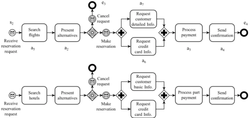
Consider a travel agency. Suppose that they have had in their infor-mation system two business process models named ‘flight-reservation’ and ‘hotel-reservation’, which correspond to flight and hotel booking functions (see Figure 2).
Receive reservation
request Search
ights alternativesPresent
Make reservation Cancel request Request customer detailed Info. Request credit card Info. Process
payment conrmationSend
s2 a5 a2 e3 a6 e4 a4 a3 a7 Receive reservation request Search hotels Present alternatives Make reservation Cancel request Request customer basic Info. Request credit card Info. Process part
payment conrmationSend
Figure 2: Flight & hotel reservation processes
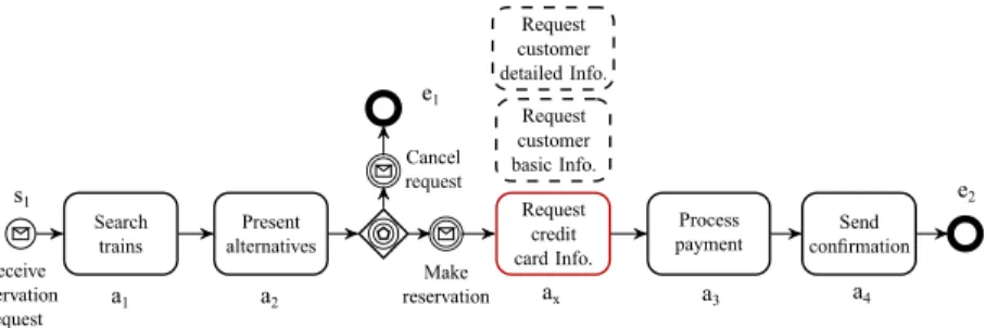
The travel agency decides to design a new process to offer a new train booking function. The process designer can rapidly sketch out the train-reservation process with some basic services as shown in Figure 3. Suppose that he is looking for a service, which is annotated by a round-corner rectangle with a ‘?’ symbol. This requested service has to fulfill some composition constraints, such as: it has to be executed before ‘Process payment’ and/or executed after ‘Present alternatives’ and/or has similar connection flows with the missing position, etc.
Existing approaches, such as text-matching mechanism and process equiv-alence, are not applicable for this inquiry as they do not provide a way to express composition constraints. Text-matching approaches do not consider
s1 a1 a2 e1 a4 e2 a3 ax ?
Figure 3: An incomplete train reservation process
the interactions between services in business processes.Whereas, process-querying approaches return similar process models instead of services. In this case, our approach can be applied as it focuses on the composition con-text around services. Concretely, it detects that the ‘unknown’ service has similar context with the ‘Request customer detailed Info.’, ‘Request customer basic Info.’ and ‘Request credit card Info.’ in the existing flight & hotel reser-vation processes (Figure 2) because they have similar connections from/to the same services, which are ‘Present alternatives’ and ‘Process payment’. So, we recommend these services for the missing position and the process designer may select the ‘Request credit card Info.’ service for this position as it is the most suitable (Figure 4).
s1 a1 a2 e1 a4 e2 a3 ax Request customer basic Info. Request customer detailed Info. Request credit card Info.
Figure 4: The complete train reservation process
We provide also a query language which allows the process designer to express his requests with flexible constraints (see details in section 5). By querying services based on composition context, our approach not only assists the process designer during the design time (completing a model or devel-oping new process variants) but also helps to guarantee the completion of business process instances during the execution time by finding alternatives of a service in case of failure.
3. Preliminaries
In this section, we present some notations and definitions that are used to formally define a business process (section3.1) and the composition context of a service (section3.2). We also explain how we handle loop cases (section3.3). We use the ‘train-reservation’ process (Figure 3) and the ‘flight-reservation’ process (Figure 2) to illustrate our approach.
3.1. Business Process Graph
As the structure of a business process can be mapped to a graph, we choose graph theory to present a business process. Indeed, there are a num-ber of graph-based business process modeling languages, e.g., BPMN, EPC, YAWL, and UML activity diagram. Despite their variances in expressiveness and modeling notations, they all share the common concepts of tasks, events, gateways, artifacts and resources, as well as relations between them, such as transition flows [39]. In our approach, we use BPMN in our approach to present business processes as it is one of the most popular business process modeling language.
We consider termination events (such as start or end events) as termi-nation services. We define a connection element as either a connecting ob-ject (e.g., sequence flow and message flow), or a gateway (e.g., AND-split, OR-split), or an intermediate event (e.g., error message, message-catching) (Figure 5). For example, in Figure 3, s1, a1, a2, e1 are services; and
‘flow-transition’, ‘event-based-gateway’ and ‘message-catching’ are connection el-ements. Although services and connection elements in our approach are defined using BPMN notations, they are easily mapped to equivalent nota-tions in other business process modeling and workflow languages, e.g., tasks and workflow control patterns [45].
: connection elements
Search
flights : services
Figure 5: Services and connection elements
Relations between services in a business process are presented by the execution orders between them. In our previous work [44], we considered only the causal relation between services, i.e., a service is situated next to another service (such as connection between a5 and a2 or a2 and a7 in Figure 2). In
parallel relations, i.e., the relations between services that belong to parallel flows, e.g. relation between a7 and a6 in Figure 2.
Let AP be the set of services and CP be the set of connection elements
in a business process P .
Definition 3.1 (next relation). Let ei, ej ∈ AP∪CP. A next relation ei to
ej, denoted by ei →P ej, indicates that ej follows ei in P .
Definition 3.2 (connected relation). Let ei, ej ∈ AP∪CP. ei is connected to
ej in P , denoted by ei ↔P ej, iff ei →P ej or ej →P ei.
Definition 3.3 (connection flow). A connection flow from ai to aj, ai, aj ∈
AP, denoted by aj
aifP, is a sequence of connection elements c1, c2, . . . , cn∈ CP
satisfying: ai ↔P c1, c1 ↔P c2, . . . , cn−1 ↔P cn, cn↔P aj. aj
aifP ∈ CP∗, CP∗ is
set of sequences of connection elements in P1.
Definition 3.4 (connected relation label). The label of a connected relation ei ↔P ej, ei, ej ∈ AP∪CP, denoted by l(ei ↔P ej), is defined as following:
l(ei ↔P ej) = eiej, if ei →P ej ejei, if ej →P ei
Definition 3.5 (connection flow label). The label of a connection flow ajaifP,
denoted by l(ajaifP), is defined as following:
l(ajaifP) = l(ai ↔P c1).l(c1 ↔P c2) . . . l(cn−1↔P cn).l(cn↔P aj)
where c1, c2, . . . , cn∈ CP: aj
aifP = c1c2. . .cn.
For example, the label of the connection flow from ‘Search flights’ to ‘Present alternatives’ in Figure2is: a5‘sequence’.‘sequence’a2; from ‘Present
alternatives’ to “Request customer detailed Info.” is: a2‘event-based-gateway’.
‘event-based-gateway’‘message-catching’.‘message-catching’‘parallel-split’. ‘parallel-split’a7.
We notice that:
1The connection flow from a
• An edge connecting two services ai, aj ∈ AP can be labeled by either
l(ajaifP) or l(aiajfP). For example, the edge connecting a5 to a2 in
Fig-ure 2 can be labeled by l(a2a5fP)=a5‘sequence’.‘sequence’a2 or l(a5a2fP)=
‘sequence’a2.a5‘sequence’.
• There can be more than one connection flow between two services. For instance, in the case that two services are connected by an AND-split and an AND-join (parallel relation). In this case, we number these connection flows to distinguish them. For example, there are two con-nection flows from a7 to a6 in Figure2and we number them as follows:
l(a6
a7fP1)=‘parallel-split’a7.‘parallel-split’a6 and l(a6a7fP2)=a7
‘synchroniza-tion’.a6‘synchronization’.
We consider each service as a node, each connection flow as an edge. We define business process as a multigraph, in which, set of edges is a multiset (Definition 3.6).
Definition 3.6 (Business Process graph). A business process graph of P is an undirected labeled multigraph GP = (VP, EP, LP, l) in which VP is a set of
nodes, EP is a multiset of edges, LP is a set of edge labels, and l is a mapping
function that maps edges to labels, where: • VP = AP,
• EP ⊆ hAP × AP, gi, g : AP × AP −→ N
g((ai, aj)) is the multiplicity of (ai, aj). If g((ai, aj)) > 1, the edges
connecting ai to aj are numbered by (ai, aj)t, t = 1..k, k > 1.
• LP = l(EP), where: l : EP −→ LP (ai, aj) 7→ l( aj aifP) , if g((ai, aj)) = 1 (ai, aj)t 7→ l( aj aifPt) , if g((ai, aj)) = k > 1, t = 1..k
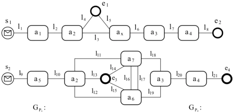
For example, the business process graphs of the ‘train-reservation’ process (Figure 3) and the ‘flight-reservation’ process (Figure 2) are presented in Figure 6.
a2 ax a3 a4 a1 s1 e1 e2 l1 l2 l3 l4 l5 l6 l7 l8 a5 a2 a7 a4 a3 a6 l9 l10 l11 l12 l13 l14 l15 l16 l18 l17 l20 l21 l19 s2 e3 e4 Edge labels: Annotation: S: ‘sequence’ E: ‘event-based-gateway’ M: ‘message-catching’ P: ‘parallel-split’ Y: ‘synchronization’ l8=‘‘a4S.Se4’’ l9=‘‘s2S.Sa5’’ l10=‘‘a5S.Sa2’’ l11=‘‘a2E.EM.MP.Pa7’’ l12=‘‘a2E.EM.MP.Pa6’’ l13=‘‘a2E.EM.Me3’’ l14=‘‘Me3.EM.EM.MP.Pa7’’ l15=‘‘Me3.EM.EM.MP.Pa6’’ l1=‘‘s1S.Sa1’’ l2=‘‘a1S.Sa2’’ l3=‘‘a2E.EM.Max’’ l4=‘‘a2E.EM.Me1’’ l5=‘‘Me1.EM.EM.Max’’ l6=‘‘axS.Sa3’’ l7=‘‘a3S.Sa4’’ G :P1
Edges: <(s1,a1),1>, <(a1,a2),1>, <(a2,ax),1>,
<(a2,e1),1>, <(e1,ax),1>, <(ax,a3),1>,
<(a3,a4),1>, <(a4,e2),1>
Nodes: s1, e1, e2, a1, a2, a3, a4, ax
G :P2
<(s2,a5),1>, <(a5,a2),1>, <(a2,a7),1>,
<(a2,a6),1>, <(a2,e3),1>, <(e3,a7),1>,
<(e3,a6),1>, <(a7,a6),2>, <(a7,a3),1>,
<(a6,a3),1>, <(a3,a4),1>, <(a4,e4),1>
s2, e3, e4, a2, a3, a4, a5, a6, a7
Edges: Nodes:
Figure 6: Business process graphs of the ‘train-reservation’ process (Figure 3) and the ‘flight-reservation’ process (Figure2)
3.2. Service Composition Context
We define the composition context of a service as a business process frag-ment that includes the associated service and the closest relations to its neighbors. A composition context is presented as a graph in which the as-sociated service is located at the center. Its neighbors are located in layers according to their shortest path lengths to the associated service. The com-position context of a service can be considered as a business fragment that presents the behavior of the associated service.
We present in the following some definitions that are used to formally define the composition context.
Definition 3.7 (connection path). A connection path from ai to aj in a
business process graph GP, denoted by aj
. . . , ak where a1 = ai, ak= aj and ∃(at+1at fP ∈ CP∗ ∨ atat+1fP ∈ CP∗) ∀1 ≤ t ≤
k − 1.
According to Definition3.7, a connection path in a business process graph is undirected. It means that the edges in a connection path can be oriented in different directions. For example, in Figure 2, a connection path from ‘Search flights’ (a5) to ‘Request customer detailed Info.’ (a7) can be either
‘a5, a2, a7’ or ‘a5, a2, a6, a7’ or ‘a5, a2, a6, a3, a7’, etc.
Definition 3.8 (connection path length). The length of a connection path
aj
aiPP, denoted by L( aj
aiPP) is the number of connection flows in the path.
Definition 3.9 (shortest connection path). The shortest connection path between ai and aj, denoted by
aj
aiSP, is the connection path between them that
has the minimum connection path length.
For example, in Figure 2, the shortest path from a5 to a7 is ‘a5, a2, a7’
and its length is 2.
Definition 3.10 (kth-layer neighbor). a
j is a kth-layer neighbor of ai in a
business process P iff ∃ajaiPP : L( aj
aiPP) = k. The set of kth-layer neighbors
of a service ai is denoted by NPk(ai). NP0(ai) = {ai}.
For example in Figure2, s2and a2 are the 1st-layer neighbors of a5; a5, e3,
a7 and a6 are the 1st-layer neighbors of a2; a6 is one of the 2nd-layer neighbors
of a5 and so on.
As the distance from a service ai to its kth-layer neighbors is k, we can
imagine that the kth-layer neighbors of a service ai are located on a circle
whose center is ai and k is the radius. The circle is latent since it exists but
it is not explicitly represented in the business process graph. We call this latent circle connection layer and the area limited by two adjacent latent circles connection zone. Connection layers and connection zones of a service are numbered. A connection flow connecting two (k − 1)th-layer neighbors,
or a (k − 1)th-layer neighbor to a kth-layer neighbor is called a kth-zone flow (Definition 3.11).
Definition 3.11 (kth-zone flow). av
aufP is a kth-zone flow of ai iff ∃avaufP :
(au, av ∈ NPk−1(ai)) ∨ (au ∈ NPk−1(ai) ∧ av ∈ NPk(ai)) ∨ (av ∈ NPk−1(ai) ∧ au ∈
NPk(ai)). The set of all kth-zone flows of a service ai ∈ P is denoted by
Zk
P(ai). ZP0(ai) = ∅ and |ZPk(ai)| is the number of connection flows in the kth
For example in Figure2, the connection from a2 to a7 is the 2nd-zone flow
of a5 while the connection from a7 to a3 is its 3rd-zone flow. |ZP22 (a5)| = 3 as
in the 2nd-zone of a5, there are three connection flows, which are from a2 to
a6, a7 and e3.
Intuitively, the connection paths between two services present their rela-tion in term of closeness. The longer the connecrela-tion path is, the weaker their relation is and the shortest connection path between two services presents their best relation. To illustrate the best relations of a service to others ser-vices in a business process, we define the service composition context graph (formally defined in Definition 3.12) which presents all the shortest paths from a service to others. Each service in a business process has a composition context graph. Each vertex in the composition context graph is associated to a number which indicates the shortest path length of the connection path to the associated service. The vertexes that have the same shortest path length value are considered to have the same distance to the associated service and are located on the same layer around the associated service. We name the number associated to each service in a composition context graph the layer number. The area limited between two adjacent layers is called zone. The edge connecting two vertexes in a composition context graph belongs to a zone. We assign to each edge in the composition context graph a number, so-called zone number, which determines the zone that the edge belongs to.
The edge connecting two services ai, aj in the composition context graph
of a service ax is associated to a zone number such that: if ai and aj are
located on two adjacent layers, the edge (ai, aj) will belongs to the zone
limited by the two adjacent layers; and if ai and aj are located on the same
layer, the edge connecting them belongs to the outer zone of the layer they are located on.
Concretely, assume that eij is the edge connecting two vertexes ai and aj
in the composition context graph of a service ax. The lengths of the shortest
connection paths connecting ai and aj to ax are l1 = L(axaiSP) and l2 = L( ax
ajSP) respectively. Let d = |l1− l2|, d has only two possible values, which are
0 and 1 (see our proofs [46], section A). In the case that d = 0 (l1 = l2), i.e.,
ai and aj are both l1th-layer neighbors of ax, we assign to eij l1 + 1 as zone
value. In the case that d = 1, i.e., ai and aj belong to two adjacent layers,
eij is the kth-zone flow connecting ai and aj and we assign to eij the zone
value k, i.e., min(l1, l2) + 1. Consequently, we assign to the connection flow
connecting ai and aj in the composition context graph of ax the value M in(
L(ax
the context graph of ax will be M ax(L(axatSP)) + 1 ∀at∈ P .
In any linked business process graph, we can always calculate the shortest path length between two services. Therefore, in the composition context graph of a service, we can always identify the layers on which services are located. Consequently, we can always assign layer number to a service and thus, zone number, to a connection flow in a composition context graph.
Gax P1 ax a2 a3 a1 a4 1s tla ye r 2ndla ye r 3rdla ye r 1s tzone 2ndzone 3rdzone l1 l2 l4 l5 l3 l6 l 7 s1 e1 e2 l8 Ga6 P2 a6 a2 a3 a7 a4 1s tla ye r 2ndla ye r 3 rdla ye r 1s tzone 2ndzone 3rdzone a5 l19 l9 l10 l12 l11 l13 l14 l15 l16 s2 e3 e4 l18 l20 l17 l21 Edge labels: Annotation: S: ‘sequence’ E: ‘event-based-gateway’ M: ‘message-catching’ P: ‘parallel-split’ Y: ‘synchronization’ l16=‘‘Pa7.Pa6’’
l17=‘‘a7Y.a6Y’’
l18=‘‘a7Y.Ya3’’ l19=‘‘a6Y.Ya3’’ l20=‘‘a3S.Sa4’’ l21=‘‘a54S.Se4’’ l8=‘‘a4S.Se4’’ l9=‘‘s2S.Sa5’’ l10=‘‘a5S.Sa2’’ l11=‘‘a2E.EM.MP.Pa7’’ l12=‘‘a2E.EM.MP.Pa6’’ l13=‘‘a2E.EM.Me3’’ l14=‘‘Me3.EM.EM.MP.Pa7’’ l15=‘‘Me3.EM.EM.MP.Pa6’’ l1=‘‘s1S.Sa1’’ l2=‘‘a1S.Sa2’’ l3=‘‘a2E.EM.Max’’ l4=‘‘a2E.EM.Me1’’ l5=‘‘Me1.EM.EM.Max’’ l6=‘‘axS.Sa3’’ l7=‘‘a3S.Sa4’’
Figure 7: Composition context graphs of ax(in Figure 3) and a6(in Figure 2)
Definition 3.12 (Composition context graph). The composition context graph of a service ax ∈ P , denoted by GaxP = (V
ax
P , E
ax
P , LP, l), is an
undi-rected labeled multigraph created from GP = (VP, EP, LP, l). VPax is a set of
vertexes associated to their layer numbers and EPax is a set of edges associated to their zone numbers. VPax and EPax are defined as following:
- EPax = {(< (ai, aj), g((ai, aj)) >, aj
aizaxP ) :< (ai, aj), g((ai, aj)) >∈ EP, aj
aizaxP = M in(L(axaiSP), L(axajSP)) + 1}
For example, the composition context graphs of the ‘unknown’ service (ax in Figure 3) and the ‘Request credit card Info.’ (a6 in Figure 2) are
presented in Figure 7. In these graphs, all causal and parallel flow relations are presented.
3.3. Loop Cases
There are three typical loop cases in a business process: self-loop, loop via another service and loop via other services. By applying Definition 3.12, the possible layers to which the loop services can belong are depicted in Figure8.
kth-zone (k+1)th-zone
(k+1)th-layer kth-layer
(k-1)th-layer ai
(a) Self loop
kth-zone (k+1)th-zone (k+1)th-layer kth-layer (k-1)th-layer aj ai ah
(b) Loop via another service
kth-zone (k+1)th-zone (k+1)th-layer kth-layer (k-1)th-layer aj ai ah
(c) Loop via other services Figure 8: Connection flows in loop cases
In the self-loop case (Figure8a), if a service ai is located on the kth-layer,
then its self-loop edge belong to the zone (k + 1)thbecause according to
Defi-nition3.12, the zone number of this edge isai
aiz
ax
P = M in(L(aiaxSP), L(aiaxSP))+
1 = M in(k, k) + 1 = k + 1.
In the loop-via-another-service case (Figure 8b), there are two possibili-ties: (i) the two services are located on adjacent layers (e.g., aj and ai) and
(ii) the two services are located on the same layer (e.g., ai and ah). In the first
possibility, assume that ai and aj are respectively located on the (k − 1)th
-layer and kth-layer, the edges connecting them are assigned the zone number aj aizPax =aiaj z ax P = M in(L( ai axSP), L( aj axSP)) + 1 = M in(k − 1, k) + 1 = k,
i.e., they are on the zone limited by these adjacent layers. In the sec-ond possibility, assume that ai and ah are located on the same kth-layer,
the edges connecting them are assigned the zone number ahaizaxP =aiah zaxP = M in(L(ai
axSP), L(ahaxSP)) + 1 = M in(k, k) + 1 = k + 1, i.e., they are presented
In the loop-via-other-services case (for example, Figure8cshows the loop created by 3 services), the edges between services are assigned their zone numbers following Definition 3.12. For the two services located on adjacent layers (e.g., aj and ai, or aj and ah in Figure 8c), the edge connecting them
belongs to the zone limited by these layers. For the two services located on the same layer (e.g., ai and ah in Figure 8c), the edge connecting them
belongs to the outer zone of their layer.
So, in any business process graph, including graphs that contain loops, we can always calculate the shortest path length between two services. There-fore, in the composition context graph of a service, we can always identify the layers on which rest services are located. Consequently, we can always assign a layer number to a service and thus, a zone number to a connection flow, in a composition context graph.
4. Composition Context Similarity
The kth-zone neighbors of a service and their connection flows create a
process fragment around the associated service. This fragment contains the business context that reflects the behavior of the associated service. In this section, we present our methodology to compute the matching between two composition contexts. We firstly present how we match two connection flows (section 4.1). Then, we elaborate the matching between two composition contexts (section 4.2). Finally, we show how we integrate the similarity between connection elements into our composition context similarity compu-tation (section 4.4).
To illustrate the computation process, we will consider the composition context of the ‘unknown’ service in the ‘train-reservation’ process (ax in
Fig-ure 3) and the ‘Request credit card Info.’ service in the ‘flight-reservation’ process (a6 in Figure 2). The composition context graphs of these services
are shown in Figure 7.
4.1. Connection Flow Matching
To compute the matching between two connection flows, we propose to use the Levenshtein distance (LD for short) [47]. In information theory, the LD is a metric for measuring the difference between two sequences of characters. The LD is defined as the minimum number of edits needed to transform one sequence of characters into the other, with the allowable edit operations being insertion, deletion, or substitution of a single element. For
example, the LD between “gumbo” and “gambol” is 2, between “kitten” and “sitting” is 3, etc. Inspired by this, we consider each connection element in a connection flow as a character and we label connection flows as a sequence of characters. Then, the similarity between two connection flows can be computed based on the similarity of their labels using LD.
Let st1 = l(avaufP1), st2 = l(anamfP2). Let Dif f be a function that computes
the difference between two connection flows. We have:
M (avaufP1,anamfP2) = 1 − Dif f (st1, st2) M ax(length(st1), length(st2)) (1) where: • Dif f (st1, st2) = LD(l(avaufP1), l(amanfP2)), if (au = am) ∧ (av = an) • Dif f (st1, st2) = LD(l(avaufP1), l(anamfP2)), if (au = an) ∧ (av = am)
• Dif f (st1, st2) = M ax(length(st1), length(st2)), i.e., M (avaufP1,anamfP2) =
0, in other cases.
For example in Figure7, we have Mp(a4a3fP1,a3a4fP2) = M (“a3S.Sa4”, “a3S.Sa4”)
= 1 − 04 = 1; Mp(a2a1fP1,a2a5fP2) = 0 and so on.
We prove that LD of two strings is equal to LD of their inverse strings (see our proofs [46], section B). So, whatever the edges (au, av) and (am, an)
are labeled by l(avaufP1) or l(auavfP1) and l(anamfP2) or l(amanfP2), Equation 1 gives
the same value.
In the case that there is more than one connection flow between two services, we compute all possible matching between them and we select the best matching value.
4.2. Composition Context Matching
To compute the composition context matching between two services, we propose to sum up the matching of the connection flows in the two contexts. There are two cases to consider: the first zone and other zones. In the first zone, we match the connection flows that connect the two associated services and same services in the first layer. In other zones, we match the connection flows that connect the same services. We sum all matching values then divide them by the number of connection flows in the considered zones of the first service.
We apply Equation 1 to compute the composition context matching in either the first and other zones. However, Equation1 considers only connec-tion flows that connecting the same services in two business processes. So, to adapt it in the first zone, we assume that the two associated services have the same name, so-called a0. Then, we match connection flows connecting
a0 to the same services in the first layer.
Formally, let ai, aj are two associated services. We change ai, aj to a0.
Then, ∀ac∈ NP11 (ai) ∩ NP21 (aj), we compute the similarity betweenacaifP1 and ac
ajfP2 based on the similarity between aca0fP1 and aca0fP2.
Basically, the composition context matching between ai ∈ P1 and aj ∈ P2
within k zones, denoted by MCk(GaiP1, GajP2), is computed by Equation2.
MCk(GaiP1, G aj P2) = k X t=1 X av aufP1∈ZP1t , an amfP2∈ZP2t MFt(avaufP1,anamfP2) k X t=1 |ZP1t (ai)| (2)
where k is the number of considered zones, |Zt
P1(ai)| is the number of
con-nection flows in the tth zone of GaiP1, and MFt(auavfP1,anamfP2) is the matching
value of av aufP1 and anamfP2 in zone t: MFt(avaufP1,anamfP2) = M (avaufP1,anamfP2) if t = 1, (au = am) ∨ (av = an) ∨(au = av ∧ am = an) t 6= 1, (au = am∧ av = an) 0 other cases
For example, the composition context matching between ax and a6
(Fig-ure 7) computed by Equation 2 is:
MC3(GaxP1, G a6 P2) = M (axa2fP1,a6a2fP2) + M (axe1fP1,a6e3 fP2) + M (a3axfP1,a3a6fP2) +M (e1a2fP1,e3a2fP2) + M (a4a3fP1,a4a3fP2) + M (e2a4fP1,e4a4fP2) 3 + 3 + 2 = 3 4 + 4 5 + 1 2 + 1 + 1 + 1 8 = 0.63
4.3. Zone Weight
The behavior of a service is strongly reflected by the connection flows to its closet neighbors while the interactions with other neighbors in the further layers do not heavily reflect its behavior. Therefore, we propose to assign a weight (wt) for each tth connection zone, so called zone-weight and integrate
this weight into the similarity computation. Since the zone-weight has to have greater values in smaller tth connection zone, we propose a zone-weight value computed by a polynomial function which is wt=
k + 1 − t
k , where t is the zone number (1 ≤ t ≤ k) and k is the number of considered zones around the service. All connection flows connecting the associated service have the greatest weight (w1 = 1) and the connection flows connecting services in the
furthest zone have the smallest weight (wk = 1k).
Then, the composition context matching between GaiP1 and GajP2 within k zones and with zone weight, denoted by MWk(GaiP1, GajP2), is given by Equa-tion 3. MWk(GaiP1, G aj P2) = 2 k + 1× k X t=1 k + 1 − t k × X av aufP1∈ZP1t an amfP2∈ZtP2 MFt(avaufP1,anamfP2) |Zt P1(ai)| (3) where: MFt(avaufP1,anamfP2) = M (av aufP1,anamfP2) if t = 1, (au = am) ∨ (av = an) ∨(au = av ∧ am = an) t 6= 1, (au = am∧ av = an) 0 other cases
For example, the composition context matching between ax and a6
(Fig-ure 7) computed by Equation 3 is:
MW3(GaxP1, G a6 P2) = 2 3 + 1 × ( 3 3 × M (ax a2fP1,a6a2fP2) + M (axe1fP1,a6e3 fP2) + M (a3axfP1,a3a6fP2) 3 + 2 3× M (e1 a2fP1,e3a2fP2) + M (a4a3fP1,a4a3fP2) 3 + 1 3 × M (e2 a4fP1,e4a4fP2) 2 ) = 2 4× ( 3 3 × 3 4 + 4 5 + 1 2 3 + 2 3× 1 + 1 3 + 1 3 × 1 2) = 0.65
4.4. Similarity Between Connection Elements
Connection elements serve as fundamental factors to specify execution constraints and dependencies between services. For example, a sequence specifies a causal relation, an AND-split specifies a parallel execution, an OR-split specifies a choice, etc. The connection elements can show common execution behavior such as sequential, concurrent, choice, etc. So, their behaviors are not totally different. For example, consider two services ai and
aj that can be connected by: (1) a ‘sequence’ or (2) an ‘AND-split’. The
two connection elements are different, however, they have common execution behavior, which is: aj is executed right after ai.
In the previous sections (4.2 and 4.3), we consider that the matching between two connection elements has only two values: 0 (in the case that they do not have the same type) and 1 (in the case that they have the same type). In this section, we propose a metric to compute the similarity between connection elements in terms of execution properties. This metric allows evaluating their similarity by a real value between 0 and 1.
We firstly identify matching rules that the similarity has to satisfy
(sec-tion 4.4.1). Then, we present our proposition to compute the similarity
be-tween typical connection elements (section 4.4.2). Finally, we describe how to integrate the computed similarity into the composition context matching (section 4.4.3).
4.4.1. Matching Rules
In our work, we deal with basic connection elements, which are sequence, AND, OR and XOR as they are commonly used in business processes. Other elements and complex gateways are not considered. However, the same prin-ciples and methodology can be applied.
We present our analysis on the ‘-split’ elements, including AND-split, OR-split and XOR-split. A ‘-split’ connection element consists of one input and multiple output flows. The similarities between ‘-join’ elements can be inferred with the same reasoning.
To compute the similarity between connection elements, we firstly specify three matching rules that our approach satisfies, which are:
¬ If two connection elements are identical, their similarity is 1.
For example, similarity of two ‘sequence’ is 1; similarity of two ‘AND-split’ elements is 1 and so on.
Similarity between two connection elements that have the same types but different number of output flows is 1. Similarity between two dif-ferent connection elements is less than 1.
For example, similarity between two ‘AND-split’ elements that have different number of output flows is 1 whereas similarity between an ‘AND-split’ and an ‘OR-split’ is less than 1.
® In the case that two connection elements are different, the less different the numbers of output flows are, the greater similarity value is.
For example, consider the matching between an ‘AND-split’ that has 2 output flows and two ‘OR-split’ that have respectively (1) 2 output flows and (2) 3 output flows. The similarity value of the ‘AND-split’ and the first ‘OR-split’ must be higher than the similarity value of the ‘AND-split’ and the second ‘OR-split’.
4.4.2. Similarity Computation
Connection elements indicate the number of possible execution cases. The number of possible execution cases is impacted by the type of the connection element and the number of output flows derived by the connection element. In our approach, we analyze the number of possible execution cases and compute the similarity between connection elements based on the probability that an output flow is executed.
Consider the case where two services ai and aj are connected by a
con-nection element c. The concon-nection flow from ai to aj is notated by aj aif = c.
c can be a sequence, an ‘AND-split’, an ‘OR-split’ or an ‘XOR-split’.
We call a case that satisfies the constraints of a connection element a ‘possible execution case’ or a ‘possible case’ in short. For example, if c is a ‘sequence’, it has only one possible execution case, in which the service following c is executed; if c is an ‘AND-split’, it also has one possible execution case in which all services pointed by the output flows of c are executed; but if c is an ‘OR-split’, it has multiple execution cases: ‘at least one of the services pointed by output flows needs to be executed’.
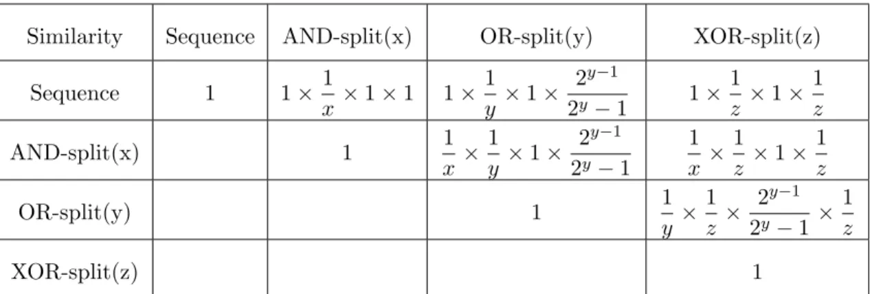
Let x, y and z be the number of output flows that an ‘AND-split’, an ‘OR-split’ and an ‘XOR-split’ respectively have. The numbers of possible cases of these connection elements are given in the 4th column of Table 1.
The last column of Table 1 presents the probabilities that an output flow is executed. We explain in the following how we compute these values.
For the ‘sequence’ and ‘AND-split’ cases, there is only one possible exe-cution case, in which all services are executed. Hence, the probability that
Element Presentation No. paths No. pos-sible cases
Probability that an output flow is exe-cuted Sequence ai aj 1 1 1 AND-split ai aj 1 x x 1 1 OR-split ai aj y 1 y 2y − 1 2 y−1 2y− 1 XOR-split ai aj z 1 z z 1 z
Table 1: Probability that aj appears in the possible cases
an output flow is executed is 1.
For the ‘OR-split’ case, the execution is completed if at least one of y services in the y output flows is executed. The number of cases where at least one of y services is executed is 2y− 1. On the other hand, the number of possible cases where an output flow is ‘executed’ is 22y = 2y−1. So, the
probability that an output flow is executed is 22yy−1−1.
For the ‘XOR-split’ case, for z output flows, there are z possible execution cases. Therefore, the probability that an output flow is executed is 1z.
To compute the similarity between these connection elements, we pro-pose to combine the weight of an output flow and the probability that it is executed. The weight of an output flow is specified by the inverse number of output flows. For example, consider an ‘AND-split’ that derives 3 output flows. The weight of each output flow is 13.
Consequently, the similarity between two connection elements cu and cv,
denoted by S(cu, cv), is given as following:
S(cu, cv) = w∗cu× w ∗ cv × P + cu × P + cv (4)
where w∗(cu), w∗(cv) are respectively weights of an output flow of cu and cv;
P+
cu and Pcv+ are probabilities that an output flow of cu and cv is executed.
The similarities between aforementioned connection elements are given in Table 2. In the section C of our proofs [46], we prove that the similarities computed by our approach satisfy the aforementioned matching rules.
Similarity Sequence AND-split(x) OR-split(y) XOR-split(z) Sequence 1 1 ×1 x × 1 × 1 1 × 1 y × 1 × 2y−1 2y− 1 1 × 1 z× 1 × 1 z AND-split(x) 1 1 x× 1 y × 1 × 2y−1 2y− 1 1 x × 1 z × 1 × 1 z OR-split(y) 1 1 y × 1 z × 2y−1 2y− 1× 1 z XOR-split(z) 1
Table 2: Similarities between typical connection elements
For example, with x = 2, y = 3, z = 4, S(AND-split,sequence)=0.5, S(OR-split,sequence)=0.19, S(XOR-split,sequence)=0.06, S(AND-split,OR-split)=0.10, S(AND-split,XOR-split)=0.03 and S(OR-split,XOR-split)=0.01.
4.4.3. Integration into the Composition Context Matching
The composition context matching is computed from the matching of connection flows (section 4). A connection flow is a sequence of connection elements that connect two services (Definition 3.3). It can contain one or more connection elements. We propose to integrate the similarity between connection elements in the case where connection flows contain only one con-nection element. For example, consider two concon-nection flowsayaxfP1 and avaufP2
of two composition context graph GaiP1 and GajP2. Assume that they are located on the same connection zone and connect the same ending services. Each of them contains only one connection element, which is c and c0 respectively. Similarity between them is inferred by the similarity between the connection elements, which is computed by Equation 4.
In the case that connection flows contain more than one connection el-ement, we transform them to strings of characters and reuse Levenshtein distance to compute their similarity (section 4.1).
As the similarity between connection elements is applied to compute the similarity of connection flows, it impacts on the final result of the composition context matching. In our experiments, we analyze matching cases with and without the similarity between connection elements to assess its impact.
5. Service Querying
Each service in a business process has a composition context which presents the relations between the service and its neighbors. By matching composi-tion contexts, we can find services that have similar relacomposi-tions to common neighbors. In this section, we present a query language used to retrieve rel-evant services to a selected position in a business process (section 5.1) and its execution (section 5.2).
5.1. Query Grammar
The query in our approach not only helps to search for relevant services based on a given composition context but also allows adding constraints to filter the searching results. It consists of three parameters, which are: an associated service, connection constraints, and a radius. The associated service is the service whose composition context is considered to be matched with other contexts. Connection constrains are services or connection flows to be included/excluded to filter the query’s results. The radius is the number of connection layers taken into account for the composition context matching. It specifies the largeness of the considered composition contexts.
We present in the following our proposed query grammar using the Ex-tended Backus-Naur Form (EBNF)2 [48]. We use ‘;’ to separate the input
parameters; ‘(’ and ‘)’ to separate query’s constrains; ‘<’ and ‘>’ to group services or connection flows; ‘[’ and ‘]’ to separate a connection flow and its ending services. We use ‘+’ and ‘-’ signs to include/exclude constraints; and ‘|’ sign for multiple choice operator. Details of the grammar are presented in Table 3.
1. Query ::= ServiceID,‘:’,[Constraint],‘:’,Radius; 2. ServiceID ::= Character,{Character|Digit}; 3. Constraint ::= (‘+’|‘-’)Term | Constraint,‘|’,Term; 4. Term ::= Item | Term,‘+’,Item | Term,‘-’,Item; 5. Item ::= ServiceID| ConFlow | ‘(’,Constraint,‘)’;
6. ConFlow ::= ‘<’,[ServiceID],‘[’,FlowString,‘]’,[ServiceID]‘>’;
7. FlowString ::= ConElement,{ConElement};
8. ConElement ::= ‘sequence’|‘AND-split’|‘AND-join’|‘OR-split’|‘OR-join’|‘XOR-split’|‘XOR-join’;
9. Radius ::= DigitNotZero,{Digit};
10. Character ::= ‘a’ | ‘b’ | ‘c’ | ‘d’ | ‘e’ | ‘f’ | ‘g’ | ‘h’ | ‘i’ | ‘j’ | ‘k’ | ‘l’ | ‘m’ | ‘n’ | ‘o’ | ‘p’ | ‘q’ | ‘r’ | ‘s’ | ‘t’ | ‘u’ | ‘v’ | ‘w’ | ‘x’ | ‘y’ | ‘z’;
11. DigitNotZero ::= ‘1’ | ‘2’ | ‘3’ | ‘4’ | ‘5’ | ‘6’ | ‘7’ | ‘8’ | ‘9’; 12. Digit ::= ‘0’ | DigitNotZero;
Table 3: Query grammar The query grammar is explained as follows:
• The query is defined in line 1 with three parameters separated by ‘:’. The constraint is optional. It can be defined to filter the query result. It can also be absent if we want to execute only the composition context matching without filtering.
• In line 2, the service identifier is defined as a string of characters or digits. It has to start by a character.
• In line 3, we define constraints. A constraint can be an included/excluded service or a connection flow. It can also include different items and op-erators. Operators in a constraint can be OR, INCLUDE, EXCLUDE. We use ‘|’, ’+’ and ‘-’ to specify these operators. Consequently, we define a constraint as a ‘Term’ or another constraint with ‘|’ operator. • In line 4 we define a ‘Term’ as an ‘Item’ or another constraint with the
‘+’ and ‘-’ operators.
• The ‘Item’ is defined in line 5. It can be a service or a connection flow that is included/excluded in the query. It can also be another constraint which is grouped by ‘(’ and ‘)’. Definitions in line 3, 4 and 5 allow specifying a constraint with multiple services, connection flows, operations and grouped conditions.
• In line 6, we define a connection flow which is presented within ‘<’ and ‘>’ signs. It includes a string of connection elements connecting two
services.
• The string of connection elements is defined in line 7. It includes at least a connection element which is defined in line 8.
• In line 9, we define the radius as a natural number greater than 0. • Finally, lines 10, 11, 12 define literal characters and digits.
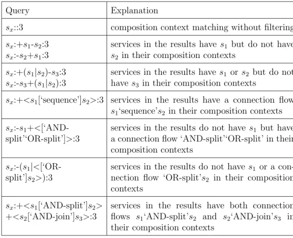
Examples of our query are given in Table4. These queries are used to find services that have composition contexts similar to the composition context of sx. These composition contexts are limited to 3 layers. In Table4, we also
explain the concerned constraints used to filter the query result.
Query Explanation
sx::3 composition context matching without filtering
sx:+s1-s2:3
sx:-s2+s1:3
services in the results have s1 but do not have
s2 in their composition contexts
sx:+(s1|s2)-s3:3
sx:-s3+(s1|s2):3
services in the results have s1 or s2 but do not
have s3 in their composition contexts
sx:+<s1[‘sequence’]s2>:3 services in the results have a connection flow
s1‘sequence’s2 in their composition contexts
sx:-s1
+<[‘AND-split’‘OR-split’]>:3
services in the results do not have s1 but have
a connection flow ‘AND-split’‘OR-split’ in their composition contexts
sx:-(s1
|<[‘OR-split’]s2>):3
services in the results do not have s1 or a
con-nection flow ‘OR-split’s2 in their composition
contexts sx:+<s1[‘AND-split’]s2>
+<s2[‘AND-join’]s3>:3
services in the results have both connection flows s1‘AND-split’s2 and s2‘AND-join’s3 in
their composition contexts
Table 4: Query examples
In our motivating example (Figure 3), as the designer wants to find ser-vices whose composition contexts are similar to ax, he selects ax as the
the queried service should be executed right after ‘Present alternatives’ (a2)
and before ‘Process payment’ (a3) and (2) it is connected from a2 by a
connection flow ‘event-based-gateway’‘message-catching’ and to a3 by a
‘se-quence’. Finally, he specifies the radius, which is 1 in this case, because he wants to find the contexts in which a2 and a3 are connected directly
to ax. Consequently, his query is: ax:+<a2
[‘event-based-gateway’‘message-catching’]>+<[sequence]a3>:1.
More examples about our query can be given as follows. If the process designer wants to find services that have similar context to ‘Search trains’ (a1) within the first zone, he can make a query as following: a1::1. If he
wants to find services that are similar to ‘Search trains’ but not followed by ‘Present alternatives’, he will exclude the connection flow connecting ‘Search trains’ to ‘Present alternatives’ in its first layer. The query will be: a1
:-(<a1[sequence]a2>):1. In the case that he wants to know possible payment
methods, he may select ‘Process payment’ service (a3) and add a constraint
which does not include a ‘sequence’ that connects to ‘Send confirmation’ service (a4). He can also widen the considered composition context in two
layers to get more results. So, his query is: a3:-(<[‘sequence’]a4>):2. Or, if he
wants to find services that are similar to ‘Search trains’ (a1), and include the
services ‘Request payment Info.’ (a8) and ‘Process payment’ (a3) but exclude
the AND-join connection between them, his query is as follows: a1:+a8+a3
-(<a8[‘AND-join’]a3>):5, etc.
5.2. Query Execution
In general, queries are processed as follows:
1. We capture the composition context of the associated service. The largeness of the composition context is specified by the radius param-eter.
2. We match the composition context of the associated service to compo-sition contexts of other services in other processes.
3. We refine the matching result by selecting only services whose compo-sition contexts satisfy the query’s constraints.
4. We sort the selected services based on the matching values and pick up top-N services3 for the response.
6. Implementation & Experiments
In this section, we present our implementation (section 6.1) and experi-ments (section 6.2) to validate our approach.
6.1. Implementation
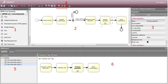
To demonstrate our approach, we implemented an application that allows the process designer to create business processes and get recommendations during the design phase. Our application was developed based on Signavio4,
which is a platform for business process design. This platform provides a web-based graphical interface to design business processes. It uses BPMN notations. It has two versions: commercial and open source. The open source version with limited features is published5 for free downloading and testing. By developing our approach based on Signavio, we achieve two targets: (1) we propose a user-friendly tool through the graphical suite and (2) we widen the user community and make our approach visible as Signavio is widely known in the community. Our tool is published at http://www-inf.
it-sudparis.eu/SIMBAD/tools/WebRec/.
Figure 9: Application screen-shot
4http://www.signavio.com/
In this application, the process designer can design and store business processes. During the design, he can select a service and process a query. He needs to specify the number of layers/zones needed to be taken into account and choose an algorithm to be executed. The composition context matching is executed beforehand. Then, query constraints are applied on the matching result to filter unrelated services. Queries and their results can be saved and reloaded for a future use.
A screen-shot of the application is shown in Figure9. The areas 1, 2 and 3 show the BPMN elements for design, canvas and property of the selected element. They are provided by the Signavio platform. We developed the areas 4, 5, and 6. Area 4 contains the buttons for launching the context matching and query, area 5 shows the list of previous queries and area 6 displays either the query design or its results.
A basic scenario6 is as follows:
1. A process designer opens the application to design a new process. He can also load an existing process for editing.
2. During the design, he can select a service, create a query, and specify the number of layers (or zones) needed to be taken into account for the composition context matching.
3. He can select to run one of 4 prepared algorithms7.
4. The application executes the query and returns results. When the designer selects a service from the result, it shows the corresponding process in which the selected service is highlighted.
5. The designer can copy services from the returned process and paste them on the active canvas to continue his design.
6. He can save the executed query for future usage. He can also load, modify and executed a saved query.
6.2. Experiments
We performed experiments on a large public collection of business pro-cesses. Our goal is three fold: (i) to evaluate the feasibility of our approach;
6Tutorial at:
http://www-inf.it-sudparis.eu/SIMBAD/tools/WebRec/tutorial. html and video demo at: http://www-inf.it-sudparis.eu/SIMBAD/tools/WebRec/ demo.html
7at the current stage, we have developed 4 algorithms for the composition context
matching, which are with/without zone weight and with/without connection element sim-ilarity
(ii) to measure its accuracy and to (iii) evaluate the performance of our algorithm. Details of the dataset and experiments are given as following. 6.2.1. Dataset & Experimental Cases
The dataset used in our approach is shared by the Business Integration Technologies (BIT) research group8 of the IBM Zurich [49]. It contains
busi-ness process models designed for financial services, telecommunications, and other domains. It is presented in XML format following BPMN 2.0 standard. Each XML file stores the data of a business process, including elements’ IDs, service names, and the sequence flows between elements. The dataset con-sists of 560 business processes with 6363 services. There are 3781 different services in which 1196 services appear in more than one process. In average, there are 11.36 services, 18.96 gateways (including parallel, exclusive and inclusive gateways) and 46.81 sequence flows in a process.
We performed experiments to measure the feasibility, the accuracy and the performance of our approach. We evaluate the feasibility based on the number of services whose matching values with others are greater than a given threshold. We also observe the impact of the number of selected zones (kth-zone number) and zone weight on the number of returned services. We
evaluate the accuracy based on the Precision and Recall and we evaluate the performance based on the computation time.
Our algorithm was experimented with 5 different cases which are pre-sented in Table 5. In Case 1, we considered only the zone-weight. The parallel flow relations and connection element similarity were not taken into account in the composition context matching. In Case 2, we considered only the parallel relations, regardless the zone-weight and connection element sim-ilarity. Case 3 took into account both parallel flow relations and zone-weight, whereas Case 4 considered parallel relations and connection element similar-ity. In Case 5, the algorithm was performed with all parameters above.
In our previous work [44], we presented some preliminary results of the first case, which considers only zone weight and consecutive relations between services. In this work, apart from the additional results of the first case, we present and discuss about the experimental results of the other cases which take into account parallel relations between services and similarity between connection elements.
Case 1 Case 2 Case 3 Case 4 Case 5
Parallel flow relations x x x x
Zone-weight x x x
Connection element similarity x x
Table 5: Examined cases
6.2.2. Results
- Approach feasibility and parameter impact :
In the first experiment, we aim at evaluating the feasibility of the ap-proach and the impact of parameters. The feasibility is evaluated based on the number of services that can have recommendations. Figure10shows the percentages of services whose matching values with other services are greater than or equal to 0.5. It shows that cases 2, 3, 4, 5, which take into account the parallel flow relations, retrieve greater number of services than case 1. The zone-weight parameter has no impact in the first zone. Hence, with k = 1, case 2 and case 3 has the same number of services (similar to case 4 and 5). However, with k = 2, the number of services and similarity values decreased. Case 3 and case 5, which take into account zone weight in their computation, retrieve more services than case 2 and case 4 respectively. It means that zone weight impacts on the number of retrieved services. When we take into account zone weight, we retrieve more services. Similarly, the similarity between connection elements impacts on the number of retrieved services. When we take into account similarity between connection elements (case 4 and case 5 compared to case 2 and case 3 respectively), we retrieve more services. Case 5, which takes into account both zone-weight and con-nection element similarity, retrieves the highest number of services.
In this experiment, we obtained 77.7% services whose matching values are greater than 0 and 21.48% services whose matching values are greater than 0.5. In the worst cases, we obtained 61.3% services whose matching values are greater than 0 and 8.57% services whose matching values are greater than 0.5. These results show that our approach can provide recommendations for a majority services as we can retrieve similar services for more than 2/3 number of services in average. It means that our approach is feasible and can be applied in real use-cases.
0 0.05 0.1 0.15 0.2 0.25 k=1 k=2 Percen ta ge o f servi ces kth-‐zone number Case 1 Case 2 Case 3 Case 4 Case 5
Figure 10: Percentage of services whose matching value >= 0.5
To examine the impact of kth-zone values, we run our algorithms with k from 5 to 1. The experimental results (Figure 11) show that when k decreases, the number of recommended services increases. It is because when k decreases that the number of unmatched services in further layers decreases, the matching values between composition contexts increase, the number of services increases.
This experimental results also show that zone-weight and similarity be-tween services impact on the number of retrieved services. Cases 3 and case 5, which take into account zone-weight, has more services than case 2 and 4 respectively. Similarly, cases 4 and 5, which take into account similarity between services, has more services than case 2 and 3 respectively.
0 0.05 0.1 0.15 0.2 0.25 k=5 k=4 k=3 k=2 k=1 Per ce n tage o f ser vi ce s kth‐zone number Case 1 Case 2 Case 3 Case 4 Case 5
Figure 11 also shows the impact of parallel flow relations. When we take into account the parallel flow relations between services, many services located on the further layers of a composition context graph are relocated on the nearer layers. Therefore, the matching values in the first zone are high and these values decrease quickly when we consider further zones. Figure 11
shows that in Cases 2, 3, 4 and 5, which take into account parallel flow relations, the number of services is very low with great k and very high with small k. Meanwhile, in Case 1, the number of services slightly change when k decreases.
- Algorithms accuracy :
Our approach is based on service composition context regardless the iden-tifier of the considered service. The ideniden-tifier of a service is used just for determining the associated composition context. In this experiment, we aim at using it as the ground-truth data for the Precision and Recall computa-tion. Our objective in to assess how accurate is our approach when it is used to recommend services for an empty position in a process. To do so, for a selected service in a process, we consider this service as an unknown service. We compute recommendations for this selected position. A relevant recommendation should contain the selected service.
Concretely, consider a selected service s in a process P . Assume that s appears in n processes. The recommendations for this selected position consist of l services, in which t(t ≤ l) services are s. Precision and Recall of these recommendations are given by Equation 5.
P recision = t
l; Recall = t
n (5)
In our experiment, we tune the number of recommended services for each position from 5 to 1. We consider the matching in the first zone. To ignore the noise of the irrelevant processes, we compute Precision and Recall for only the services that appear in at least 10 business processes. Consequently, 29 services and 267 processes are used in our experiment.
The average Precision and Recall values are shown in Figure 12. The Precision and Recall values of the examined cases are not so different, as the different parameters that distinguish these cases has a slight impact if we consider just the the first zone (as explained in the previous section). The Precision values increase when the number of recommended services de-creases. This means that the relevant services mostly appear at the top of the recommendation list. In other words, when we shorten the recommendation
0.4 0.45 0.5 0.55 0.6 0.65 0.7 0.75 0.8 0.85 5 4 3 2 1 Preci si on
Number of recommended services
Case 1 Case 2 Case 3 Case 4 Case 5 0 0.02 0.04 0.06 0.08 0.1 0.12 0.14 5 4 3 2 1 Re ca ll
Number of recommended services
Case 1 Case 2 Case 3 Case 4 Case 5
Figure 12: Precision and Recall values computed by taking into account the first zone
list, the recommendations generated by our approach are more focused and precise.
Currently, there are few approaches [50, 51] that consider the matching between services in processes. They however they use the matching results to search for relevant processes. In addition, they do not provide experiments with Precision and Recall values. So, we can not compare the accuracy of our approach to their experiment. Instead, we consider the random case, where a system recommends randomly services for a selected position. We compare the simplest case of our approach, which make recommendations without considering the concurrent relation and similarity between connec-tion elements, with the random case.
0 0.1 0.2 0.3 0.4 0.5 0.6 0.7 5 4 3 2 1 Prec isi o n an d r ec al l val u es
Number of recommended services
Our approach Precision Random case Precision Our approach Recall Random case Recall
Figure 13: Comparing the simplest case of our approach to the random case Figure 13 shows the result of our experiment. In this experiment, we make recommendations randomly for each service which appears in at least 10 business processes and compute the average Precision and Recall values. Figure 13 shows that the worst result of our approach is still much better
than the best result of the random case (with 5 recommended services, our approach achieves 10.01 times higher Precision value and 20.62 times higher Recall value).
- Algorithms performance :
We performed all experiments on a computer running Ubuntu 11.10 with configuration: Pentium 4 CPU 2.8GHz, cache 512KB, RAM 512MB, HDD 80GB. We evaluated the performance of our algorithms by the computation time.
We measure the time that each algorithm consumes to perform the match-ing between a service and all other services in the dataset. Figure 14 shows the average computation time of all algorithms in the case that the kth-zone
value is 3. In average, our algorithms spend less than 2 seconds to compute the matching between a service and the other 6362 services. This means that these algorithms have acceptable computation time as they can make recommendations in a very short time by considering a large number of ser-vices. The result also shows that Case 1, which does not take into account parallel flow relations, is the least time-consuming. Other cases, which con-sider more parameters, are more time-consuming. To shorten the response time for recommendations, the matching computation in our approach can be done offline. 0 0.2 0.4 0.6 0.8 1 1.2 1.4 1.6 1.8 2
Case 1 Case 2 Case 3 Case 4 Case 5
Av er ag e co m p u tat io n ti m e (s)
Figure 14: Average computation time with k = 3
On synthesis, the statistics on the number of recommended services showed that our approach is feasible. The Precision and Recall values showed that our approach is accurate. Finally, experiments on the computation time showed that our approached is of good performance.
7. Related Work
Approaches supporting service querying have focused on the text match-ing between the query strmatch-ing and service descriptions [9, 10, 17]. Some of them clustered services [8, 11], or examined the quality of services [14,
12, 13], whereas others relied on the service semantic descriptions [15, 16,
18]. These approaches have exploited explicit knowledge exposed by services themselves, e.g., text-based description, and/or communication environment, e.g., throughput or response time. They have not yet considered the business context into which services are integrated. In our approach, we complement this existing work by exploiting the composition context around each service. Recent research on querying to support process design and execution pays much attention on business process models. To support the design, a query language, named BPMN-Q, has been proposed [36, 38, 39]. This language allows retrieving partial process fragments that start from a given activity (corresponding to service in our approach) and end by another given ac-tivity. To support the execution, Momotko et. al. [52] proposed a query language to retrieve the status of service instance during the process execu-tion time. Meanwhile, Beeri et. al. [53, 54, 55] proposed a query language and Balan et al. [56] proposed a tool for business process monitoring. Dif-ferent from them, our approach can be applied in both design and execution phases. We compute the similarity between composition contexts instead of the perfect matching of service names and their connections. We allow in-cluding/excluding services and connection flows. In addition, we exploit the relations between services in the design instead of the attributes of a service instance.
Deutch et. al. [57] were inspired by [53] and proposed a model for querying the structural and behavioral properties of business processes. While [58] proposed a query language for process specifications and Markovic et. al [59] proposed an ontoloty-based framework for process querying. In our approach, we focus on the service’s ‘behavior’, i.e., relations between services, instead of the process ‘behavior’, and we match the service (composition context) graphs instead of the process graphs.
Other approaches that aim at facilitating the process design without building a query language include business process searching [26, 25] and process similarity measuring [27, 29, 31, 60, 28, 30, 61, 62]. Their objective is to help the process designer find similar processes to a selected process. Related to them, our work also helps to facilitate process design. However,