HAL Id: hal-01703247
https://hal.archives-ouvertes.fr/hal-01703247
Submitted on 13 Nov 2018
HAL is a multi-disciplinary open access
archive for the deposit and dissemination of
sci-entific research documents, whether they are
pub-lished or not. The documents may come from
teaching and research institutions in France or
abroad, or from public or private research centers.
L’archive ouverte pluridisciplinaire HAL, est
destinée au dépôt et à la diffusion de documents
scientifiques de niveau recherche, publiés ou non,
émanant des établissements d’enseignement et de
recherche français ou étrangers, des laboratoires
publics ou privés.
Optimization of Preform Temperature Distribution for
the Stretch-Blow Molding of PET Bottles: Infrared
Heating and Blowing Modeling
Maxime Bordival, Fabrice Schmidt, Yannick Le Maoult, Vincent Velay
To cite this version:
Maxime Bordival, Fabrice Schmidt, Yannick Le Maoult, Vincent Velay. Optimization of Preform
Temperature Distribution for the Stretch-Blow Molding of PET Bottles: Infrared Heating and
Blowing Modeling. Polymer Engineering and Science, Wiley-Blackwell, 2009, 49 (4), pp.783-793.
�10.1002/pen.21296�. �hal-01703247�
Optimization of Preform Temperature Distribution for
the Stretch-Blow Molding of PET Bottles: Infrared
Heating and Blowing Modeling
M. Bordival, F.M. Schmidt, Y. Le Maoult, V. Velay
CROMeP, Ecole des Mines d’Albi Carmaux, Campus Jarlard, 81013 Albi cedex 09, France
This study presents an optimization strategy developed for the stretch-blow molding process. The method is based on a coupling between the Nelder-Mead optimi-zation algorithm and finite element (FE) simulations of the forming process developed using ABAQUS111. FE
simulations were validated using in situ tests and measurements performed on 18.5 g—50 cl polyethyl-ene terephthalate bottles. To achieve that, the bound-ary conditions were carefully measured for both the infrared heating and the blowing stages. The tempera-ture distribution of the perform was predicted using a 3D finite-volume software, and then applied as an ini-tial condition into FE simulations. In addition, a ther-modynamic model was used to predict the air pressure applied inside the preform, taking into account the relationship between the internal air pressure and the enclosed volume of the preform, i.e., the fluid-structure interaction. It was shown that the model adequately predicts both the blowing kinematics and the thickness distributions of the bottle. In the second step, this model was combined to an optimization loop to auto-matically compute the best preform temperature distri-bution, providing a uniform thickness for the bottle.
POLYM. ENG. SCI., 49:783–793, 2009. ª2008 Society of Plastics Engineers
INTRODUCTION
Among the techniques devoted to the manufacture of polyethylene terephthalate (PET) bottles, the two-stage stretch-blow molding (SBM) process is probably the most popular. This process involves the manufacture of struc-turally amorphous semi-products, called preforms, made by injection molding of PET resin. In contrast with the one-stage SBM, these preforms are stored and fed later (after cooling) into the blow-molding machine. A reheat-ing step is then necessary to condition the preforms to the appropriate temperature distribution (slightly above the glass transition, which is typically !758C). This stage is generally performed using infrared (IR) heaters, taking advantage of the semi-transparent behavior of PET with
regard to IR radiation. In the second stage, the preforms are stretched longitudinally by a cylindrical rod and blown using two levels of air pressure. Then, the bottles are cooled down by a mold whose temperature is regu-lated using cooling channels. Finally, an exhaust is per-formed prior to ejection.
To achieve the performance specifications defined by manufacturers, the bottles must satisfy a large number of tests used to gauge their functional properties (such as top load resistance, thickness bounds, transparency, barrier properties, etc.). The performance of a container depends not only on its thickness distribution, but also on its me-chanical, structural, and optical properties. The parameters affecting the final properties of a bottle can be summar-ized into three main families related to designs of preform and mold, PET properties and rheological behavior under biaxial stretching, and process conditions. In particular, the heating conditions, which control the preform temper-ature distribution, strongly affect the blowing kinematics (stretching and inflation), and consequently the thickness distribution of the bottle. Temperature also affects the ori-entation induced by biaxial stretching, which in turn, affects mechanical, optical, and barrier properties of bot-tles [1]. Venkateswaran et al. [1] investigated the influ-ence of nonuniform temperature distributions through pre-form sidewalls, in relation to their effects on functional properties of PET containers. This study has demonstrated that the optical anisotropy through the bottle wall thick-ness is minimal, when the inside surface is at a higher temperature than the outside surface. Temperature is therefore one of the most important variables in SBM. However, its measurement remains a delicate task, espe-cially in the thickness direction.
Some experimental methods, such as IR thermography, enable surface temperature measurements during the heat-ing stage [2]. This type of measurement has the advantage to be nonintrusive, and thus, does not alter the process. However, these methods may be unable to provide meas-urements of temperature profiles across the preform thick-ness. Recent works investigated the use of thermocouples inserted into the preform thickness [3]. This method remains nevertheless highly delicate.
On the other hand, the last decade has seen a rapid growth of numerical methods devoted to the simulation of the SBM reheating stage. Researchers implemented mod-els into commercial finite element (FE) packages [4, 5] or developed their own software [6–9] in order to predict the preform temperature distribution. PET behaves like a semi-transparent body over the spectral range correspond-ing to IR radiation, resultcorrespond-ing in major challenges with regard to the radiative heat transfer modeling. Different approaches were proposed to compute the radiation absorption inside the preform. Most of them assumed PET to be a nonscattering semi-transparent medium, with one exception being the work of Lebaudy and Grenet [10]. In this work, especially devoted to the heating simu-lation of multilayer preforms, authors took into account the relationship between the crystallization rate and the scattering coefficient of PET. Therefore, the simulation of the preform reheating cannot be carried out adequately without a precise understanding of the radiative heat transfer properties.
The simulation of the forming stage has also been the subject of significant researches within the last 20 years. Few studies focused on the feasibility of 3D temperature-displacement simulations [5, 11, 12]; but in general, researchers proposed 2D axisymmetric models [9, 13–20]. It is well known that the modeling of PET behavior remains a key point to achieve accurate simulations of the forming process. An excellent literature review on the material laws developed for PET has been presented by Yang et al. [18]. Thus, this subject will not be further dis-cussed here. It is interesting to notice that recent works focus on integrating fluid-structure interaction models into SBM simulations [21–24]. These models, generally based on thermodynamic equations, are developed in order to automatically compute the air pressure inside the preform, instead of applying the pressure directly as a boundary condition. The recent increase in development of the ther-modynamic models can be explained by two main rea-sons. First, it was observed that the air pressure inside the preform is significantly different from the nominal pres-sure imposed in the blowing device upstream [23]. Clearly, the internal pressure and the enclosed volume of the preform are fully coupled. Second, it was shown that applying the air pressure directly as a boundary condition could lead to unrealistic results [24]. Only a few studies have been reported on this specific point, and the subject is still opened.
Finally, numerical optimization methods for SBM have received more and more attention in the last decade. They attempt to substitute the costly and time consuming trial-and-error method, which often remains inefficient. Thibault et al. [12] have reported a review of works fo-cusing on numerical optimization strategies for blow molding processes, including extrusion-blow molding. Regarding to SBM, Lee and Soh [25] presented a FE optimization method to determine the optimal thickness profile of a preform, given the required wall thickness
dis-tribution for the blow-molded part. More recently, Thi-bault et al. [12] proposed an automatic optimization of the preform geometry (initial shape and thickness) and operating conditions, using the nonlinear constrained algo-rithm Sequential Quadratic Programming (SQP). The robustness of the method was discussed through a com-parison with experiments performed within industrial con-ditions. SQP was also used in order to optimize heating system parameters [26]. The objective was to homogenize the temperature along the preform length, by modifying the process parameters related to the IR oven. It is inter-esting to point out that authors questioned the relevance of the objective chosen for the optimization.
The models proposed in literature simulate suitably the deformation process, and generally lead to accurate pre-dictions of the bottle thickness distribution. However, it is noticeable that the blowing kinematics is seldom exam-ined, even though kinematics of blowing may be judi-cious criteria to gauge the accuracy of results. A lack of heat transfer modeling is also apparent. Indeed, the tem-perature distribution through the preform wall thickness is generally omitted, despite its significant influence. More-over, heat transfer coefficients (for instance between poly-mer and mold) are generally estimated without reference to experimental measurements. Finally, only a few studies have proposed a modeling of both the reheating and the blowing steps.
In this work, we present a numerical modeling of the full SBM process. The model is mainly based on a cou-pling between finite-volume simulations of IR heating and FE simulations of the forming stage performed using ABAQUS1. At each time increment of the FE simulation, we use a thermodynamic model to calculate the air pres-sure applied inside the preform. Therefore, we do not consider air pressure as an input variable. This method allows accounting for the relationship between the inter-nal air pressure and the enclosed volume of the preform, i.e., the fluid-structure interaction. To validate our approach, numerical and experimental pressure versus time profiles were compared. In a second step, we pro-pose a numerical optimization strategy for SBM. For that, we developed an iterative procedure allowing to automati-cally compute the best temperature distribution along the preform length, providing a uniform thickness for the bot-tle. We solve the optimization problem by coupling FE simulations to the Nelder-Mead optimization algorithm (nonlinear simplex). Results were validated by careful in situ tests and measurements performed on 18.5 g—50 cl PET bottles. To achieve that, special attention was given to the measurement of boundary conditions required for both the IR heating stage, and the blowing stage.
PREFORM REHEATING MODELING
In the SBM process, heating devices are composed of a set of halogen lamps often provided with aluminum reflectors. The preform translates through the oven and is
animated by a rotational movement to provide a uniform temperature along its circumference. Radiation emitted by the IR lamps is partially absorbed through the preform thickness, prior to heat conduction. In addition, the exter-nal side of the preform, which is subject to high radiative heat fluxes, is often cooled by air venting to prevent ther-mal crystallization. The reheating is therefore an highly coupled stage, resulting from the combination of conduc-tive, convecconduc-tive, and radiative heat transfers.
Heat Transfers Modeling
The evolution of the preform temperature T versus time and space is governed by the following heat balance equation:
rcp
dT
dt ¼ r # ðkrTÞ & r # qr (1) where r, cp, and k are respectively the density, specific
heat, and thermal conductivity of PET. qr represents the
radiative heat flux density. This equation is solved using a 3D finite volume discretization. For that, the preform is meshed into hexahedral elements called control volumes. Eq. 1 is then integrated over each control volume and over the time, to obtain the following integro-differential formulation [7]: Z Dt Z O rcpqT qtdO dt ¼ Z Dt Z C ðkrT # nÞ dC dt & Z Dt Z C ðqr# nÞ dCdt ð2Þ
where G is the surface area of the control volume O. Unknown temperatures are computed at the cell centre of each element. Although the internal side of the preform is assumed to be adiabatic, the following boundary condition is applied to the external side:
& kqTqn ! ! ! ! ! P ¼ hcðTP& T1Þ þ ePETs " T4P& T14 # (3)
where hc is the natural heat transfer coefficient, s is
Ste-fan-Boltzman constant, Tp and T1 represents,
respec-tively, the preform surface temperature at external side, and the ambient temperature. ePET is the Planck’s mean
emissivity of PET, defined as following:
ePET¼ R DlelIo $ l; T%dl R DlIo $ l; T%dl (4) where el is the spectral emissivity of PET and I8(l,T) is
the Planck’s spectral intensity at PET temperature [27]. The boundary condition given by Eq. 3 accounts for two types of heat transfers. The first one is due to the cooling
by natural convection, the second one to the preform radi-ation. These heat losses have a critical effect, especially throughout the cooling stage.
Over the spectral range corresponding to the emission of IR lamps (0.38–5 lm), PET behaves like a semitrans-parent body. This involves that the radiative heat flux is absorbed inside the wall thickness of the preform, and cannot be simply applied as a boundary condition. The radiation absorption must be taken into account through the divergence of the radiative heat flux (Eq. 1). This term represents the amount of radiative energy absorbed per unit volume; it is also more commonly called radia-tive source term. The computation of this source term cannot be carried out adequately without a precise under-standing of the radiative heat transfer properties, including spectral and directional dependencies of radiation. Researchers proposed different numerical methods to compute the radiative source term, like the raytracing [5] or the zonal method [6]. In this work, we adopt a method divided into two steps. First of all, we compute the radia-tive heat fluxes reaching the preform surface. For that, IR lamps are meshed into surface elements whose contribu-tion is taken into account via view factors computacontribu-tion. Moreover, IR lamps are assumed to behave like isother-mal grey-bodies. Their emission is then defined by Planck’s law [27]. Finally, the incident radiative heat fluxesqk0are calculated using
ql0¼$1& rl % X i & FipSi ' etlpLl$Tti % (5)
where rlis PET spectral reflexion coefficient, Fip
repre-sents the view factor between the lamp elementi and the preform,Siis the surface area of the lamp element,etlthe
tungsten spectral emissivity, and Ll is Planck’s intensity
of the lampi at the filament temperature Tti.
In a second time, the radiation absorption is computed according to the Beer-Lambert law under the assumption of the nonscattering cold medium [27]. The heat flux den-sity is then given by the following formula:
ql$x%¼ ql0exp$& klx% (6)
whereql(x) represents the spectral radiative heat flux
den-sity at the location x, ql0 the incident spectral radiative
heat flux density, and kl the PET spectral absorption
coefficient (inm1). Finally, the radiative source term is computed according to the following equation:
r # qr $ x%¼ Z Dl &klql0e&klxdl (7)
PET radiative properties were measured according to the protocols defined by Monteix et al. [2]. Measurements were performed on PET T74F9 samples using a Perkin Elmer FTIR spectrometer over the range 2.5–25mm. PET thermal properties are assumed to be
temperature-depend-ent, which is particularly true for the heat capacity that sharply increases above the glass transition temperature.
Application and Experimental Validation
This section aims to assess the model’s ability to simu-late the reheating of a rotating preform within the process conditions used on the laboratory blowing machine. For this application, the oven is composed of six halogen lamps (1 kW nominal power), with ceramic and back alu-minum reflectors (see Fig. 1). After 50 s heating, the pre-form is cooled down by natural convection during 10 s. The natural convection coefficient was calculated using the empirical correlation of Churchill and Chu [28]. Its value was estimated to be 7 W m22K21. Percentages of nominal power of each lamp are reported in Table 1. The preform rotating speed is equal to 1.2 rps. The preform used is 18.5 g weight, 2.58 mm thickness. The grade of polymer is PET TF9 (IV ¼ 0.74). Both the picture and the diagram are displayed in Fig. 2.
Numerical validation was performed using temperature measurements. Previous studies have shown that PET behaves like an opaque body over the 8–12 lm spectral band [2]. For this reason, we have chosen an AGEMA 880 LW IR camera, functioning within the long wave spectral range 8–12 lm. This choice makes possible to affirm that the camera measures a surface temperature. PET mean emissivity was also measured by following the protocol defined by Monteix et al. [2]. Its value is equal to 0.93.
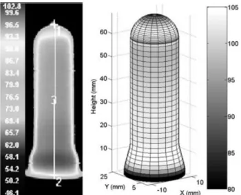
Figure 3 illustrates the external temperature distribution computed with the IR heating software, as well as the measured temperature cartography. To achieve more accu-rate comparisons, the temperature profile along the pre-form length at the end of the cooling step is represented in Fig. 4. We can observe a good agreement between
sim-ulations and measurements, since the maximum relative error is less than 5%. Figure 5 illustrates the variation of temperature versus time on a single point, located at 47 mm from the neck of the preform. This point was chosen because it corresponds to the node located at the middle height of the meshing. This curve shows clearly the effect of the cooling stage. Indeed, it is noticeable that after 3 s of cooling (also called inversion time), temperature on inner side becomes higher than on the outer side. This phenomenon can be easily explained; while natural con-vection tends to cool the external side, the internal side is heated by heat conduction. This point is crucial for the SBM process. Indeed, there can be a significant difference between the inside and outside hoop stretch ratios. To provide a good uniformity of the stress distribution through the thickness of the bottle, it is necessary to deliberately develop a nonuniform temperature profile throughout the preform before stretch and blowing [10]. Finally, Fig. 6 shows clearly that the temperature distribu-tion through the thickness is not linear, but exponential. At the end of the thermal conditioning step, the
tempera-FIG. 1. Blowing prototype: infrared oven, PET preform and instrumented mold.
TABLE 1. Process parameters of the IR oven. P1 (%) P2 (%) P3 (%) P4 (%) P5 (%) P6 (%) theat (s) tcool (s) 100 100 18 5 50 100 50 10
ture difference is approximately 48C. This value is never-theless strongly related to the cooling conditions.
The model is therefore able to predict suitably the tem-perature distribution of the preform at the end of the reheating stage. It allows examining the effect of process parameters on temperature profiles, especially through the preform wall thickness.
BLOW-MOLDING SIMULATION
Finite element analyses (FEA) of the SBM process were carried out using the commercial FE package ABA-QUS. In this section, we assess the ability of the above model to simulate the deformation process of a simple 18.5 g–50 cl PET bottle. A special attention was given to the measurement of both initial and boundary conditions, namely temperature, air pressure, and heat transfer coeffi-cient between the preform and the mold.
Boundary Conditions
The initial temperature distribution of the preform was calculated using the finite volume software previously presented. The heat transfer at the interface between the mold and the inflated preform is taken into account via a heat transfer coefficient h. A sensor to measure the heat transfer coefficient was developed for this study. The sen-sor as well as the method used for the measurements has been described in a previous article [29]. The peak value of h was related to the nominal air pressure imposed by the blowing device. As illustrated in Fig. 7, the heat trans-fer coefficient increases exponentially with the air pres-sure, and reaches an asymptotic value of 285 W m22K21 at a pressure of 10 bars. This coefficient is of prime inter-est since it drastically affects the cooling time of the bottle.
The air pressure inside the preform was measured as a function of time using a Kulite sensor (see Fig. 2). A
typ-FIG. 5. Variation of surface temperature versus time.
FIG. 6. Temperature profiles through the preform wall thickness. Same location as Fig. 4.
FIG. 3. External temperature distribution after cooling—(A) measured, (B) computed.
FIG. 4. External temperature profile along the preform length after 10 s cooling.
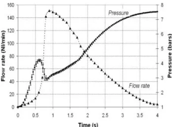
ical air pressure profile is illustrated in Fig. 8. We can observe a sharp increase in air pressure prior to deforma-tion. Once the preform begins to inflate, its enclosed vol-ume grows rapidly and, thus, the pressure drops. The pressure then increases steadily because of strain harden-ing and die-preform surface contact. After the preform is completely blown, the pressure reaches progressively a nominal value. This typical evolution of air pressure gives a good representation of the blowing kinematics. Menary et al. [24] have shown that applying the pressure directly as a boundary condition might lead to unrealistic results. Indeed, a pressure drop would induce a deflation of the preform, which is inconsistent with the rapid inflation observed experimentally. Actually, the pressure exerted by the air flow interacts with the preform, causing a de-formation of the structure, which in turn, alters the air flow itself by modifying the pressure. It is, therefore apparent from the above discussion, that it is crucial to model the fluid-structure interaction between the preform and the air flow, instead of considering the pressure as an input variable. In this work, we propose to account for the fluid-structure interaction using ‘‘hydrostatic fluid ele-ments’’ available in ABAQUS. At each time increment of the FE simulation, a thermodynamic model computes automatically the air pressure inside the preform. For that, the enclosed volume of the preform is modeled by a fluid-filled cavity whose temperature and pressure are sup-posed to be uniform. In addition, the fluid is assumed to behave like an ideal gas. Then, the volume of the cavity is calculated at each time increment using the coordinates of the bounded nodes. By assuming the cavity as a closed system subject to isothermal transformations, and by neglecting the fluid inertia, the volume–pressure compli-ance is given by the ideal gas law under hydrostatic con-ditions. The amount of air included in the cavity is assumed to be constant during each small time interval, but is updated at the end of the time increment using the value of the mass flow rate (MFR).
To estimate the MFR, Schmidt et al. [16] developed a thermodynamic model that formulates an explicit relation-ship between the MFR and the air pressure. In the case of an isovolume transformation (such transformation can be performed for instance by applying air pressure inside a rigid container), the MFR can be related to the initial slope of the pressure-versus-time curve. This method was, however, restricted to free blowing. In contrast, in the case of blow-molding, the MFR may be strongly time-de-pendent. Indeed, as illustrated by Fig. 8, the pressure inside the preform reaches an asymptotic value, which indicates clearly that the MFR decreases gradually to become null at the end of the blowing sequence. In this work, we measured the MFR as a function of time using a Bronkhorst hot wire sensor EL-FLOW1. Results of experiments are illustrated in Fig. 8.
Material Behavior
PET rheological behavior was modeled using the fol-lowing viscoplastic G’sell-WLF material model [30]:
s ¼ k0at
$
1& exp$& Ae%%exp&BeC'e˙m
with at¼ exp c1 & T& Tref ' c2þ T & Tref 8 > > > > > > : 9 > > > > > > ; (8)
where the equivalent Cauchy stressr depends on both the equivalent strain rate e, the cumulated strain e, and the_ temperature T. The sensitivity to the strain rate is taken into account via the parameter m, while (B, C) are hard-ening modulus. Finally,k0represents the consistence. This
model considers both temperature and strain rate depend-encies, as well as the strain hardening, which appears for large deformations. It presents the advantage to be numerically stable and relatively easy to implement. How-ever, this phenomenological behavior law is reserved to a
FIG. 7. Peak value of heat transfer coefficient versus nominal air pres-sure. The error bars show61 standard deviation for a set of nine trials.
FIG. 8. Variation of air pressure and mass flow rate versus time during the inflation step.
small range of temperature and strain rate. Besides, it takes into account neither the viscoelasticity of the mate-rial, nor the material orientation. We identified the consti-tutive parameters using an inverse method (nonlinear con-strain algorithm called sequential quadratic programming) from equi-biaxial tensile tests performed by Chavalier and Marco. [31]. The thermo-dependency was previously identified from shear tests on PET T74F9 [32]. We have implemented this model into ABAQUS via a Fortran sub-routine known as user creep.
Blow Molding FEM Model
Taking advantage of the bottle shape, we have adopted an axisymmetric model to reduce the computation times. In our application context, this approach is viable since both preform and mold designs are axisymmetric, as well as the loading applied on the structure. Previous studies investigated the effect of the preform meshing on the thickness distributions computed using FE simulations [33]. These studies have shown that shell elements can save a significant amount of CPU time in comparison with solid elements, while providing accurate results. In this work, however, we have adopted solid elements in order to provide an accurate calculation of the preform enclosed volume. Indeed, the coordinates of nodes used to mesh the inner surface of the preform are used to com-pute the enclosed volume. Thus, meshing the median
sur-face of the preform using shell elements would lead to a 30% overestimation of the preform enclosed volume, and consequently, a non-negligible error on the computed pressure, which is unacceptable. The preform is therefore meshed into 100 quadratic solid-elements (405 nodes), as illustrated in Fig. 9.
The mold used is a prototype developed at CROMeP. It produces 50 cl bottles. We assume this one to be rigid and isothermal. Indeed, for one SBM cycle, its tempera-ture increase is about 18C [29]. Figure 9 illustrates the mold geometry and the boundary conditions. To compute the heat transfer between the polymer and the mold, we have chosen a coupled temperature-displacement model in ABAQUS/Standard (implicit time integration scheme). Despite its potential effect on the blowing kinematics, the viscous dissipation is not calculated. In agreement with the blowing prototype, no stretch rod is modeled. Finally, the friction contact between the preform and the mold is assumed to be stick.
Results and Experimental Validation
One of the primary objectives of this section is to assess the consistency of the model with respect to the blowing kinematics. A way to proceed is to compare the pressure measured inside the bottle with the pressure computed by the model. The two pressure-versus-time profiles are illustrated in Fig. 10. There is a fair agree-ment in the trend between the two curves. The relative error between the measured pressure and the predicted one is approximately 16% at the end of the process. It is noticeable that the model successfully captures the drop in pressure measured at t ¼ 0.6 s. Besides, the drop in pressure corresponds to a rapid inflation of the preform. This can be seen in Fig. 11, which illustrates the interme-diate preform shapes versus time. This result is consistent with the observations reported in previous studies about the preform shape versus time, and its relationship with the measured pressure [16, 23, 24, 30]. We observe, how-ever, that the increase in slope in pressure-versus-time
FIG. 9. FE model—preform and mold geometries and boundary conditions.
curve, measured at approximately t ¼ 1.7 s, is predicted by the model at t ¼ 1.2 s. This might be a sign that the model underestimates the blowing time required to form the bottle.
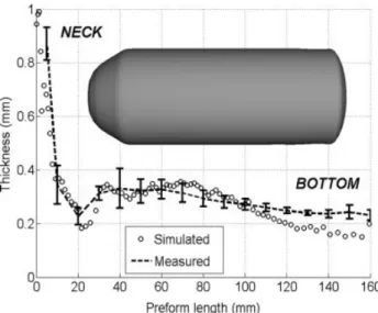
Figure 12 compares the thickness distribution calcu-lated numerically and the thickness profile measured experimentally. Measurements were averaged on a set of three trials. We observe a good agreement along most part of the bottle (less than 15% error on the mean thick-ness). The thickness predicted by the model remains nevertheless not thick enough at the bottle bottom. There are many possible causes for this: (i) excess stretch and distortion of elements around the corner makes the calcu-lation less accurate; (ii) the die-preform surface contact is assumed to be stick: this proscribes any sliding along the sidewall of the mold, which tends to decrease the thick-ness at the bottle bottom; and (iii) the injection point, located on the top of the preform, might be partially ther-mally crystallized. This might make the deformation of the corner difficult. Nevertheless, the model is capable of
predicting suitably the deformation process, and provides accurate predictions of the thickness distribution of the bottle, while respecting the blowing kinematics observed experimentally.
OPTIMIZATION OF PREFORM TEMPERATURE The performance of a bottle manufactured by SBM is drastically affected by its thickness distribution. To achieve bottles with appropriate thickness distributions, it is more desirable to adjust the process conditions, and to use the same design of preform for making different shapes of bottles. This approach aims to minimize the cost associated with the design of a new preform (espe-cially the manufacture of a new injection mold). Deter-mining adequate operating conditions remains neverthe-less costly and time consuming. Different approaches are possible, such as trial-and-error methods, or design of experiments. Both of them require a large number of experiments (or simulations), especially when the parame-ters are strongly interdependent. As a consequence, they become inadequate and impracticable for complex prob-lems. In contrast, the optimization algorithms make the optimization process fully automatic, and from this point of view, yield a significant assist in the development cycle.
In this section, we propose to couple an optimization algorithm to FE simulations in order to optimize the tem-perature distribution along the preform length. The goal will be to provide a homogeneous thickness for the bottle.
Parameterization and Constraints
To describe the temperature distribution along the pre-form length, we consider three optimization variables. They correspond to three temperatures located at different heights of the preform, as illustrated in Fig. 13. The whole
FIG. 11. Simulation of the intermediate bottle shapes.
FIG. 12. Wall thickness distribution of the bottle. The error bars show 1 standard deviation for a set of three trials.
FIG. 13. Temperature distribution along the preform length—optimiza-tion variables.
temperature distribution is then deduced using the Piece-wise Cubic Hermite Interpolating Polynomial (PCHIP) method [34]. To provide an accurate interpolation, an additional temperature is added on the preform neck. This fourth temperature is not optimized, but fixed to 808C, which corresponds approximately to the glass transition of PET. Indeed, throughout the reheating stage, the preform neck is generally protected from IR radiation in order to prevent its temperature from exceeding the PET glass transition. This approach aims to prevent any deformation of the bottle neck during the forming process. Finally, to simplify the problem, the temperature is assumed to be uniform through the preform thickness.
The optimization variables are constrained using lower and upper bounds, corresponding respectively to the PET glass transition temperature and to the PET crystallization temperature. These two physical limits have been natu-rally chosen to prevent serious rigidification of the struc-ture from appearing, in which case, any deformation would be proscribed during the forming stage. Let us note that neither linear nor nonlinear constraint is required.
Objective Function
In this application, we attempt to provide a uniform thickness for the bottle. This objective must be mathe-matically formulated by an appropriate cost-function. A simple way to proceed is to define the objective function F as the standard deviation of the computed thicknesses, as following: F$X%¼ 1 n& 1 Xn i¼1 ðthi& thÞ2 !1=2 (9)
where X represents the set of optimization variables, n is the number of nodes along the bottle height, thi is the
thickness at the nodei, and th is the mean thickness. The nodal thicknesses are computed using a Python script we developed into ABAQUS. Such a function is null for a bottle with perfectly uniform thickness.
Choice of an Algorithm
The choice of the optimization algorithm is closely related to the type of cost function. In our application, we attempt to minimize a nonlinear real-valued function, sub-ject to bound constraints. In addition, strong mechanical and geometric nonlinearities could induce significant nu-merical instabilities, making the objective-function noisy and therefore nondifferentiable. As a consequence, the gradient-based algorithms might not be adapted to this type of problem. In contrast, the direct-search methods (which do not require the computation of the cost-func-tion gradient) remain particularly adapted to the nonderi-vative optimization. Among this family of methods, the Nelder-Mead simplex algorithm is probably one of the
most popular. However, this local method provides rela-tively slow convergence rates [35]. Nevertheless, when the derivatives cannot be explicitly written, this method can save a significant amount of computation time com-pared with gradient-based methods. Indeed, the computa-tion of the cost-funccomputa-tion gradients can become strongly time consuming when they are approximated using the fi-nite-difference method. This is particularly true when the number of optimization variable is large.
In contrast, the Nelder-Mead simplex algorithm is re-stricted to unconstrained problems. In this work, we used the method proposed by Luersen and Riche [36] in order to add bound-constraints into the Nelder-Mead simplex algorithm available in Matlab1 [37].
RESULTS AND DISCUSSION
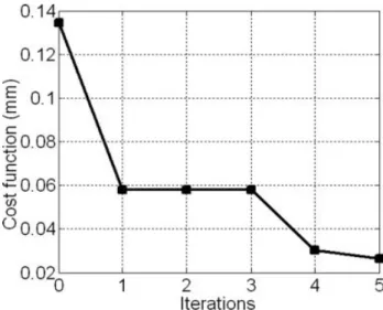
All numerical results reported in the sequel were obtained on a 2.8 GHz-512 Mo Pentium 4. Figure 14 dis-plays the decrease of the objective-function value in terms of the number of optimization iterations. We observe that the objective function is reduced by 60% of its initial value after the first iteration, and by more than 80% at the end of the optimization process. Consequently, the thickness distribution of the formed bottle is 80% more uniformed after optimization. The algorithm converges af-ter five iaf-terations, which involves only 10 objective-func-tion evaluaobjective-func-tions (that is to say, 10 FE simulaobjective-func-tions). On average, one cost-function evaluation requires 26 min CPU. Thus, the total CPU time required for the optimiza-tion is !3 h 20 min. Figure 15 illustrates the temperature distribution along the preform length before and after optimization. The corresponding values of the optimiza-tion variables are reported in Table 2. Initial condioptimiza-tions were chosen in order to apply a uniform temperature on the preform. Such temperature distribution leads to a strongly nonuniform thickness distribution for the bottle, as illustrated by Fig. 16. After optimization, there is a
temperature gradient along the preform length, which pro-vides a more uniform thickness, as illustrated by Fig. 16. In addition, Fig. 17 shows clearly that a uniform tempera-ture does not allow to fully blow the bottle (with the kinematics conditions previously presented). This problem is avoided with the optimized temperature profile, which provides a full blowing of the bottle. Figure 15 also illus-trates the optimal temperature distribution determined by Logoplast Company using an experimental trial-and-error method. This result has been obtained using the same pre-form, but with a different shape of mold. However, we can notice that there is a good agreement in the trends between the temperature profile experimentally deter-mined within industrial conditions, and the temperature distribution computed using our optimization method.
CONCLUSION
We have proposed in this work a modeling of the full SBM process. The IR heating step was simulated using a finite-volume software, whereas the deformation process was simulated using ABAQUS. All the boundary condi-tions required for the simulacondi-tions were carefully measured or calculated numerically. A major contribution of this work remains the modeling of the fluid-structure interac-tion existing between the preform and the air flow applied inside the preform. A numerical validation has shown that the model successfully captures the pressure-versus-time profile measured experimentally and provides an accurate prediction of the blowing kinematics. Future work will aim to further improve the model by using a more
power-ful constitutive law, which would account for the relation-ship between the temperature and the material orientation and crystallization.
As for SBM optimization, we proposed a practical methodology to numerically optimize the temperature dis-tribution of a PET preform, in order to provide a uniform thickness for the bottle. Encouraging preliminary results have shown the viability of our approach. However, it would probably be more desirable to directly optimize the process parameters of the heating systems. But to do so, both the IR heating simulation and the blowing simulation would need to be included into the optimization loop, resulting in further complications essentially due to long computation times. Nevertheless, this approach would im-plicitly account for the influence of the temperature
distri-TABLE 2. Optimization variables and cost function. T1 (8C) T2 (8C) T3 (8C) F (mm)
Initial 100 100 100 0.134
Final 110.7 98.9 92.9 0.026
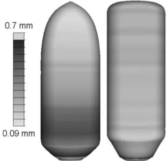
FIG. 16. Thickness distribution of the bottle before and after optimiza-tion.
FIG. 17. Bottle shapes and thickness distributions before and after opti-mization.
FIG. 15. Initial and optimized temperature distributions along the pre-form length.
bution through the preform thickness, which is of prime interest.
ACKNOWLEDGMENTS
This study was conducted within the frame of 6th EEC framework. STREP project APT_pack; NMP-PRIORITY 3. www.apt-pack.com. Special thanks to Logoplaste Tech-nology for manufacturing the preforms, and QUB for their collaboration. Authors also thank N. Billon, L. Chevalier, Y. Marco, G. Menary, V. Lucin, and C. Vallot for their contribution to this work.
REFERENCES
1. G. Venkateswaran, M.R. Cameron, and C.A. Jabarin, Adv. Polym. Technol., 17, 237 (1998).
2. S. Monteix, Y. Le Maoult, and F. Schmidt,QIRT J., 1, 133 (2004).
3. H.-X. Huang, Y.-Z. Li, and Y.-H. Deng,Polym. Test., 25, 6 (2006).
4. H.-X. Huang, Y.-H. Deng, and Y.-F. Huang, SPE ANTEC Technical Papers, Boston, USA, 12 (2005).
5. C. Champin, M. Bellet, F.M. Schmidt, J.-F. Agassant, and Y. Le Maoult, 3D Finite Element Modeling of the Blow Molding Process, 8th ESAFORM Conference on Material Forming, Cluj-Napoca, Romania, Vol. 2, 905 (2005). 6. W. Michaeli and W. Papst, ‘‘FE-Analysis of the Two-Step
Stretch Blow Molding Process,’’ inSPE ANTEC Technical Papers 30, Chicago, USA (2004).
7. S. Monteix, F. Schmidt, Y. Le Maoult, R.B. Yedder, R.W. Diraddo, and D. Laroche, J. Mater. Proc. Tech., 119, 1 (2001).
8. R. DiRaddo and A. Garcia-Rejon,Plast. Rubb. Comp. Proc. Appl., 20 (1993).
9. L. Martin, D. Stracovsky, D. Laroche, A. Bardetti, R. Ben-Yedder, and R. DiRaddo, ‘‘Modeling and Experimental Val-idation of the Stretch Blow Molding of PET,’’ in SPE ANTEC Technical Papers, New York (1999).
10. P.H. Lebaudy and J. Grenet,J. Appl. Polym. Sci., 80, 2683 (2001).
11. S. Wang, A. Makinouchi, and T. Nakagawa, Adv. Polym. Tech., 17, 3 (1998).
12. F. Thibault, A. Malo, B. Lanctot, and R. Diraddo, Polym. Eng. Sci., 47, 3 (2007).
13. F.M. Schmidt, J.-F. Agassant, M. Bellet, and L. Desoutter, J. Non-Newtonian Fluid Mech., 64, 19 (1996).
14. K. Chung,J. Mater. Shaping Technol., 9 (1998).
15. J.P. McEvoy, C.G. Armstrong, and R.J. Crawford, Adv. Polym. Technol., 17, 339 (1998).
16. F.M. Schmidt, J.F. Agassant, and M. Bellet, Polym. Eng. Sci., 38, 9 (1998).
17. S. Wang,Int. Polym. Proc., 15, 166 (2000).
18. Z.J. Yang, E. Harkin-Jones, G.H. Menary, and C.G. Arm-strong,Polym. Eng. Sci., 44, 7 (2004).
19. X.-T. Pham, F. Thibault, and L.-T. Lim, Polym. Eng. Sci., 44, 8 (2004).
20. S. Wang, A. Makinouchi, and T. Nakagawa,Int. J. Numer. Methods Eng., 48, 501 (2000).
21. F. Erchiqui,Polym. Eng. Sci., 46, 11 (2006).
22. E. Verron, G. Marckmann, and B. Peseux, Int. J. Numer. Methods Eng., 50, 1233 (2001).
23. H. Mir, Z. Benrabah, and F. Thibault, ‘‘9th International Conference on Numerical Methods in Industrial Forming Processes,’’ inAIP Conference Proceedings, Porto, Portugal, Vol. 908, 331 (2007).
24. G. Menary, C.W. Tan, M. Picard, N. Billon, C.G. Arm-strong, and E.M.A. Harkin-Jones, ‘‘10th ESAFORM Confer-ence on Material Forming,’’ inAIP Conference Proceedings, Zaragoza, Spain, Vol. 907, 939 (2007).
25. D.K. Lee and S.K. Soh,Polym. Eng. Sci., 36, 11 (1996). 26. M. Bordival, F.M. Schmidt, and Y. Le Maoult, ‘‘Numerical
Modeling and Optimization of Infrared Heating System for the Blow Molding Process,’’ in 9th ESAFORM Conference on Material Forming, Glasgow, UK, 511 (2006).
27. M. Modest, Radiative Heat Transfer, McGraw-Hill, New York (1993).
28. F.P. Incropera, Fundamentals of Heat and Mass Transfer, Wiley, New York, 546 (1985).
29. M. Bordival, F.M. Schmidt, and Y. Le Maoult, ‘‘10th ESA-FORM Conference on Material Forming,’’ in AIP Confer-ence Proceedings, Zaragoza, Spain, Vol. 907, 1245 (2007). 30. C.G’ Sell and J. Jonas,J. Mater. Sci., 14, 583 (1979). 31. L. Chevalier and Y. Marco,Mech. Mater., 39, 596 (2007). 32. E. Gorlier, ‘‘Caracte´risation Rhe´ologique Et Structurale d’un
PET. Application Au Proce´de´ de bi-e´tirage Soufflage de Bouteilles,’’ Ph.D. Thesis, in French, ENSMP (2001). 33. G. Menary, ‘‘Modeling of Injection Stretch Blow Molding
and the Resulting In-Service Performance of PET Bottles,’’ Ph.D. Thesis, QUB (2001).
34. F.N. Fritsch and R.E. Carlson,SIAM J. Numer. Analysis, 17, 238 (1980).
35. J.C. Lagarias, J.A. Reeds, M.H. Wright, and P.E. Wright, SIAM J. Optimization, 9, 1 (1998).
36. M.A. Luersen and R. Le Riche, ‘‘Globalized Nelder-Mead Method for Engineering Optimization,’’ in Proceedings of the Third International Conference on Engineering Compu-tational Technology, Stirling, Scotland, 165 (2002).
37. The MathWorks, User’s Guide, Optimization Toolbox For Use With Matlab, Version 2 (2002).