A new 3D-matching method of non-rigid and partially similar models using curve analysis

HAL Id: hal-00660801

https://hal.archives-ouvertes.fr/hal-00660801

Submitted on 17 Jan 2012

HAL is a multi-disciplinary open access

archive for the deposit and dissemination of

sci-entific research documents, whether they are

pub-lished or not. The documents may come from

teaching and research institutions in France or

abroad, or from public or private research centers.

L’archive ouverte pluridisciplinaire HAL, est

destinée au dépôt et à la diffusion de documents

scientifiques de niveau recherche, publiés ou non,

émanant des établissements d’enseignement et de

recherche français ou étrangers, des laboratoires

publics ou privés.

A new 3D-matching method of non-rigid and partially

similar models using curve analysis

Hedi Tabia, Mohamed Daoudi, Jean-Philippe Vandeborre, Olivier Colot

To cite this version:

Hedi Tabia, Mohamed Daoudi, Jean-Philippe Vandeborre, Olivier Colot. A new 3D-matching method

of non-rigid and partially similar models using curve analysis. IEEE Transactions on Pattern Analysis

and Machine Intelligence, Institute of Electrical and Electronics Engineers, 2011, 33 (4), pp.852-858.

�10.1109/TPAMI.2010.202�. �hal-00660801�

A new 3D-matching method of non-rigid and

partially similar models using curve analysis

Hedi Tabia, Mohamed Daoudi, Jean-Philippe Vandeborre and Olivier Colot

✦

Abstract—The 3D-shape matching problem plays a crucial role in

many applications such as indexing or modeling by example. Here, we present a novel approach to match 3D-objects in presence of non-rigid transformation and partially similar models. In this paper, we use the representation of surfaces by 3D-curves extracted around feature points. Indeed, surfaces are represented with a collection of closed curves and tools from shape analysis of curves are applied to analyze and to compare curves. The belief functions are used to define a global distance between 3D-objects. The experimental results obtained on the TOSCA and the SHREC07 datasets show that the system efficiently performs in retrieving similar 3D-models.

Index Terms—3D-shape matching, Curves analysis, Belief functions,

Feature points.

1

I

S

in analyzing shapes of three-dimensional (3D) ob-jects. Advances in 3D scanning technologies, hardware-accelerated 3D graphics, and related tools, are enabling access to high quality 3D data. As technologies are im-proving, the need for automated methods for analyzing shapes of 3D-objects is also growing. Shape matching remains a central technical problem for efficient 3D-object search engine design. It plays an important role in many applications such as computer vision, shape recognition, shape retrieval and computer graphics.

In recent years, a large number of papers are con-cerned in shape matching. Most of the current 3D-shape matching approaches are based on global similar-ity. Some methods directly analyze the 3D-mesh — such as Antini et al. [1] who use curvature correlograms — and some others use a 2D-view based approach — such as Filali et al. [2] who propose an adaptive nearest neighbor-like framework to choose the characteristic views of a 3D-model. These approaches enable retrieval of similar objects in spite of rigid transformations. Other approaches are also enabling retrieval of objects that differ from non-rigid transformations such as shape bending or character articulation [3]. They are generally based on the graph or skeleton computation of a 3D-object [4], [5].

H. Tabia and O. Colot are with LAGIS FRE CNRS 3303 / University Lille 1, France. M. Daoudi and J-P. Vandeborre are with TELECOM Lille 1; Institut TELECOM / LIFL UMR CNRS 8022 / University Lille 1, France.

Other case of shape matching is encountered when partially similar shapes are presented. This kind of shape matching plays a crucial role in many applications such as indexing or modeling by example. It is usually ap-proached using the recognition by part idea [6], [7]: seg-mentation of the shape in significant parts, and matching pairs of parts as whole shapes. Bronstein et al. [8] also proposed to consider the 3D-matching problem as a multi-criterion optimization problem trying to simulta-neously maximize the similarity and the significance of the matching parts.

In this paper, we present a new approach for 3D-object matching based on curve analysis. An important line of work in face analysis has been to use shapes of curves that lie on facial surfaces [9], [10]. However, these works have been intended for face recognition only and not for shape analysis of generic 3D-surfaces. Our approach consists to represent 3D-objects as a set of parts. Each part is represented by an indexed collection of closed curves in R3on the 3D-surface. Then we use shape anal-ysis of curves in the matching process. First of all, given a 3D-object, a set of feature points is extract. Around each feature point, a set of closed curves is automatically computed. One feature point and its associated set of curves is called a 3D-part. Curves are level curves of a surface distance function defined to be the length of the shortest path between that point and the feature point. This function is stable with respect to changes in non-rigid transformations. In this paper, we analyze the shape of 3D-part surfaces by analyzing the shape of their corresponding curves. The belief functions are used to define a global distance between 3D-objects using the distance between their corresponding 3D-parts.

The paper is organized as follows. A feature point extraction algorithm, using geodesics, is introduced in the next section. Section 3 describes our framework for feature descriptors building, and explains how a set of curves is associated to each feature point already extracted. This section also presents a step-by-step proce-dure to compare 3D-part surfaces using the correspond-ing curves. In section 4, we exploit the previously pre-sented 3D-part surface comparison schema to propose a 3D-object matching method using fusion tools given by belief function theory. In section 5, experimental results

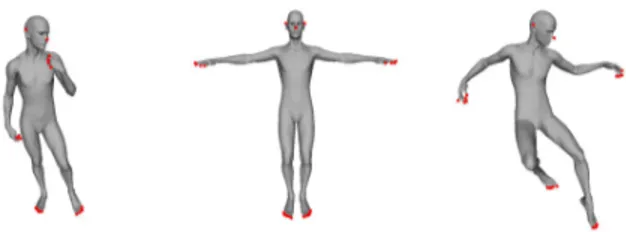
Fig. 1. Feature points extracted from different poses of 3D-model.

are shown. Finally, section 6 contains the concluding remarks.

2

F

In this section, we present the algorithm used in the feature point extraction process. This algorithm is based on topological tools proposed by Tierny et al. [6]. Us-ing a diversity of 3D-surfaces, the proposed algorithm produces robust and well-localized feature points. The concept of feature points has been introduced by several authors [11], [12]. However it is difficult to find a formal definition that characterizes this concept. In Katz et al. [12] feature points refer to the points localized at the extremity of a 3D-surface’s components. Formally, feature points are defined as the set of points that are the furthest away (in the geodesic sense) from all the other points of the surface. They are equivalent to the local extrema of a geodesic distance function which is defined on the 3D-surface. Figure 1 shows some 3D-surfaces with their corresponding feature points.

Let v1 and v2 be the farthest vertices (in the geodesic

sense) on a connected triangulated surface S. Let f1 and

f2 be two scalar functions defined on each vertex v of

the surface S , as follows: f1(v) = δ(v, v1) and f2(v) =

δ(v, v2) where δ(x, y) is the geodesic distance between

points x and y on the surface.

As mentioned by [13], in a critical point classification, a local minimum of fi(v) is defined as a vertex vmin such

that all its level-one neighbors have a higher function value. Reciprocally, a local maximum is a vertex vmax

such that all its level-one neighbors have a lower func-tion value. Let F1be the set of local extrema (minima and

maxima) of f1 and F2 be the set of local extrema of f2.

We define the set of feature points F of the triangulated surface S as the closest intersecting points in the sets F1

and F2. In practice, f1and f2local extrema do not appear

exactly on the same vertices but in the same geodesic neighborhood. Consequently, we define the intersection operator ∩ with the following set of constraints, where δn stands for the normalized geodesic distance function

(to impose scale invariance):

V ∈ F = F1∩ F2⇔        ∃vF1 ∈ F1 / δn(V, vF1) < ǫ ∃vF2 ∈ F2 / δn(V, vF2) < ǫ δn(V, vi) > ǫ ∀vi ∈ F ǫ, δn∈ [0, 1]

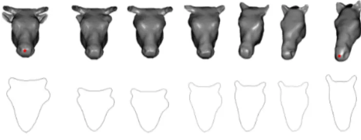
Fig. 2. 3D-curves on horse model extracted around its feature points.

This algorithm detects all the feature points required in the subsequent analysis. They are accurately localized and their localization is robust with respect to rigid and non-rigid transformations, because of the use of geodesic distance in f1 and f2 functions. In the experimental

section, we will evaluate the localization accuracy of feature points detection within our global approach.

3

F

As mentioned earlier, our goal is to analyze shapes of 3D-surfaces using shapes of curves extracted around a set of feature points. In other words, we divide a 3D-surface into a set of parts. Each parts consists of one feature point and an indexed collection of simple, closed curves in R3_{. The geometry of 3D-parts is then studied}

using the geometries of the associated curves. Curves are defined as level curves of an intrinsic distance function on the 3D-part surface. Their geometries in turn are invariant to the rigid transformations of the 3D-part surface. These curves jointly contain all the information about the surface and it is possible to go back-and-forth between the surface and the curves without any ambiguity. In this section, we firstly describe how to extract a significant set of curves around feature points. We explain then the framework of curves analysis and its extension to comparison of 3D-part surfaces. Let Vibe

a feature point on a 3D-triangulated surface. A geodesic distance function is defined on that 3D-surface such that Vibe its origin. The geodesic function is split into a set of

levels. Vertices which are in the same level are extracted with respect to an arbitrary order. Let λ be a level set corresponding to the geodesic distance function f . The set of ordered vertices v such that f (v) = λ builds one curve. Figure 2 shows the sets of curves corresponding to the horse’s feature points.

3.1 Curves analysis

The analysis of 3D-shapes via their associated curve space has a technical sound foundation in the Morse theory [14]. In our approach, we treat curves as closed, parameterized in R3 _{and we rescale them to have the}

same length, say 2π. This allows us to use one of many methods already available for elastic analysis of closed curves.

Several authors, starting with Younes [15], followed by Michor and Mumford [16] and others, have studied curves for planar shapes. More recently Joshi et al. [17] have extended it to curves in Rn _{using an efficient}

and Mennucci [18], have also used Riemannian metrics on curve spaces. Their main purpose was to study curves evolution rather than shape analysis. Here, we adopt the Joshi et al’s approach [17] because it simplifies the elastic shape analysis. The main steps are: (i) define a space of closed curves of interest, (ii) impose a Riemannian structure on this space using the elastic metric, and (iii) compute geodesic paths under this metric. These geodesic paths can then be interpreted as optimal elastic deformations of curves.

We start by considering a closed curve β in R3_.

Since it is a closed curve, it is parameterizable using β : S1 _{→ R}3_{. We will assume that the parameterization}

is non-singular, i.e. k ˙β(t)k 6= 0 for all t. The norm used here is the Euclidean norm in R3_{. Note that the}

parameterization is not assumed to be arc-length; we allow a larger class of parameterizations for improved analysis. To analyze the shape of β, we shall represent it mathematically using a square-root velocity function (SRVF), denoted by q(t), according to: q(t)=. √β(t)˙

k ˙β(t)k.

q(t) is a special function that captures the shape of β and is particularly convenient for shape analysis, as we describe next. Firstly, the squared L2-norm of q, given by: kqk2 ₌ R

S1hq(t), q(t)i dt =

R

S1k ˙β(t)kdt , which is

the length of β. Therefore, the L2-norm is convenient to analyze curves of specific lengths. Secondly, as shown in [17], the classical elastic metric for comparing shapes of curves becomes the L2_{-metric under the SRVF}

repre-sentation. This point is very important as it simplifies the calculus of elastic metric to the well-known calculus of functional analysis under the L2_{-metric. In order to}

restrict our shape analysis to closed curves, we define the set: C = {q : S1 _{→ R}3_|R

S1q(t)kq(t)kdt = 0} ⊂

L2_(S1_{, R}3_{) .}

Here L2_(S1_{, R}3_{) denotes the set of all functions from}

S1 _{to R}3 _{that are square integrable. The quantity}

R

S1q(t)kq(t)kdt denotes the total displacement in R

3 _as

one traverses along the curve from start to end. Setting it equal to zero is equivalent to having a closed curve. Therefore, C is the set of all closed curves in R3_{, each}

represented by its SRVF. Notice that the elements of C are allowed to have different lengths. Due to a nonlinear (closure) constraint on its elements, C is a nonlinear manifold. We can make it a Riemannian manifold by using the metric: for any u, v ∈ Tq(C), we define:

hu, vi = Z

S1hu(t), v(t)i dt .

(1) We have used the same notation for the Riemannian metric on C and the Euclidean metric in R3 _{hoping that}

the difference is made clear by the context. For instance, the metric on the left side is inC while the metric inside the integral on the right side is in R3_{. For any q ∈ C,}

the tangent space: Tq(C) = {v : S1 → R3| hv, wi =

0, w ∈ Nq(C)} , where Nq(C), the space of normals at q is

given by: Nq(C) = span{q

1 (t) kq(t)kq(t) + kq(t)ke1, q2 (t) kq(t)kq(t) +

form an orthonormal basis of R3.

It is easy to see that several elements ofC can represent curves with the same shape. For example, if we rotate a curve in R3_{, we get a different SRVF but its shape}

remains unchanged. Another similar situation arises when a curve is re-parameterized; a re-parameterization changes the SRVF of curve but not its shape. In order to handle this variability, we define orbits of the rotation group SO(3) and the re-parameterization group Γ as the equivalence classes in C. Here, Γ is the set of all orientation-preserving diffeomorphisms of S1 (to itself) and the elements of Γ are viewed as re-parameterization functions. For example, for a curve β : S1 _{→ R}3 _and

a function γ : S1 _{→ S}1_{, γ ∈ Γ, the curve β(γ) is a}

re-parameterization of β. The corresponding SRVF changes according to q(t) 7→ p ˙γ(t)q(γ(t)). We set the elements of the set: [q] = {p ˙γ(t)Oq(γ(t))|O ∈ SO(3), γ ∈ Γ} , to be equivalent from the perspective of shape anal-ysis. The set of such equivalence classes, denoted by S = C/(SO(3) × Γ) is called the shape space of closed. curves in R3. S inherits a Riemannian metric from the larger spaceC and is thus a Riemannian manifold itself. The main ingredient in comparing and analyzing shapes of curves is the construction of a geodesic between any two elements of S, under the Riemannian metric given in Eqn. 1. Given any two curves β1 and β2, represented

by their SVRFs q1and q2, we want to compute a geodesic

path between the orbits [q1] and [q2] in the shape space

S. This task is accomplished using a path straightening approach which was introduced in [19]. The basic idea here is to connect the two points [q1] and [q2] by an

arbitrary initial path α and to iteratively update this path using the negative gradient of an energy function E[α] = 1₂R

sh ˙α(s), ˙α(s)i ds. The interesting part is that

the gradient of E has been derived analytically and can be used directly for updating α. As shown in [19], the critical points of E are actually geodesic paths in S. Thus, this gradient-based update leads to a feature point of E which, in turn, is a geodesic path between the given points. We will use the notation d(β1, β2) to denote

the geodesic distance, or the length of the geodesic in S, between the two curves β1 and β2. Shown in the

bottom row of Figure 3 is an example of geodesic path between two curves extracted from two different 3D-part surfaces; the cow-head 3D-part (left side) and the horse-head part (right side).

3.2 3D-Parts matching

Now we extend ideas developed in the previous section for analyzing shapes of curves to the shapes of full 3D-part surfaces. As mentioned earlier, a 3D-3D-part surface P is represented with an indexed collection of the level curves of the f function. That is, P is equivalent to the set {cλ∈ [0, L]}, where cλis the level set associated with the

distance function value equal to λ. Through this relation, each 3D-part has been represented as an element of the

Fig. 3. Geodesic path between cow-head part and horse-head part.

setC[0,L]_{. In our framework, the shapes of any two parts}

are compared by comparing their corresponding curves. Lets D denotes the global distance between two parts.

Given any two surfaces parts P1 and P2, and their

collection of curves {c1λ, λ ∈ [0, L]} and {c2λ, λ ∈ [0, L]},

respectively, our idea is to compare the curves c1λand c2λ,

and to accumulate these distances over all λ. Formally, we define a distance: D :C[0,L]_{× C}[0,L]_{→ R} ≥0, given by D(P1, P2) = Z L 0 d(c1λ, c2λ)dλ.

Here, the distance inside the integral is the geodesic distance function between the shapes of any curves, described in the last section. In Figure 3, The top row shows the two 3D-part surfaces (cow-head and horse-head) and the resulting geodesic path between them. Middle surfaces denote five equally spaced points (in the space of all parameterized paths) along the geodesic path. With respect to the chosen Riemannian metric, this path denotes the optimal deformation from the cow-head part to the horse-cow-head part.

4

3D-

In this section, we use the proposed 3D-parts matching method in order to compute a global distance between 3D-objects. For that, a fusion method based on the Trans-ferable Belief Model (TBM) framework [20], an interpreta-tion of the Dempster-Shafer theory of evidence, is pro-posed and applied to perform the 3D-shape matching. The TBM is shown to provide a powerful framework, well suited to the merge process.

4.1 Transferable Belief Model concept

The TBM is based on a two-level model: a credal level where beliefs are entertained, combined and updated, and a pignistic level where beliefs are converted into probabilities to make decisions.

4.1.1 Credal level

Let Ω denote a finite set called the frame of discernment. A Basic Belief Assignment (BBA) or mass function is a function m : 2Ω _{→ [0, 1], such that:} P

A⊆Ωm(A) = 1

m(A) measures the amount of belief that is committed

to A. The subsets A of Ω such that m(A) > 0 are called focal elements.

Given two BBAs m1 and m2 defined over the same

frame of discernment Ω and induced by two distinct pieces of information, we can combine them using the Dempster Shafer Combination rule [21] given by:

(m1⊗ m2)(A) = X B∩C=A m1(B)m2(C). (2) for all A⊆ Ω. 4.1.2 Pignistic level

When a decision has to be made, the beliefs held at the credal level induce a probability measure at the pignistic level. Hence, a transformation from belief functions to probability functions must be done. This transformation is called the pignistic transformation. Let m be a BBA defined on Ω, the probability function induced by m at the pignistic level, denoted by BetP and also defined on Ω is given by:

BetP (ω) = X

ω∈A

m(A)

|A| (3)

for all ω ∈ Ω and where |A| is the number of elements of Ω in A.

4.2 3D-shape matching

Given a collection of M 3D-objects Ω ={Oj, 1 ≤ j ≤ M}

and a set of N 3D-object parts{Pi, 1 ≤ i ≤ N} extracted

from a global 3D-object query Q, our aim is to compute a global similarity metric between the 3D-object query Q and 3D-objects in the collection. This metric is based on the distance between parts presented in Section 3. In order to achieve this computation, each part Pi is

modeled by one BBA mPi. This BBA is defined on Ω

as frame of discernment and it measures the amount of belief accorded to the assumption: Pi belongs to Oj.

Formally, mPi is a mass function 2

Ω_{→ [0, 1] given by:} mPi(Oj) = µ(Pi) · 1 − D1(Pi, Oj) PM l=1(1 − D1(Pi, Ol)) (4) mPi(Ω) = 1 − µ(Pi)

where D1 is a distance measure defined between an

object part Pi of the query Q and a global 3D-object Oj

in the collection. This measure represents the distance between the part Pi and its closest one in Oj. Formally

D1 is given by:

D1(Pi, Oj) = min k,Pk⊂Oj

(D(P, Pk)) (5)

It is required to normalize this distance in order to obtain a distribution on [0, 1] which allows us a correct construction of the BBA.

In equation 4, µ(Pi) is a confidence coefficient on [0,1].

This coefficient is interpreted as the significance given to each part in a global 3D object.

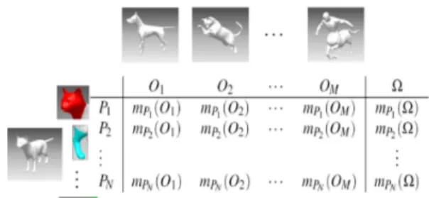
Fig. 4. Cat parts and their respective BBAs.

As mentioned by Bronstein et al. [8], the quantifica-tion of the significance of an object’s part is a major challenge. Here, we define the significance of a shape’s part as a function of the partiality function used in [8]. The value µ(Pi) of a 3D-part can be computed as

µ(Pi) = exp(−npartiality(Pi)2) where npartiality is the

normalized partiality function of the 3D-part Pi. It is

given by npartiality(Pi) =area(Q)−area(P_area(Q) i).

When all parts Pi of the query Q are modeled by

their corresponding mass functions, we can apply the Dempster Shafer combination rule in order to get a mass function which measures the amount of belief committed to the assumption: Q is similar to Oj.

Lastly, a decision is made from the obtained BBA and resulting objects are sorted based on a pignistic probability distribution. Our approach is summarized in algorithm 1 and depicted in Figure 4. In this figure a 3D-object of a cat is divided into several parts Pi. A mass

distribution BBA is constructed for each part over all objects in the collection. The combination of all masses gives us a similarity indication about the whole object with all objects in the collection.

Algorithm 1 : 3D-shape search algorithm

Given a 3D-object query Q.

1: Extract a set of N feature points Vifrom Q.

2: foreach feature point Viwhere i = 1, ..., N do

3: Extract a set of closed curves (ie. part Pi).

4: Compute the distance between Piand all objects in Ω using

eq 5.

5: Set a BBA value for all the objects mPi(Oj) using eq 4.

6: end for

7: Combine all BBAs mPi into a new BBA mQusing eq 2.

8: Compute the pignistic probability induced by mQusing eq 3.

9: Display 3D-objects in the order according to the pignistic prob-ability.

5

E

R

In this section, we present the databases, some state-of-the-art shape-matching algorithms to compare with, the evaluation criteria and the experimental results. Data with noise are considered in the sequel and a quanti-tative analysis of the experimental results are reported. The algorithms that we have described in the previous

sections have been implemented using MATLAB

soft-ware. The framework encloses an off-line feature point

and an on-line retrieval process. To evaluate our method, we used two different databases. The TOSCA data set for non-rigid shapes and the SHREC07 shape benchmark for partially similar models.

5.1 TOSCA data set description

The TOSCA1_{data set has been proposed by Bronstein et}

al. [22]. It is an interesting database for non-rigid shape correspondence measures. The database consists of 148 models, enclosing 12 classes. Each class contains one 3D-shape under a variety of poses (between 1 and 20 poses for each class). This classification is provided with the data set.

5.2 SHREC07 data set description

This benchmark2 _{is composed of a dataset of 400}

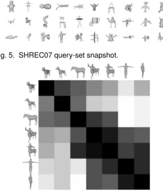
man-ifold models and of a query set of 30 manman-ifold models composed of composite models as shown in Figure 5. Hence, it is an interesting database for partial shape retrieval. The dataset exhibits diverse variations, from pose change, to shape variability within a same class or topology variation (notice 4 of the 20 classes contain non zero genus surfaces) [23]. The ground truth is provided with the data set.

5.3 Some state-of-the-art algorithms

In order to evaluate the 3D-global matching approach, we compare our method with some state-of-the-art shape-matching algorithms.

• Extended Reeb Graphs (ERG): it is a structural

based 3D matching method. It works with Reeb graph properties [23].

• Ray-based approach with Spherical Harmonic

rep-resentation (RSH): Saupe and Vranic [24] use PCA to align the models into the canonical position. Then the maximal extents are extracted, and finally the spherical harmonic is applied.

• The hybrid feature vector(DSR): it is a combination

of two view based descriptors: the depth buffer and the silhouette and radialized extent function descriptor [25].

• The Geodesic D2: it is an extension of the Euclidean

D2 [26]. It is computed as a global distribution of geodesic distances in 3D-shapes.

5.4 Evaluation criterion

There are several different performance measures which can evaluate retrieval methods. In this paper, we test the robustness of our approach using the Precision vs Recall plots. They are well known in the literature of content-based search and retrieval. The precision and recall are defined as follow: P recision =N A, Recall = N Q 1.http://tosca.cs.technion.ac.il/ 2.http://partial.ge.imati.cnr.it/

Fig. 5. SHREC07 query-set snapshot.

Fig. 6. Matrix of pairwise distances between seven 3D-objects.

where N is the number of relevant models retrieved in the top A retrievals, Q is the number of relevant models in the collection, which is the number of models to which the query belongs to.

5.5 Results

During the off-line process each model in the database has been remeshed to get a regular model. Feature points have been extracted and their related sets of curves (parts) have been extracted and stored into indexed files. During the on-line process, feature points and related curves of the query object are extracted.

5.5.1 Results on the TOSCA dataset

In order to show the main contribution of our approach, some results are shown as a matrix in Figure 6. In this visualization of the matrix, the lightness of each element (i; j) is proportional to the magnitude of the distances between 3D-objects i and j. That is, each square, in this matrix, represents the distances between two 3D-objects. Darker elements represent better matches, while lighter elements indicate worse matches.

This matrix is not symmetric because our similarity measure based on belief function is not symmetric either. In this matrix, humans are similar together and partially similar to centaurs. Centaurs are similar together and partially similar to horses and humans. According to the lightness of the matrix square, we can easily do the distinction between three different classes. The first class contains the first three animals, the second class encloses centaurs and horse and the third class contains humans and centaurs.

Fig. 7. First retrieved results on the TOSCA dataset.

Fig. 8. Precision vs Recall plots comparing our approach to RSH, D2 and DSR algorithms on the TOSCA dataset.

Other visual results are shown in Figure 7. The first column contains the query while the rest are the four retrieved 3D-objects. An interesting result is shown in the last row of Figure 7, where the query is a centaur, the forth retrieved 3D-object is a horse which is partially similar to the centaur.

Quantitative analysis of our experimental results are depicted in Figure 8. Figure 8 shows the Precision vs Recall plots for our approach and some well-known descriptors. We find that our approach provides the best retrieval precision in this experiment.

5.5.2 Results on the SHREC07 dataset

From a qualitative point of view, Figure 9 gives a good overview of the efficiency of the framework. For exam-ple, in the first row, the query is a centaur and thus most of the top-results are humanoid and animal models.

Quantitatively, we compare the Precision vs Recall plot of our approach with other methods competing the contest. Such a plot is the average of the 30 Precision vs Recall plots corresponding to the 30 models of the query-set. Figure 10 shows the these plots. As the curve of our approach is higher than the others, it is obvious that it outperforms related methods.

5.6 Robustness to query noises

We investigate the framework robustness against surface noise. For each element of the query-set, we added a surface noise. The noise is±0.2% and ±0.5% the length of the model’s bounding box. It consists of three random

Fig. 9. First retrieved results on the SHREC07 dataset.

Fig. 10. Precision vs Recall plot on the SHREC07

dataset.

translations in the three directions X, Y and Z. Figure 11 shows some examples of the noise effect.

Precision vs Recall plot are computed for our approach under the noise and compared with the original Preci-sion vs Recall plot. From this results shown in Figure 12, the noise addition effects can be observed. These plots demonstrate the stability of the algorithm despite random noise. Moreover, even with a random noise of ±0.5% it still outperforms the scores on clean data of two methods presented in Figure 8.

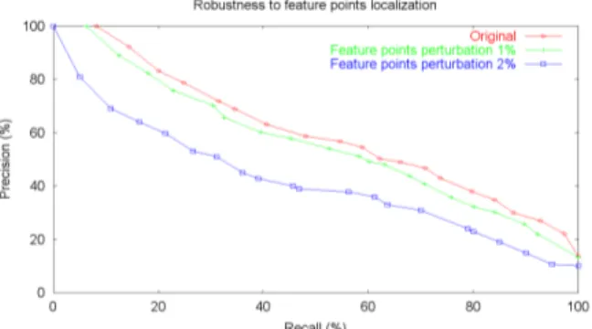
5.7 Robustness to feature points localization

In order to assess the robustness of our method under localization of feature points, we apply the following transformation for the query set. We select a random vertex located in a geodesic radius (1% and 2% of the geodesic diameter of the 3D-object) centered in the original feature points.

In Figure 13 an example of the feature points localiza-tion with noise addilocaliza-tion is shown. The original feature point is colored in green. The perturbation consists of a

Fig. 11. Surface noise on a TOSCA 3D-model: Original, ±0.2% noise and ±0.5% noise (from left to right).

Fig. 12. Robustness to query noises on the TOSCA

dataset.

Fig. 13. An example of the feature point location with perturbation (1% bottom and 2% top).

random selection of one vertex among vertices colored in red. Figure 14 shows that the performance of our approach is robust with respect to 1% of perturbation. The 2% perturbation plot shows the limit of the algo-rithm in term of feature point perturbation. However our method performance is still comparable to state-of-the-art method performance on clean data.

5.8 Discussion and limitations

The feature point extraction step of the framework, which is based on geodesics, introduces a bias in the comparison process. To guarantee stability and perfor-mance, this method has to be stable within a same class of objects and moreover coherent with the dataset ground-truth. In practice, with the TOSCA and the SHREC07 datasets, feature extraction turns out to be ho-mogeneous within most classes. However, the geodesic

Fig. 14. Robustness to feature points localization on the TOSCA dataset.

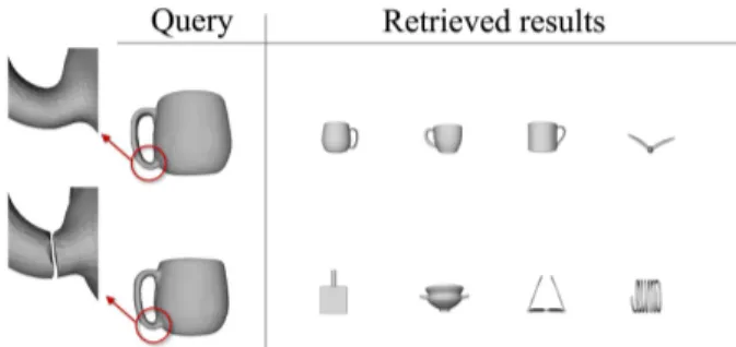
Fig. 15. First retrieved results of a 3D-query with topolog-ical noise addition (The original query is on the top). metric is known to be very sensitive to topology which make the overall framework quite sensitive to topology variations also. Figure 15 shows the same query under topological change. In the first row, when the query genus is 1, the system performs retrieval effectively. However, the second query which represents the same cup with added topological noise (genus is 0), shows dif-ferent results. In the future, we would like to investigate other decomposition strategies that would overcome this issue using more robust metrics such as the diffusion or the commute time distances [27] or using methods from the 2D shape analysis for finding interest points and choosing features [28]. Moreover, because of the use of curve descriptors, the 3D-objects in the database must be of quite high quality (manifold and high resolution).

6

C

In this paper, we have presented a geometric analysis of 3D-shapes in presence of non-rigid transformation and partially similar models. In this analysis, the preprocess-ing is completely automated: the algorithm processes the 3D-object, extracts a set of feature points and extracts a set of curves around each feature point to form a part. A 3D-part matching method is then presented to allow the construction of geodesic paths between two arbitrary 3D-part surfaces. The length of a geodesic path between any two 3D-part surfaces is computed as the geodesic length between the set of their curves. This length quan-tifies the differences in their shapes. Moreover, we have presented a 3D-shape matching method for global 3D search and retrieval applications. Belief functions has been used in this matching framework to compute a global similarity metric based on the 3D-part matching. The results on the TOSCA and the SHREC07 datasets show the effectiveness of our approach. They also show the robustness to rigid and non rigid transformations, surface noise and partially similar models. For future work, we plan to extend our approach for the detection of intrinsic symmetries in

A

We would like to thank Shantanu H. Joshi for providing us a MATLABcode for computing a geodesic path between curves. This work was partially supported by the project ANR-07-SESU-004 and the Contrat de Projet Etat-R´egion (CPER) R´egion Nord-Pas-de-Calais Ambient Intelligence.

R

[1] G. Antini, S. Berretti, A. Del Bimbo, and P. Pala, “Retrieval of 3d objects using curvature correlograms,” in ICME, 2005.

[2] T. Filali Ansary, M. Daoudi, and J.-P. Vandeborre, “A bayesian 3D search engine using adaptive views clustering,” IEEE ToM, vol. 9, pp. 78–88, 2007.

[3] R. Gal, A. Shamir, and D. Cohen-Or, “Pose oblivious shape signature,” IEEE ToVCG, vol. 13, pp. 261–271, 2007.

[4] M. Hilaga, Y. Shinagawa, T. Kohmura, and T. Kunii, “Topology matching for fully automatic similarity estimation of 3D shapes,” in SIGGRAPH, 2001, pp. 203–212.

[5] D. Aouada, D.-W. Dreisigmeyer, and H. Krim, “Geometric mod-eling of rigid and non-rigid 3d shapes using the global geodesic function,” in CVPRW, 2008.

[6] J. Tierny, J.-P. Vandeborre, and M. Daoudi, “Partial 3D shape re-trieval by reeb pattern unfolding,” CGF - Eurographics Association, vol. 28, pp. 41–55, 2009.

[7] Y. Liu, H. Zha, and H. Qin, “Shape topics: A compact repre-sentation and new algorithms for 3d partial shape retrieval,” in Computer Society Conference on Computer Vision and Pattern Recognition, 2006.

[8] A. Bronstein, M. Bronstein, A. Bruckstein, and R. Kimmel, “Partial similarity of objects, or how to compare a centaur to a horse,” IJCV, 2008.

[9] S. Jahanbin, H. Choi, Y. Liu, and A.-c. Bovik, “Three dimensional face recognition using iso-geodesic and iso-depth curves,” in BTAS, 2008.

[10] C. Samir, A. Srivastava, M. Daoudi, and E. Klassen, “An intrinsic framework for analysis of facial surfaces,” IJCV, vol. 82, pp. 80–95, 2009.

[11] M. Mortara and G. Patan`e, “Affine-invariant skeleton of 3d shapes,” in SMI, 2002, pp. 245–252.

[12] S. Katz, G. Leifman, and A. Tal, “Mesh segmentation using feature point and core extraction,” The Visual Computer, vol. 25, pp. 865– 875, 2005.

[13] K. Cole-McLaughlin, H. Edelsbrunner, J. Harer, V. Natarajan, and V. Pascucci, “Loops in reeb graphs of 2-manifolds,” in ACM SCG, 2003, pp. 344–350.

[14] X. Li, Y. He, X. Gu, and H. Qin, “Curves-on-surface: A general shape comparison framework,” in SMI, 2006.

[15] Y. Laurent, “Computable elastic distance between shapes,” SIAM Journal of Applied Mathematics, vol. 58, pp. 565–586, 1998. [16] P. W. Michor and D. Mumford, “Riemannian geometries on spaces

of plane curves,” J. Eur. Math. Soc., vol. 8, pp. 1–48, 2006. [17] S. Joshi, E. Klassen, A. Srivastava, and I. Jermyn,

“Remov-ing shape-preserv“Remov-ing transformations in square-root elastic (sre) framework for shape analysis of curves,” in EMMCVPR, 2007, pp. 387–398.

[18] A.-J. Yezzi and A. Mennucci, “Conformal metrics and true ”gra-dient flows” for curves,” in ICCV, vol. 1, 2005, pp. 913–919. [19] E. Klassen and A. Srivastava, “Geodesics between 3d closed

curves using path-straightening,” in ECCV, 2006, pp. 95–106. [20] P. Smets and R. Kennes, “The transferable belief model,” Artificial

Intelligence, vol. 66, pp. 191–234, 1994.

[21] G. Shafer, “A mathematical theory of evidence,” Princeton Univer-sity Press, 1976.

[22] A. Bronstein, M. Bronstein, and R. Kimmel, “Efficient compu-tation of isometry-invariant distances between surfaces,” IEEE ToVCG, vol. 13/5, pp. 902–913, 2007.

[23] S. Marini, L. Paraboschi, and S. Biasotti, “Shape retrieval contest 2007: Partial matching track.” SHREC (in conjunction with SMI), p. 1316, (2007).

[24] D. Saupe and D. Vranic, “3d model retrieval with spherical harmonics and moments,” in Lecture Notes In Computer Science, vol. 2191, 2001, pp. 392–397.

[25] D. Vranic, “3d model retrieval,” Ph.D. dissertation, Universitat Leipzig, May 2004.

[26] R. Osada, T. Funkhouser, B. Chazelle, and D. Dobkin, “Shape distributions.” TOG, vol. 21(4), pp. 807–832, 2002.

[27] A. Bronstein, M. Bronstein, M. Mahmoudi, R. Kimmel, and G. Sapiro, “A gromov-hausdor framework with diffusion geom-etry for topologically-robust non-rigid shape matching,” IJCV, 2009.

[28] A. Gil, O. M. Mozos, M. Ballesta, and O. Reinoso, “A comparative evaluation of interest point detectors and local descriptors for visual slam,” Machine Vision and Applications, 2009.