HAL Id: inria-00000994
https://hal.inria.fr/inria-00000994
Submitted on 11 Jan 2006
HAL is a multi-disciplinary open access
archive for the deposit and dissemination of
sci-entific research documents, whether they are
pub-lished or not. The documents may come from
teaching and research institutions in France or
abroad, or from public or private research centers.
L’archive ouverte pluridisciplinaire HAL, est
destinée au dépôt et à la diffusion de documents
scientifiques de niveau recherche, publiés ou non,
émanant des établissements d’enseignement et de
recherche français ou étrangers, des laboratoires
publics ou privés.
Resource Availability in Enterprise Desktop Grids
Derrick Kondo, Gilles Fedak, Franck Cappello, Andrew Chien, Henri Casanova
To cite this version:
Derrick Kondo, Gilles Fedak, Franck Cappello, Andrew Chien, Henri Casanova. Resource Availability
in Enterprise Desktop Grids. [Technical Report] 2006. �inria-00000994�
Resource Availability in Enterprise Desktop Grids
Derrick Kondo
1Gilles Fedak
1Franck Cappello
1Andrew A. Chien
2Henri Casanova
3 1Laboratoire de Recherche en Informatique/INRIA Futurs
2Dept. of Computer Science and Engineering, University of California at San Diego
3Dept. of Information and Computer Sciences, University of Hawai
‘i at Manoa
Abstract
Desktop grids, which use the idle cycles of many desk-top PC’s, are currently the largest distributed systems in the world. Despite the popularity and success of many desktop grid projects, the heterogeneity and volatility of hosts within desktop grids has been poorly understood. Yet, host characterization is essential for accurate simula-tion and modelling of such platforms. In this paper, we present application-level traces of four real desktop grids that can be used for simulation and modelling purposes. In addition, we describe aggregate and per host statistics that reflect the heterogeneity and volatility of desktop grid resources.
1
Introduction
Desktop grids use the idle cycles of mostly desktop PC’s to support large-scale computation and data storage. To-day, these types of computing platforms are the largest distributed computing systems in the world. The most popular project, SETI@home, uses over 20 TeraFlop/sec provided by hundreds of thousands of desktops. Numer-ous other projects, which span a wide range of scientific domains, also use the cumulative computing power of-fered by desktop grids, and there have also been commer-cial endeavors for harnessing the computing power within an enterprise, i.e., an organization’s local area network.
Despite the popularity and success of many desktop grid projects, the heterogeneity and volatility of the hosts within desktop grids has been poorly understood. Yet, this characterization is essential for accurate simulation and modelling of such platforms. In an effort to character-ize these types of systems, we present application-level
This material is based upon work supported by the National Science Foundation under Grant ACI-0305390.
traces gathered from four real enterprise desktop grids, and determine interesting statistics of these data useful for a number of purposes. First, the data can be used for the performance evaluation of the entire system, subsets, or individual hosts. For example, one could determine the aggregate compute power of the entire desktop grid over time. Second, the data can be used to develop pre-dictive, generative, or explanatory models [13]. For ex-ample, a predictive model could be formed to predict the availability of a host given that it has been available for some period of time. A generative model based on the data could be used to generate host clock rate distribution or availability intervals for simulation of the platform. Af-ter showing a precise fit between the data and the model, the model can often help explain certain trends shown in the data. Third, the measurements themselves could be used to drive simulation experiments. Fourth, the charac-terization should influence design decisions for resource management heuristics.
The two main contributions of this paper are as follows. First, we obtain application-level traces of four real enter-prise desktop grids, and announce the public availability
of these traces athttp://vs25.lri.fr:4320/dg.
Second, we determine aggregate and per-host statistics of hosts found in the desktop grid traces. This statistics can (and have been) applied to performance modelling and the development of effective scheduling heuristics.
2
Background
At a high level, a typical desktop grid system consists of a server from which tasks are distributed to a worker daemon running on each participating host. The worker daemon runs in the background to control communication with the server and task execution on the host, while mon-itoring the machine’s activity. The worker has a particular recruitment policy used to determine when a task can exe-cute, and when the task must be suspended or terminated.
The recruitment policy consists of a CPU threshold, a
sus-pension time, and a waiting time. The CPU threshold is
some percentage of total CPU use for determining when a machine is considered idle. For example, in Condor [22], a machine is considered idle if the current CPU use is less than the 25% CPU threshold by default. The suspension time refers to the duration that a task is suspended when the host becomes non-idle. A typical value for the sus-pension time is 10 minutes. If a host is still non-idle after the suspension time expires, the task is terminated. When a busy host becomes available again, the worker waits for a fixed period of time of quiescence before starting a task; this period of time is called the waiting time. In Condor, the default waiting time is 15 minutes.
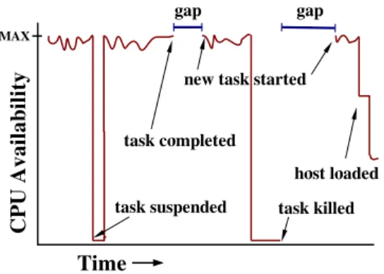
Figure 1 shows an example of the effect of a recruit-ment policy on CPU availability. The task initially uses all the CPU for itself. Then, after some user keyboard/mouse activity, the task gets suspended. (The various causes of task termination to enforce unobtrusiveness include user-level activity such as mouse/keyboard activity, other CPU processes, and disk accesses, or even machine failures, such as a reboot, shutdown or crash.) After the activity subsides and the suspension time expires, the task resumes execution and completes. The worker then uploads the result to the server and downloads a new task; this time is indicated by the interval labelled “gap”. The task be-gins execution then gets suspended and eventually killed, again due to user activity; usually all of the task’s progress is lost as most systems do not have system-level support for checkpointing. Later, after the host becomes available for task execution and the waiting time expires, the task restarts and shortly after beginning execution the host is loaded with other processes but the CPU utilization is be-low the threshold, and so the task continues executing, but only receiving a slice of CPU time.
Figure 1: CPU Availability During Task Execution.
3
The Ideal Resource Trace
An accurate characterization involves obtaining detailed availability traces of the underlying resources. The term “availability” has different meanings in different contexts and must be clearly defined for the problem at hand [4]. In the characterization of these data sets, we distinguished among three types of availability:
1. Host availability. This is a binary value that indi-cates whether a host is reachable, which corresponds to the definition of availability in [5, 1, 4, 11, 28]. Causes of host unavailability include power failure, or a machine shutoff, reboot, or crash.
2. Task execution availability. This is binary value that indicates whether a task can execute on the host or not, according to a desktop grid worker’s recruitment policy. We refer to task execution availability as exec
availability in short. Causes of exec unavailability
include prolonged user keyboard/mouse activity, or a user compute-bound process.
3. CPU availability. This is percentage value that quan-tifies the fraction of the CPU that can be exploited by a desktop grid application, which corresponds to the definition in [3, 9, 29, 12, 30]. Factors that af-fect CPU availability include system and user level compute-intensive processes.
Host unavailability implies exec unavailability, which implies CPU unavailability. Clearly, if a host becomes unavailable (e.g., due to shutdown of the machine), then no new task may begin execution and any executing task would fail. If there is a period of task execution unavail-ability (e.g., due to keyboard/mouse activity), then the desktop grid worker will stop the execution of any task, causing it to fail, and disallow a task to begin execution; as a result of task execution unavailability, the task will observe zero CPU availability.
However, CPU unavailability does not imply exec un-availability. For example, a task could be suspended and therefore have zero CPU availability, but since the task can resume and continue execution, the host is available in terms of task execution. Similarly, exec unavailability does not imply host unavailability. For example, a task could be terminate due to user mouse/keyboard activity, but the host itself could be still up.
Given these definitions of availability, the ideal trace of availability would have the following characteristics:
1. The trace would log CPU availability in terms of the CPU time a real application would receive if it were executing on that host.
2. The trace would record exec availability, in particular when failures occur. From this, one can find the tem-poral structure of availability intervals. We call the interval of time in between two consecutive periods of exec unavailability an availability interval. 3. The trace would determine the cause of the failures
(e.g., mouse/user activity, machine reboot or crash). This would enable statistical modeling (for the pur-pose of prediction, for example) of each particular type of failure.
4. The trace would capture all system overheads. For example, some desktop grid workers run within vir-tual machines [6, 8], and there may be overheads in terms of start-up, system calls, and memory costs.
4
Related Work on Resource
Mea-surements and Modelling
Although a plethora of work has been done on the mea-surement and characterization of host and CPU availabil-ity, there are two main deficiencies of this related research. First, the traces do not capture all causes of task fail-ures (e.g., users’ mouse/keyboard activity), and inferring task failures and the temporal characteristics of availabil-ity from such traces is difficult. Second, the traces may reflect idiosyncrasies of the OS [30, 12] instead of show-ing the true CPU contention for a runnshow-ing task.
In particular, several traces have been obtained that log host availability throughout time. In [7], the authors de-signed a sensor that periodically records each machine’s
uptime from the /procfile system and used this
sen-sor to monitor 83 machines in a student lab. In [24], the authors periodically made RPC calls to rpc.statd, which runs as part of the Network File System (NFS), on 1170 hosts connected to the Internet. A response to the call in-dicated the host was up and a missing response inin-dicated a failure. In [4], a prober runs on the Overnet peer-to-peer file-sharing system looking up host ID’s. A machine with a corresponding ID is available if it responds to the probe; about 2,400 machines were monitored in this fashion. The authors in [11, 28] determine availability by periodically probing IP addresses in a Gnutella system.
Using traces that record only host availability for the purpose of modeling desktop grids is problematic because it is hard to relate uptimes to CPU cycles usable by a desk-top grid application. Several factors can affect an applica-tion’s running time on a desktop grid, which include not only host availability but also CPU load and user activity. Thus, traces that indicate only uptime are of dubious use
for performance modeling of desktop grids or for driving simulations.
Also, there are numerous data sets containing traces of host load or CPU utilization on groups of workstations. Host load is usually measured by taking a moving average of the number of processes in the ready queue maintained by the operating system’s scheduler, whereas CPU utiliza-tion is often measured by the CPU time or clock cycles per time interval received by each process. Since host load is correlated with CPU utilization, we discuss both type of studies in this section.
The CPU availability traces described in [26, 30, 31]
are obtained using the UNIX tools ps and vmstat,
which scan the/proc filesystem to monitor processes.
In particular, the author’s in [26] usedpsto measure CPU
availability on about 13 VAXstationII workstations over a cumulative period of 7 months.
Similarly, the authors in [13] measured host load by periodically using the exponential moving average of the number of processes in the ready queue recorded by the
kernel. In contrast to previous studies on UNIX
sys-tems, the work in [5] measured CPU availability from 3908 Windows NT machines over 18 days by periodically inspecting windows performance counters to determine fractions of cycles used by processes other than the idle process.
None of the trace data sets mentioned above record the various events that would cause application task failures (e.g., keyboard/mouse activity) nor are the data sets im-mune to OS idiosyncrasies. For example, most UNIX process schedulers (the Linux kernel, in particular) give long running processes low priority. So, if a long running process were running on a CPU, a sensor would deter-mine that the CPU is completely unavailable. However, if a desktop grid task had been running on that CPU, the task would have received a sizable chunk of CPU time. Furthermore, processes may have a fixed low priority. Al-though the cause of task failures could be inferred from the data, doing so is not trivial and may not be accurate.
There also been work on measuring the lifetime of pro-cesses run in network of workstations. In [17], the au-thors conduct an empirical study on process lifetimes, and propose a function that fits the measured distribution of lifetimes. Using this model, they determine which pro-cess should be migrated and when. Inferring the temporal structure of availability from this model of process life-times would be difficult because it is not clear how to de-termine the starting point of each process in time in rela-tionship to one another. Moreover, the study did not mon-itor keyboard/mouse activity, which significantly impacts availability intervals [27] in addition to CPU load.
5
Trace Method
We gather traces by submitting measurement tasks to a desktop grid system that are perceived and executed as real tasks. These tasks perform computation and period-ically write their computation rates to file. This method requires that no other desktop grid application be running, and allows us to measure exactly the compute power that a real, compute-bound application would be able to exploit. Our measurement technique differs from previously used methods in that the measurement tasks consume the CPU cycles as a real application would.
During each measurement period, we keep the desk-top grid system fully loaded with requests for our CPU-bound, fixed-time length tasks, most of which were around 10 minutes in length. The desktop grid worker running on each host ensured that these tasks did not interfere with the desktop user and that the tasks were suspended/terminated as necessary; the resource owners were unaware of our measurement activities. Each task of fixed time length consists of an infinite loop that per-forms a mix of integer and floating point operations. A dedicated 1.5GHz Pentium processor can perform 110.7 million such operations per second. Every 10 seconds, a task evaluates how much work it has been able to achieve in the last 10 seconds, and writes this measurement to a file. These files are retrieved by the desktop grid system and are then assembled to construct a time series of CPU availability in terms of the number of operations that were available to the desktop grid application within every 10 second interval.
The main advantage of obtaining traces in this fashion is that the application experiences host and CPU avail-ability exactly as any real desktop grid application would. This method is not susceptible to OS idiosyncrasies be-cause the logging is by done by a CPU-bound task
ac-tually running on the host itself. Also, this approach
captures all the various causes of task failures, includ-ing but not limited to mouse/keyboard activity, operatinclud-ing system failures, and hardware failures, and the resulting trace reflects the temporal structure of availability inter-vals caused by these failures. Moreover, our method takes into account overhead, limitations, and policies of access-ing the resources via the desktop grid infrastructure.
Every measurement method has weaknesses, and our method is certainly not flawless. One weakness compared to the ideal trace data set is that we cannot identify the specific causes of failures, and so we cannot distinguish failures caused by user activity versus power failures, for example. This, in turn, could make stochastic failure pre-diction models more difficult to derive, as one source of failure could skew the distribution of another source.
Nev-ertheless, all types of failures are still subsumed in our traces, in contrast to other studies that often omit many types of desktop failures as described in earlier sections.
Also, the tasks were executed by means of a desktop grid worker, which used a particular recruitment policy. This means that the trace may be biased to the particular worker settings used in the specific deployment. However, with knowledge of these settings, it is straightforward to infer reliably at which points in the trace the bias occurs and thus possible to remove such bias. After removing the bias, one could post-process the traces according to any other CPU-based recruitment policy to determine the corresponding CPU availability. This makes it possible to collect data using our trace method from a desktop grid with one recruitment policy, and then simulate another desktop grid with a different recruitment policy using the same set of traces with minor adjustments.
6
Trace Data Sets
Using the previously described method, we collected data sets from two desktop grids. One of these desk-top grids consisted of deskdesk-top PC’s at the San Diego Su-per Computer Center (SDSC) and ran the commercial
Entropia [10] desktop grid software. We refer to the
data collected from the SDSC environment as the SDSC
trace∗. The other desktop grid consisted of desktop PC’s
at the University of Paris South, and ran the open source XtremWeb [14] desktop grid software. The Xtremweb desktop grid incorporated machines from two different environments. The first environment was a cluster used by a computer science research group for running paral-lel applications and benchmarks, and we refer to the data set collected from this cluster as the LRI trace. The sec-ond environment consisted of desktop PC’s in classrooms used by first-year undergraduates, and we refer to the data set as the DEUG trace. Finally, we obtained the traces first described in [3] which were measured using a dif-ferent trace method and refer to this data set as the UCB
trace†. (We describe this method in Section 5.)
The traces that we obtained from our measurements contain gaps. This is expected as desktop resources be-come unavailable for a variety of reasons, such as the rebooting or powering off of hosts, local processes us-ing 100% of the CPU, the desktop grid worker detectus-ing
∗This data set was first reported previously in [19], but we include
the data set here for completeness and comparison among the other data sets. Several new statistics of the SDSC trace presented here have not been reported previously.
†While the data set was first reported in [3], we present several new
mouse or keyboard activity, or user actively pausing the worker. However, we observe that a very large fraction (≥ 95%) of these gaps are clustered in the 2 minute range. The average small gap length is 35.9 seconds on the En-tropia grid, and 19.5 seconds on the Xtremweb grid.
After careful examination of our traces, we found that these short gaps occur exclusively in between the termi-nation of a task and the beginning of a new task on the same host. We thus conclude that these small gaps do not correspond to actual exec unavailability, but rather are due to the delay of the desktop grid system for starting a new task. In the SDSC grid, the majority of the gaps are spread in the approximate range of 5 to 60 seconds. The sources of this overhead include various system costs of receiving, scheduling, and sending a task as well as an actual built-in limitation that prevents the system from sendbuilt-ing tasks to resources too quickly. That is, the Entropia server en-forces a delay between the time it receives a request from the worker to the time it sends a task to that worker. This is to limit the damaging effect of the “black-hole” prob-lem where a worker does not correctly execute tasks, and instead, repeatedly and frequently sends requests for more tasks from the server. Without the artificial task sending delay, the result of the “black-hole” problem is applica-tions with thousands of tasks that completed instantly but erroneously.
In the XtremWeb grid, the majority of the gaps are between 0 to 5 seconds and 40 to 45 seconds in length. When the Xtremweb worker is available to execute a task, it sends a request to the server. If the server is busy or there is no task to execute, the worker is told to make an-other request after a certain period of time (43 seconds) has expired. This explains the bimodal distribution of gaps length in the XtremWeb system.
Therefore, these small availability gaps observed in both the Entropia and XtremWeb grids would not be ex-perienced by the tasks of a real application, but only in between tasks. Consequently, we eliminated all gaps that were under 2 minutes in our traces by performing linear interpolation. A small portion of the gaps larger than 2 minutes may be also attributed to the server delay and this means that our post-processed traces may be slightly opti-mistic. For a real application, the gaps may be larger due to transfer of input data files necessary for task execution. Such transfer cost could be added to our average small gap length and thus easily included in a performance model.
The weakness of interpolating the relatively small gaps is that this in effect masks short failures less than 2
min-utes in length. Failures due to fast machine reboots
for example could be overlooked using this interpolation method.
6.1
SDSC Trace
The first data set was collected using the Entropia DC-Grid™desktop grid software system deployed at SDSC for a cumulative period of about 1 month across 275 hosts. We conducted measurements during four distinct time periods: from 8/18/03 until 8/22/03, from 9/3/03 un-til 9/17/03, from 9/23/03 to 9/26/03, and from 10/3/03 and 10/6/03 for a total of approximatively 28 days of mea-surements. For our characterization and simulation ex-periments, we use the longest continuous period of trace measurements, which was the two-week period between 9/3/03 - 9/17/03.
Of the 275 hosts, 30 are used by secretaries, 20 are pub-lic hosts that are available in SDSC’s conference rooms, 12 are used by system administrators, and the remaining are used by SDSC staff scientists and researchers. The hosts are all on the same class C network, with most clients having a 10Mbit/sec connection and a few having a 100Mbit/sec connection. All hosts are desktop resources that run different flavors of Windows™. The Entropia server was running on a dual-processor XEON 500MHz machine with 1GB of RAM.
During our experiments, about 200 of the 275 hosts were effectively running the Entropia worker (on the other hosts, the users presumably disabled the worker) and we obtained measurements for these hosts. Their clock rates ranged from 179MHz up to 3.0GHz, with an average of
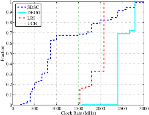
1.19GHz. Figure 2 shows the cumulative distribution
function (CDF) of clock rates. The curve is not continu-ous as for instance no host has a clock rate between 1GHz and 1.45GHz. The curve is also skewed as for instance over 30% of the hosts have clock rates between 797MHz and 863MHz, which represents under 3.5% of the clock rate range.
An interesting feature of the Entropia system is its use of a Virtual Machine (VM) to insulate application tasks from the resources. While this VM technology is critical for security and protection issues, it also makes it possible for fine grain control of an executing task in terms of the resources it uses, such as limiting CPU, memory, and disk usage, and restricting I/O, threads, processes, etc. The design principle is that an application should use as much of the host’s resources as possible while not interfering with local processes. One benefit is that this allows an application to use from 0% to 100% of the CPUs with all possible values in between. It is this CPU availability that we measure. Note that our measurements could easily be post-processed to evaluate a desktop grid system that only allows application tasks to run on host with, say, more than 90% available CPU.
the SDSC data set is that the resolution of the traces is limited to the length of the task. That is, in Entropia, when a task is terminated, the task’s output is lost and as a result, the trace data is lost at the same time. Con-sequently, the unavailability intervals observed in the data set are pessimistic by at most the task length, and the sta-tistical analysis may suffer from some periodicity. How-ever, we believe we can still use the data set for modelling and simulation, and we cross-validate our findings using three other data sets where this limitation in measurement method was removed.
Another weakness is that the interpolation of gaps may have hidden short failures, such as reboots. However, the SDSC system administrations recorded only seven full-system reboots after applying Windows patches during the entire 1-month trace period. (In particular, server reboot at 6PM on 8/18/03, reboot of all desktops at 6:30PM on 8/21, reboot of all desktops on 9/5/03 at 3AM, possible reboot of all desktops if user was prompted on 9/7, server reboot at 6PM on 9/8, reboot of all machines at 11PM on 9/10/03, and reboot of all machines on 9/11/03 (not simul-taneous).) Although this is only a lower bound, we believe that the hosts were rebooted infrequently given that there was usually a single desktop allocated for each user and in that sense were the desktops were dedicated systems. So the phenomenon described in [7] of undergraduates sitting at the desktop rebooting their machines to “clean” the sys-tem of remote users causing high load does not occur.
Finally, because the Entropia system at SDSC was shared with other users, we could only take measurements a few days at a time. By taking traces over consecutive days versus weeks or months, we do not keep track the long-term (e.g., monthly) churn of machines and could lose the long-term temporal structure of availability.
0 500 1000 1500 2000 2500 3000 0 0.1 0.2 0.3 0.4 0.5 0.6 0.7 0.8 0.9 1 Clock Rate (MHz) Fraction SDSC DEUG LRI UCB
Figure 2: Host’s clock rate distribution in each platform
6.2
DEUG and LRI Traces
The second data set was collected using the XtremWeb desktop grid software continuously over about a 1 month period (1/5/05 - 1/30/05) on a total of about 100 hosts at the University of Paris-Sud. In particular, Xtremweb was deployed on a cluster (denoted by LRI) with a total of 40 hosts, and a classroom (denoted by DEUG) with 40 hosts respectively. The LRI cluster is used by the XtremWeb re-search group and other rere-searchers for performance eval-uation and running scientific applications. The DEUG classroom hosts are used by first year students. Typically, the classroom hosts are turned off when not in use. Class-room hosts are turned on on weekends only if there is a class on weekends.
The XtremWeb worker was modified to keep the output of a running task if it had failed, and to return the partial output to the server. This removes any bias due to the failure of a fixed-sized task, and the period of availability logged by the task would be identical to that observed by a real desktop grid application.
Compared to the clock distribution of hosts in the SDSC platform, the hosts in the DEUG and LRI platforms have relatively homogeneous clock rates (see Figure 2). A large mode in the clock rate distribution for the DEUG platform occurs at 2.4GHz, which is also the median; al-most 70% of the hosts have clock rates of 2.4GHz. The clock rates in the DEUG platform range from 1.6GHz to 2.8GHz. In the LRI platform, a mode in the clock rate dis-tribution occurs at about 2GHz, which is also the median; about 65% of the hosts in have clock rates at that speed. The range of clock rates is 1.5GHz to 2GHz.
6.3
UCB Trace
We also obtained an older data set first reported in [3], which used a different measurement method. The traces were collected using a daemon that logged CPU and key-board/mouse activity every 2 seconds over a 46-day pe-riod (2/15/94 - 3/31/94) on 85 hosts. The hosts were used by graduate students the EE/CS department at UC Berkeley. We use the largest continuously measured pe-riod between 2/28/94 and 3/13/94. The traces were post-processed to reflect the availability of the hosts for a desk-top grid application using the following deskdesk-top grid set-tings. A host was considered available for task execution if the CPU average over the past minute was less than 5%, and there had been no keyboard/mouse activity during that time. A recruitment period of 1 minute was used, i.e., a busy host was considered available 1 minute after the ac-tivity subsided. Task suspension was disabled; if a task had been running, it would immediately fail with the first
indication of user activity.
The clock rates of hosts in the UCB platform were all identical, but of extremely slow speeds. In order to make the traces usable in our simulations experiments, we trans-form clock rates of the hosts to a clock rate of 1.5GHz (see Figure 2), which is a modest and reasonable value relative to the clock rates found in the other platforms, and close to the clock rate of host in the LRI platform.
The reason the UCB data set is usable for desktop grid characterization is because the measurement method took into account the primary factors affecting CPU availabil-ity, namely both keyboard/mouse activity and CPU avail-ability. As mentioned previously, the method of deter-mining CPU availability may not be as accurate as our application-level method of submitting real tasks to the desktop grid system. However, given that the desktop grid settings are relatively strict (e.g., a host is considered busy if 5% of the CPU is used), we believe that the result of post-processing is most likely accurate. The one weak-ness of this data set is that it more than 10 years old, and host usage patterns might have changed during that time. We use this data set to show that in fact many character-istics of desktop grids have remained constant over the years. Note that the UCB trace is the only previously ex-isting data set that tracked user mouse/keyboard activity, which is why it is usable for desktop grid characterization, modelling, and simulations.
7
Characterization of Exec
Avail-ability
In this section, we characterize in detail exec availability and in our discussion, the term availability will denote exec availability unless noted otherwise. We report and discuss aggregate statistics over all hosts in each platform, and when relevant, we also describe per host statistics.
7.1
Number of Hosts Available Over Time
We observed the total number of hosts available over time to determine at which times during the week and during each day machines are the most volatile. This can be use-ful for determining periods of interest when testing vari-ous scheduling heuristics, for example.
With the exception of the LRI trace, we observe a diur-nal cycle of volatility beginning in general during week-day business hours. That is, during the business hours, the variance in the number of machines over time is relatively high, and during non-business hours, the number becomes relatively stable. In the case of UCB and SDSC trace,
the number of machines usually decreases during these business hours, whereas in the DEUG trace, the number of machines can increase or decrease. This difference in trends can be explained culturally. Most machines in en-terprise environments in the U.S. tend to be powered on through the day, and so any fluctuation in the number hosts are usually downward fluctuations. In contrast, in Europe, machines are often powered off when not in use during business hours (to save power or to reduce fire haz-ards, for example), and as a result, the fluctuations can be upward.
Given that students and staff scientists form the major-ity of the user base at SDSC and UCB, we believe the cause of volatility during business hours is primarily key-board/mouse activity by the user or keyboard, or perhaps short compilations of programming code rather than long computations, which can be run on clusters or supercom-puters at SDSC or UCB. This is supported by observations in other similar CPU availability studies [27, 26]. In the DEUG platform, the volatility is most likely due to ma-chines being powered on and off, in addition to interactive desktop activity.
The number of hosts in the LRI trace does not follow any diurnal cycle. This trend can be explained by the user base of the cluster, i.e., computer science researchers that submit long running batch jobs to the cluster. The result is that hosts tend to be unavailable in groups at a time, which is reflected by the large drop in host number on 1/10/05. Moreover, there is little interactive use of the cluster, and so the number of hosts over time remains rel-atively constant. Also, the LRI cluster (with the exception of a handful of nodes, possibly front-end nodes) is turned off on weekends, which explains the drop on Sunday and Saturday.
We refer to the daily time period during which the set of hosts is most volatile as business hours. After close examination of the number of hosts over time, we deter-mine that times delimiting business hours for the SDSC, DEUG, and UCB platforms are 9AM-5PM, 6AM-6PM, and 10AM-5PM respectively. Regarding the LRI plat-form, we make no distinction between non-business hours and business hours.
7.2
Temporal Structure of Availability
The successful completion of a task is directly related to the size of availability intervals, i.e., intervals between two consecutive periods of unavailability. Here we show the distributions of various types of availability intervals for each platform, which characterize its volatility.
inter-0 2 4 6 8 10 0 0.1 0.2 0.3 0.4 0.5 0.6 0.7 0.8 0.9 1
Interval length (hours)
Cumulative percentage SDSC mean: 2.0372 DEUG mean: 0.47727 LRI mean: 23.535 UCB mean: 0.16663 SDSC DEUG LRI UCB
(a) Business hours.
0 2 4 6 8 10 0 0.1 0.2 0.3 0.4 0.5 0.6 0.7 0.8 0.9 1
Interval length (hours)
Cumulative percentage SDSC mean: 10.2327 DEUG mean: 17.4239 UCB mean: 0.82374 SDSC DEUG UCB (b) Non-business hours.
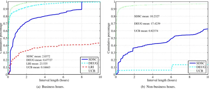
Figure 3: Cumulative distribution of the length of availability intervals in terms of time for business hours and non-business hours.
vals in terms of hours over all hosts in each platform. Fig-ures 3(a) and 3(b) show the intervals for business hours and non-business hours respectively where the business hours for each platform are as defined in Section 7.1. In the case a host is available continuously during the entire business hour or non-business hour period, we truncate the intervals at the beginning and end of the respective period. We do not plot availability intervals for LRI dur-ing non-business hours, i.e., the weekend, because most of the machines were turned off then.
Comparing the interval lengths from business hours to non-business hours, we observe expectedly that the lengths tend to be much longer on weekends (at least 5 times longer). For business hours, we observe that the UCB platform tends to have the shortest lengths of avail-ability (µ '10 minutes), whereas DEUG, SDSC have rel-atively longer lengths of availability (µ 'half hour, two hours, respectively). The LRI platform by far exhibits the longest lengths (µ '23.5 hours).
The UCB platform has the shortest length most likely because the CPU threshold of 5% is relatively low. The authors in [26] observed that system daemons can often cause load up to 25%, and so this could potentially in-crease the frequency of availability interruptions. In addi-tion, the UCB platform was used interactively by students, and often keyboard/mouse activity can cause momentary short bursts of 100% CPU activity. Since the hosts in the DEUG and SDSC platforms also were used interactively, the intervals are also relatively short. We surmise that the long intervals of the LRI platform are result of the
clus-ter’s workload, which often consists of periods of high activity and followed by low activity. So, when the clus-ter is not in use, the nodes tend to be available for longer periods of time.
In summary, the lower the CPU threshold, the shorter the availability intervals. Availability intervals tend to be shorter in interactive environments, and intervals tend to be longer during business hours than non-business hours. While this data is interesting for applications that re-quire hosts to be reachable for a given period of time (e.g., content distribution) and could be used to confirm and ex-tend some of the work in [5, 4, 11, 28], it is less relevant to other problems, such as scheduling compute-intensive tasks. Indeed, from the perspective of a compute-bound application, a 1GHz host that is available for 2 hours with average 80% CPU availability is less attractive than, say, a 2GHz host that is available for 1 hour with average 100% CPU availability.
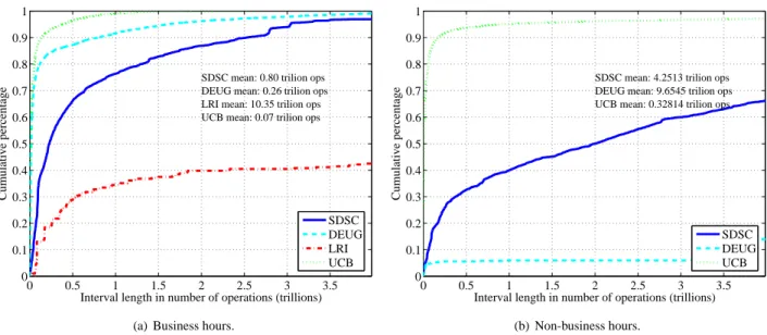
By contrast, Figure 4 plots the cumulative distribution of the availability intervals, both for business hours and non-business hours, but in terms of the number of opera-tions performed. In other words, these are intervals during which a desktop grid application task may be suspended, but does not fail. So instead of showing availability inter-val durations, the x-axis shows the number of operations that can be performed during the interval, which is com-puted using our measured CPU availability. This quanti-fies directly the performance that an application, factoring in the heterogeneity of hosts. Other major trends in the data are as expected with hosts and CPUs are more
fre-0 0.5 1 1.5 2 2.5 3 3.5 0 0.1 0.2 0.3 0.4 0.5 0.6 0.7 0.8 0.9 1
Interval length in number of operations (trillions)
Cumulative percentage
SDSC mean: 0.80 trilion ops DEUG mean: 0.26 trilion ops LRI mean: 10.35 trilion ops UCB mean: 0.07 trilion ops
SDSC DEUG LRI UCB
(a) Business hours.
0 0.5 1 1.5 2 2.5 3 3.5 0 0.1 0.2 0.3 0.4 0.5 0.6 0.7 0.8 0.9 1
Interval length in number of operations (trillions)
Cumulative percentage
SDSC mean: 4.2513 trilion ops DEUG mean: 9.6545 trilion ops UCB mean: 0.32814 trilion ops
SDSC DEUG UCB
(b) Non-business hours.
Figure 4: Cumulative distribution of the length of availability intervals in terms of operations for business hours and non-business hours.
quently available during business hours than non-business hours. This empirical data enables us to quantify task fail-ure rates and develop a performance model (see [19] for an example with the SDSC data set).
7.3
Temporal Structure of Unavailability
It useful also to know how long a host is typically un-available, i.e., unable to execute a task (for example, when scheduling an application). Given two hosts with identi-cal availability interval lengths, one would prefer the host with smaller unavailability intervals. Using availability and unavailability interval data, one can predict whether a host has a high chance of completing a task by a certain time, for example.
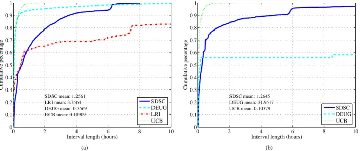
Figure 5 shows the CDF of the length of unavailabil-ity intervals in terms of hours during business hours and non-business hours for each platform. Note that although a platform may exhibit a heavy-tailed distribution, it does not necessarily mean that the platform is generally less available. (We describe CPU availability later in Sec-tion 8.1.)
We observe several distinct trends for each platform. First, for the SDSC, platform we notice that the unavail-ability intervals are longer during business hours than non-business hours. This can be explained by the fact that on weekends patches were installed and backups were done, and several short unavailability intervals could re-sult if these were done as a batch. Second, for the DEUG platform, we found unavailability intervals tend to be
much shorter on business hours (µ =∼20 min ) versus
non-business hours (µ =∼32 hours ). The explanation
is that many of the machines are turned off at night or on weekends, resulting in long periods of unavailability. The fact that during non-business hours more than 50% of DEUG’s unavailability intervals are less than a half hour in length could be explained by a few machines still be-ing used interactively durbe-ing non-business hours. Third, for the LRI platform, we notice that 60% of unavailability intervals are less than 1 hour in length. This could be due to the fact that most jobs submitted to clusters or MPP’s tend to be quite short in length [25]. Lastly, for the UCB platform, the CDF of unavailability intervals appears sim-ilar. We believe this is because the platform’s user base are students and while the number of machines in use during business hours versus non-business hours is less, the pattern in which the students use the machines is the same (i.e., using the keyboard/mouse and running short processes), resulting in nearly identical distributions.
7.4
Task Failure Rates
Based on our characterization of the temporal structure of resource availability, it is possible to derive the ex-pected task failure rate, that is the probability that a host will become unavailable before a task completes, from the distribution of number of operations performed in be-tween periods of unavailability (from the data shown in Figure 4(a)) based on random incidence. To calculate the failure rate, we choose hundreds of thousands of
ran-0 2 4 6 8 10 0 0.1 0.2 0.3 0.4 0.5 0.6 0.7 0.8 0.9 1
Interval length (hours)
Cumulative pecentage SDSC mean: 1.2561 LRI mean: 3.7564 DEUG mean: 0.3569 UCB mean: 0.11909 SDSC DEUG LRI UCB (a) 0 2 4 6 8 10 0 0.1 0.2 0.3 0.4 0.5 0.6 0.7 0.8 0.9 1
Interval length (hours)
Cumulative pecentage SDSC mean: 1.2645 DEUG mean: 31.9517 UCB mean: 0.10379 SDSC DEUG UCB (b)
Figure 5: Unavailability intervals in terms of hours
dom points during periods of exec availability in traces. At each point, we determine whether a task of a given size (i.e., number of operations) would run to completion given that the host was available for task execution. If so, we count this trial as a success; otherwise, we count the trial as a failure. We do not count tasks that are started during periods of exec unavailability.
Figure 6(a) shows the expected task failure rates com-puted for business hours for each platform. Also, the least squares line for each platform is superimposed with a dotted magenta line, and the correlation coefficient ρ is shown. For illustration purposes, the x-axis shows task sizes not in number of operations, but in execution time on a dedicated 1.5GHz host, from 5 minutes up to almost 7 hours.
The expected task failure rate is strongly dependent on the task lengths. (The weekends show similar linear trends, albeit the failure rates are lower.) The platforms with failure rates from lowest to highest are LRI, SDSC, DEUG, and UCB, which agrees with the ordering of each platform shown in Figure 4(a). It appears that in all plat-forms the task failure rate increases with task size and that the increase is almost linear; the lowest correlation coeffi-cient is 0.98, indicating that there exists a strong linear re-lationship between task size and failure rate. By using the least squares fit, we can define a closed-form model of the aggregate performance attainable by a high-throughput application on the corresponding desktop grid (see [19] for an example with the SDSC data set). Note, however, that the task failure rate for larger tasks will eventually plateau as it approaches one.
While Figure 6(a) shows the aggregate task failure rate of the system, Figure 6(b) shows the cumulative distribu-tion of the failure rate per host in each platform, using particular task size of 35 minutes on a dedicated 1.5GHz host. The heavier the tail, the more volatile the hosts in the platform. Overall, the distributions appears quite skewed. That is, a majority of the hosts are relatively sta-ble. For example, with the DEUG platform, about 75% of the hosts have failure rates of 20% or less. The UCB platform is the least skewed, but even so, over 70% of the hosts have failure rates of 40% or less. The fact that most hosts have relatively low failure rates can affect schedul-ing for example tremendously as shown in [18].
Surprisingly, in Figure 6(a), SDSC has lower task fail-ure rates than UCB, yet in Figfail-ure 6(b), SDSC has a larger fraction of hosts with failure rates 20% or less compared to UCB. The discrepancy can be explained by the fact that UCB still has a larger fraction of hosts with failure rates 40% or more than SDSC; after averaging, SDSC has lower failure rates.
7.5
Correlation of Availability Between
Hosts
An assumption that permeates fault tolerance research in large scale systems is that resource failure rates can be modelled with independent and identical probability
distributions (i.i.d). Moreover, a number of analytical
studies in desktop grids assume that exec availability is i.i.d. [21, 20, 16] to simplify probability calculations. We investigate the validity of such assumptions with respect
0 50 100 150 200 250 300 350 0 0.1 0.2 0.3 0.4 0.5 0.6 0.7 0.8 0.9 1
Task size (minutes on a 1.5GHz machine)
Fraction of Tasks Failed
SDSC ρ: 0.99231 DEUG ρ: 0.98812 LRI ρ: 0.99934 UCB ρ: 0.98223 SDSC DEUG LRI UCB (a) Aggregate 0 0.2 0.4 0.6 0.8 1 0 0.1 0.2 0.3 0.4 0.5 0.6 0.7 0.8 0.9 1 Failure Rate Cumulative Fraction SDSC DEUG LRI UCB
(b) Per host for 35 minute tasks
Figure 6: Task failure rates during business hours
to exec availability in desktop grid systems.
First, we studied the independence of exec availability across hosts by calculating the correlation of exec avail-ability between pairs of hosts. Specifically, we compared the availability for each pair of hosts by adding 1 if both machines were available or both machines were unavail-able, and subtracting 1 if one host was available and the other one was not. This method was used by the authors in [5] to study the correlation of availability among thou-sands of hosts at Microsoft.
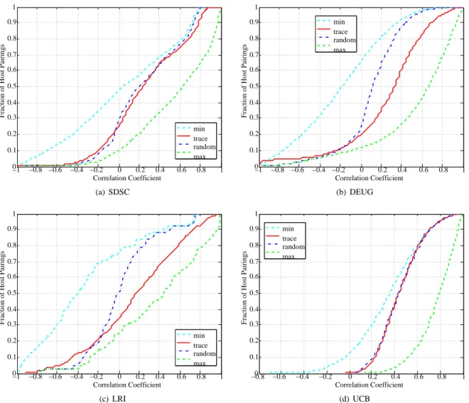
Figure 7 shows the cumulative fraction of hosts pairs that are below a particular correlation coefficient. The line labelled “trace” in the legend indicates correlation calcu-lated according to the traces. The line labelled “min” indi-cates the minimum possible correlation given the percent of time each machine is available, and likewise for the line labelled “max”.
In Figure 7b corresponding to the DEUG platform, the point (0.4, 0.6) means that for 60% of all possible host pairing, the percent of time that the two host’s availabil-ity “matched” was 40% or less than the time the hosts’ availability “mismatched”. The difference between points (0.4, 0.6) and (0.66, 0.6) means that for the same frac-tion of host pairings, there is 26% more “matching” possi-ble among the hosts. The difference between points (-0.2, 0.1) and (-0.8, 0.1) indicates for 10% of the host pairings, there could have been at most 60% more “mismatching” availability. The point (-0.4, 0.05) means that for 5% of the host pairings, the availability “mismatched” 40% or more of the time more often than “matched”.
Overall, we can see that in all the platforms at least
60% of the host pairings had positive correlation, which indicates that a host is often available or unavailable when another host is available or unavailable respectively. How-ever, Figures 7(a) and 7(d) also show that this correla-tion is due to the fact that most hosts are usually avail-able (when combined with the fact that 80% of the time, hosts have CPU availability of 80% or higher), which is reflected by how closely the trace line follows the ran-dom line in the figure. That is, if two host are available (or unavailable) most of the time, they are more likely to be available (or unavailable) at the same, even randomly. As a result, the correlation observed in the traces would in fact occur randomly because the hosts have such high availability. This in turn gives strong evidence (although not completely sufficient) that the exec availabilities of hosts in the SDSC and UCB platforms are independent.
We believe the high likelihood of independence of exec availability in the SDSC and DEUG traces is primarily due to the user base of the hosts. As mentioned previ-ously, the user base of the SDSC consisted primarily of re-search scientists and administrators who we believe used the Windows hosts primarily for word processing, surfing the Internet, and other tasks that did not directly affect the availability of other hosts. Similarly, for the UCB plat-form, we believe the students used the host primarily for short durations, which is evident by the short availability intervals. So, because the primary factors causing host un-availability, i.e., user processes and keyboard/mouse ac-tivity, are often independent from one machine to another in desktop environments, we observe that exec availability in desktop grids is often not significantly correlated.
−1 −0.8 −0.6 −0.4 −0.2 0 0.2 0.4 0.6 0.8 1 0 0.1 0.2 0.3 0.4 0.5 0.6 0.7 0.8 0.9 1 Correlation Coefficient
Fraction of Host Pairings
min trace random max (a) SDSC −1 −0.8 −0.6 −0.4 −0.2 0 0.2 0.4 0.6 0.8 1 0 0.1 0.2 0.3 0.4 0.5 0.6 0.7 0.8 0.9 1 Correlation Coefficient
Fraction of Host Pairings
min trace random max (b) DEUG −1 −0.8 −0.6 −0.4 −0.2 0 0.2 0.4 0.6 0.8 1 0 0.1 0.2 0.3 0.4 0.5 0.6 0.7 0.8 0.9 1 Correlation Coefficient
Fraction of Host Pairings
min trace random max (c) LRI −0.80 −0.6 −0.4 −0.2 0 0.2 0.4 0.6 0.8 1 0.1 0.2 0.3 0.4 0.5 0.6 0.7 0.8 0.9 1 Correlation Coefficient
Fraction of Host Pairings
min trace random max
(d) UCB
Figure 7: Correlation of availability.
On the other hand, Figures 7(b) and 7(c) show differ-ent trends where the line corresponding to the trace dif-fers significantly with respect to correlation (as much as 20%) from the line corresponding to random correlation. The weak correlation of the DEUG trace is due to the par-ticular configuration of the classroom machines. These machines had wake-on-LAN enabled Ethernet adapters, which allowed the machines to be turned on remotely. The system administrators had configured these machines to “wake” every hour if they had been turned off by a user. Since most machines are turned off when not in use, many machines were awakened at the same time, resulting in the weak correlation of availability. We believe that this wake-on-LAN configuration is specific to the configura-tion of the machines in DEUG, and that in general, ma-chine availability is independent in desktop grids where
keyboard/mouse activity is high.
Hosts in the LRI platform also shows significant cor-relation relative to random. This behavior is expected as batch jobs submitted to the cluster tend to consume a large number of nodes simultaneously, and consequently, the nodes are unavailable for desktop grid task execution at the same times.
The independence result is supported by the host avail-ability study performed at Microsoft reported in [5]. In this study, the authors monitored the uptimes of about 50,000 desktops machines over a 1 week period, and found that the correlation of host availability matched random correlation. Host unavailability implies exec availability, and so our measurements subsume host un-availability in addition to the primary factors that cause exec unavailability, i.e., CPU load and keyboard/mouse
activity. We show that exec availability between hosts is not significantly correlated when taking into the effects of CPU load, keyboard/mouse activity, in addition to host availability.
Another difference between our study and the Mi-crosoft study is that the MiMi-crosoft study analyzed the cor-relation of the 50,000 machines as a whole and did not separate the 50,000 desktop machines into departmental groups (such as hosts used by administrators, software de-velopment groups, and management, for example). So it is possible that some correlation within each group was hidden. In contrast, the groups of host that we analyzed had a relatively homogeneous user base, and our result is stronger in the sense that we rule out the possibility of correlation among hosts with heterogeneous user bases.
Other studies of host availability have in fact shown correlation of host failures [2] due to power outages or network switches. While such failures can clearly affect application execution, we do not believe these types of failures are the dominant cause of task failures for desk-top grid applications. Instead, the most common cause of task failures is due to either high CPU load or key-board/mouse activity [27], and our study directly takes into account these factors affect exec availability in con-trast to the other studies. So although host availability may be correlated, this correlation is significantly weak-ened by the major causes of exec unavailability. The as-sumption of host independence, which we give evidence for, can be used to simplify the (probabilistic) failure anal-ysis of these platforms.
7.6
Correlation of Availability with Host
Clock Rates
We hypothesized that a host’s clock rate would be a good
indicator of host performance. Intuitively, host speed
could be correlated with a number of other machine char-acteristics. For example, the faster a host’s clock rate is, the faster it should complete a task, and the lower the fail-ure rate should be. Or the faster a host’s clock rate is, the more often a user will be using that particular host, and the less available the host will be. Surprisingly, host speed is not as correlated with these factors as we first believed.
Table 1 shows the correlation of clock rate with various measures of host availability for the SDSC trace. (Be-cause the clock rates in the other platforms were roughly uniform, we could not calculate the correlation.) Since clock rates often increase exponentially throughout time, we also compute the correlation of the log of clock rates with the other factors. We compute the correlation be-tween clock rate and the mean time per availability
in-terval to capture the relationship between clock rate the temporal structure of availability . However, it could be the case that a host with very small availability intervals is available most of the time. So, we also compute the cor-relation between clock rate and percent of time each host is unavailable . We find that there is little correlation be-tween the clock rate and mean length of CPU availability intervals in terms of time (see rows 1 and 2 in Table 1), or percent of the time the host is unavailable (see rows 3 and 4). We explain this by the fact that many desktops for most of the time are being used for intermittent and brief tasks, for example for word processing, and so even machines with relatively low clock rates can have high unavailabil-ity (for example due to frequent mouse/keyboard activ-ity), which results in availability similar to faster hosts. Moreover, the majority of desktops are distributed in of-fice rooms. So desktop users do not always have a choice of choosing a faster desktop to use.
What matters more to an application than the time per interval is the operations per interval, how it affects the task failure rate, and whether it is related to the clock rate of the host. We compute the correlation between clock rate and CPU availability in terms of the mean operations per interval and failure rate for a 15 minute task. There is only weak positive correlation between clock rate and the mean number of operations per interval (see rows 5 and 6), and weak negative correlation between the clock rate and failure rate (see rows 7 and 8). Any possibility of strong correlation would have been weakened by the ran-domness of user activity. Nevertheless, the factors are not independent of clock rate because hosts with faster clock rates tend to have more operations per availability inter-val, thus increasing the chance that a task will complete during that interval.
Furthermore, in rows 9 and 10 of Table 1, we see the relationship between clock rate and rate of successful task completion within a certain amount of time. In particular, rows 9 and 10 show the fairly strong positive correlation between clock rate and the probability that a task com-pletes in 15 minutes or less. The size of the task is 15 minutes when executed on a dedicated 1.5GHz. (We also computed the correlation for other task sizes and found similar correlation coefficients). Clearly, whether a task completes in a certain amount of time is related to clock rate. However, this relationship is slightly weakened due to the randomness of exec unavailability, as unavailability could cause a task executing on a relatively fast host to fail. One implication of this correlation shown in rows 5-10 is that a scheduling heuristic based on using host clock rates for task assignment may be effective, and this is in-vestigated further in [18].
X Y ρ
clock rate mean availability interval length (time) -0.0174
log (clock rate) mean availability interval length (time) -0.0311
clock rate % of time unavailable 0.1106
log (clock rate) % of time unavailable 0.1178
clock rate mean availability interval length (ops) 0.5585
log (clock rate) mean availability interval length (ops) 0.5196
clock rate task failure rate (15 minute task) -0.2489
log (clock rate) task failure rate (15 minute task) -0.2728
clock rate P(complete 15 min task in 15 min) 0.859
log (clock rate) P(complete 15 min task in 15 min) 0.792
Table 1: Correlation of host clock rate and other machine characteristics during business hours for the SDSC trace
Task size Failure rate ρ
5 0.063 -0.2053 10 0.097 -0.2482 15 0.132 -0.2489 20 0.155 -0.2624 25 0.177 -0.2739 30 0.197 -0.280 35 0.220 -0.2650
Table 2: Correlation of host clock rate and failure rate during business hours. Task size is in term of minutes on a dedicated 1.5GHz host.
The correlation between host clock rate and task fail-ure rate should increase with task size (until all hosts have very high failure rates close to 1). Short tasks that have a very low mean failure rate (near zero) over all hosts will naturally have low correlation. As the task size in-creases, the failure rate will be more correlated with clock rates since in general the faster hosts will be able to fin-ish the tasks sooner. Table 2 shows the correlation coeffi-cient between clock rate and failure rate for different task sizes. There is only weak negative correlation between host speed and task failure rate, and it increases in general with the task size as expected. Again, we believe the weak correlation is partly due to the randomness of keyboard and mouse activity on each machine. One consequence of this result with respect to scheduling is that the larger the task size, the more important it is to schedule the tasks on hosts with faster clock rates.
8
Characterization of CPU
Avail-ability
While the temporal structure of availability directly im-pacts task execution, it is also useful to observe the CPU availability of the entire system for understanding how the temporal structure of availability affects system per-formance as a whole, and how the CPU availability per availability interval fluctuates if at all. That is, aggregate CPU availability puts availability and unavailability inter-vals into perspective, capturing the effect of both types of intervals on the compute power of system as statistics of either availability intervals or unavailability intervals do not necessarily reflect the characteristics of the other.
8.1
Aggregate CPU Availability
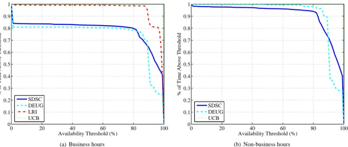
An estimate of the computational power (i.e., number of cycles) that can be delivered to a desktop grid applica-tion is given by an aggregate measure of CPU availability. For each data point in our measurements (over all hosts), we computed how often CPU availability is above a given threshold for both business hours and non-business hours on each platform. Figures 8(a) and 8(b) plot the frequency of CPU availability being over a threshold for threshold
values from from 0% to 100%: the data point(x, y) means
that y% of the time CPU availability is over x%. For instance, the graphs show that CPU availability for the SDSC platform is over 80% about 80% of the time during business hours, and 95% of the time during non-business hours.
In general, CPU availability tends to be higher during business hours than non-business hours. For example, on business hours, the SDSC and DEUG platforms have zero CPU availability about 15% of the time, whereas during
0 20 40 60 80 100 0 0.1 0.2 0.3 0.4 0.5 0.6 0.7 0.8 0.9 1 Availability Threshold (%)
% of Time Above Threshold
SDSC DEUG LRI UCB
(a) Business hours
0 20 40 60 80 100 0 0.1 0.2 0.3 0.4 0.5 0.6 0.7 0.8 0.9 1 Availability Threshold (%)
% of Time Above Threshold
SDSC DEUG UCB
(b) Non-business hours
Figure 8: Percentage of time when CPU availability is above a given threshold, over all hosts, for business hours and non-business hours.
business hours, the same hosts in the same platforms al-most always have CPU availability greater or equal to zero. During business hours, we observe that SDSC and DEUG have an initial drop from a threshold of 0% to 1%. We believe the CPU unavailability indicated by this drop is primarily due to exec unavailability cause by user ac-tivity/process on the hosts in the system. Other causes of CPU unavailability include the suspension of the desktop grid task or brief bursts of CPU unavailability that are not long enough to cause load on the machine to go below the CPU threshold. The exceptions are the UCB and LRI platforms that shows no such drop. The UCB platform is level from 0 to 1% because the worker’s CPU threshold is relatively stringent (5%), resulting in common but very brief unavailability intervals which have little impact on the overall CPU availability of the system. One reason that the LRI plot is relatively virtually constant between 0 and 1% is that the cluster is lightly loaded so most host’s CPU’s are available most of the time.
After this initial drop between threshold of 0 and 1%, the curves remain almost constant until the respective CPU threshold is reached. The levelness is an artifact of the worker’s CPU threshold used to determine when to terminate a task. That is, the only reason our com-pute bound task (with little and constant I/O) would have a CPU availability less than 100% is if there were other processes of other users running on the system. When CPU usage of the host’s user(s) goes above the worker’s CPU threshold, the task is terminated, resulting in the virtually constant line from the 1% threshold to (100%
- worker’s CPU threshold). (Note in the case of UCB, we assume that either the host’s CPU is completely avail-able or unavailavail-able, which is valid given that the worker’s CPU threshold was 5%.) The reason that the curves are not completely constant during this range is possibly be-cause of system processes that briefly use the CPU, but not long enough to increase the moving average of host load to cause the desktop grid task to be terminated.
Between the threshold of (100% - worker’s CPU threshold) and 100%, most of the curves have a downward slope. Again, the reason this slope occurs, is that system processes (which often use 25% of the CPU [22]) are run-ning simultaneously. On average for the SDSC platform, CPU’s are completely unavailable 19% of the time dur-ing weekdays and 3% of the cases durdur-ing weekends. We also note that both curves are relatively flat for CPU avail-ability between 1% and 80%, denoting that hosts rarely exhibit availabilities in that range.
Other studies have obtained similar data about aggre-gate CPU availability in desktop grids [10, 23]. While such characterizations make it possible to obtain coarse estimates of the power of the desktop grid, it is difficult to related them directly to what a desktop grid application can hope to achieve. In particular, the understanding of host availability patterns, that is the statistical properties of the duration of time intervals during which an applica-tion can use a host, and a characterizaapplica-tion of how much power that host delivers during these time intervals, are key to obtaining quantitative measures of the utility of a platform to an applications. We develop such a
character-ization in [19].
8.2
Per Host CPU Availability
While aggregate CPU availability statistics reflect the overall availability of the system, it is possible some hosts are less available than others. We investigate CPU avail-ability per host to reveal any potential imbalance.
In the SDSC trace, we observe heavy imbalance in terms of CPU unavailability. Moreover, it appears that CPU availability does not always increase with host clock rate as several of the slowest 50% of the hosts have CPU unavailability greater than or equal to 40% of the time. In the LRI trace, we see that the system is relatively under-utilized as few of the hosts in the LRI cluster have CPU unavailability greater than 5%. In the UCB trace, we ob-serve that the system is also underutilized as none of the hosts have CPU unavailability greater than 5% of the time; we believe this is a result of the system’s low CPU thresh-old. In summary, the CPU availability does not show strong correlation with clock rate, which is reaffirmed by Table 2, and the amount of unavailability is strongly de-pendent on the user base and worker’s criteria for idleness. One implication of this result is that simple probabilistic models of desktop grid systems (such as those described in [16, 20]) that assume hosts have constant frequencies of unavailability and constant failure rates are insufficient for modelling these complex systems.
9
Summary and Future Work
We described a simple trace method that measured CPU availability in a way that reflects the same CPU availabil-ity that could be experienced by real application. We used this method to gather data sets on three platforms with distinct clock rate distributions and user types. In addi-tion, we obtained a fourth data set gathered earlier by the authors in [3]. Then, we derived several useful statistics regarding exec availability and CPU availability for each system as a whole and individual hosts.
The findings of our characterization study can be sum-marized as follows. First, we found that even in the most volatile platform with the strictest host recruitment pol-icy availability intervals tend to be 10 minutes in length or greater, while the mean length over all platforms with interactive users was about 2.6 hours. To apply this result, an application developer could ensure that tasks are about 10 minutes in length to utilize effectively the majority of availability intervals for task completion.
Second, we found that task failure rates on each system were correlated with the task size, and so task failure rate
can be approximated as a linear function of task size. This in turn allowed us to construct a closed-form performance model of the system, which we describe in future work.
Third, we observed that on platforms with interactive users, exec availability tends to be independent across
hosts. However, this independence is affected
signif-icantly by the configuration of the hosts; for example wake-on-LAN enabled Ethernet adapters can cause cor-related availability among hosts. Also, in platforms used to run batch jobs, availability is significantly correlated.
Fourth, the availability interval lengths in terms of time are not correlated with clock rates nor is the percentage of time a host is unavailable. This means that hosts with faster clock rates are not necessarily used more often. Nevertheless, interval lengths in terms of operations and task failure rates are correlated with clock rates. This indi-cates that the selecting resources according to clock rates may be beneficial.
Finally, we studied the CPU availability of the re-sources. We found that because of the recruitment poli-cies of each worker, the CPU availability of the hosts are either above 80% or zero. Regarding the CPU availability per host, there is wide variation of availability from host to host, especially in the platforms with interactive users. As a result, even in platforms with hosts of identical clock rates, there is significant heterogeneity in terms of the per-formance of each host with respect to the application.
For future work, we plan on obtaining traces on Inter-net desktop grid environments using BOINC [15], for ex-ample. When then hope to extend our characterization to Internet desktop grids environments, and compare and contrast the results to enterprise environments. Also, we will characterize other host features, such as memory and network connectivity.
Acknowledgments
We gratefully acknowledge Kyung Ryu and Amin Vahdat for providing the UCB trace data set and documentation.
References
[1] A. Acharya, G. Edjlali, and J. Saltz. The Utility of Exploiting Idle Workstations for Parallel Computa-tion. In Proceedings of the 1997 ACM
SIGMET-RICS International Conference on Measurement and Modeling of Computer Systems, pages 225–234,