Using the Dual-Criteria Methods to Supplement Visual Inspection: An Analysis of Nonsimulated Data
Marc J. Lanovaz, Sarah C. Huxley, and Marie-Michèle Dufour Université de Montréal
Author Note
This research project was supported in part by a grant from the Canadian Institutes of Health Research (# MOP – 136895) and a salary award from the Fonds de Recherche du Québec – Santé (# 30827) to the first author.
Correspondence concerning this article should be addressed to Marc J. Lanovaz, École de Psychoéducation, Université de Montréal, C.P. 6128, succursale Centre-Ville, Montreal, QC, Canada, H3C 3J7.
Email: marc.lanovaz@umontreal.ca
This is the peer reviewed version of the following article:
Lanovaz, M. J., Huxley, S. C., & Dufour, M.-M. (2017). Using the dual-criteria methods to supplement visual inspection: An analysis of nonsimulated data. Journal of Applied Behavior Analysis, 50, 662-667.
which has been published in final form at https://doi.org/10.1002/jaba.394. This article may be used for non-commercial purposes in accordance with Wiley Terms and Conditions for Self-Archiving.
Abstract
The purpose of our study was to examine the probability of observing false positives in non-simulated data using the dual-criteria methods. We extracted data from published studies to produce a series of 16,927 datasets and then assessed the proportion of false positives for various phase lengths. Our results indicate that collecting at least 3 data points in the first phase (Phase A) and at least 5 data points in the second phase (Phase B) is generally sufficient to produce acceptable levels of false positives.
Using the Dual-Criteria Methods to Supplement Visual Inspection: An Analysis of Nonsimulated Data
In their seminal paper, Baer, Wolf, and Risley (1968) included the analytic dimension as one of the defining features of the science of applied behavior analysis. This dimension involves producing a convincing demonstration that an independent variable (e.g., treatment), and not some other confounding variable, is generating a behavior change. Behavior analysts have widely adopted the use of single-case experimental designs to analyze the effects of their treatments in both research and practice. Although visual inspection remains the norm in the analysis of single-case experimental designs (e.g., Bourret & Pietras, 2014; Fahmie & Hanley, 2008), researchers have shown that interrater agreement between visual analysts is not always strong (Ninci, Vannest, Willson, & Zhang, 2015).
To address this issue, Fisher, Kelley, and Lomas (2003) developed the dual-criteria (DC) and conservative dual-criteria (CDC) methods, which involve using structured criteria to
supplement visual analysis of AB, reversal, and multiple baseline designs. Specifically, the DC method involves (a) tracing a continuation of the mean and trend lines from the first phase onto the second phase, (b) counting the number of points that fall above or below both lines in the second phase, and (c) comparing this number of points with a cut-off value based on the binomial distribution. The CDC method is the same except that the mean and trend lines are raised or lowered by 0.25 standard deviations. Using simulated data, Fisher et al. showed that both methods were generally adequate to supplement visual analysis of single-case graphs. Although the DC method was more powerful, the CDC method generally produced more acceptable proportions of false positives (α < .05).
One limitation of the previous study is that simulated datasets may not fully capture patterns of behavior typically encountered in applied work. The randomness may not perfectly mimic the effects of confounding variables already present in the environment such as events occurring outside treatment sessions, physiological and environmental motivating operations, and maturation. Thus, we sought to extend Fisher et al.’s study by examining the probability of a false positive result when the DC and CDC methods were used to interpret data extracted from published studies.
Method
Previously published datasets that include extended baseline phases (i.e., more than six data points) provide a unique opportunity to examine the probability of false positives in
nonsimulated data. As no independent variable is introduced, changes observed during extended baseline phases should be the result of uncontrolled extraneous variables similar to those that both researchers and practitioners may encounter when implementing single-case experimental designs. To estimate the probability of observing false positives we conducted the following steps: (a) we first extracted extended baseline datasets from previously published studies for analysis, (b) we then divided the baseline data into two phases of various lengths, and (c) we finally applied the DC and CDC methods to examine the probability of concluding that there was a change despite the lack of introduction of a treatment.
Article Selection
To identify graphs for data extraction, we hand searched the 2013 and 2014 volumes of Journal of Applied Behavior Analysis, Behavior Modification, Behavioral Interventions, and Journal of Positive Behavior Interventions. We selected these journals because the first two had been identified in a review by Shadish and Sullivan (2011) as amongst those that publish the
most single-case experiments, and the last two were similarly identified in a subsequent review by Smith (2012). The second and third authors identified articles that contained at least one single-case graph meeting the following criteria: The initial phase of the graph had to be a
baseline condition and include at least six data points prior to the introduction of the independent variable. We excluded multielement graphs because we wanted to avoid carryover effects
functioning as a confounding variable in our analyses. Moreover, we excluded graphs for which all baseline data points had the same value, as it was theoretically impossible to observe false positives in these cases, which could have biased our results. In total, 73 articles contained at least one graph meeting the aforementioned inclusion and exclusion criteria.
Data Extraction
For each article, we extracted the baseline data points of the initial phase for all graphs meeting the inclusion criteria. For multiple baseline graphs, we also extracted data from the initial baseline phase of the second and subsequent tiers when carryover effects were unlikely (e.g., multiple baseline across participants in different environments). To extract the data, a research assistant loaded each graph in Plot Digitizer (version 2.6.6; Huwaldt, 2015), a free software designed to automatically extract data points from graphs. If the baseline phase had more than 20 data points, we collected only the first 20, the highest number per graph that our analysis template could accommodate. The extraction program provided the location of each data point on the x-axis and y-axis. We extracted the data from 295 graphs in total.
Data Preparation
We entered the data from each graph in a spreadsheet, which split the data into two phases of various lengths. We programmed the spreadsheet to generate data series containing between six and 12 data points. For example, if an original baseline phase contained eight data
points, the template produced three six-point data series (points 1–6, points 2–7, and points 3–8), two 7-point data series (points 1–7 and points 2–8), and one 8-point data series (points 1–8). To create our final datasets for analysis, we instructed the spreadsheet to place a phase change line at every possible location in each data series as long as there were no fewer than three points and no more than six points on either side. Using the same example as above, the phase change line for the eight-point data series could be placed at three locations to produce three datasets: between points 3 and 4, between points 4 and 5, and between points 5 and 6. The data always remained in the same order as the original; only the length of each phase and the location of the phase line changed. This manipulation allowed us to examine whether an observer who started their observation at multiple points in time could conclude that there was a change in behavior even though no independent variable had been introduced. Our data preparation yielded a total of 16,927 distinct datasets.
Data Analysis
We applied the DC and CDC methods to each dataset (Fisher et al., 2003). For the DC method, our template computed the mean line and the least squares regression trend line for the first phase (Phase A). A dataset was positive when all points of the second phase (Phase B) fell below (if the purpose of the treatment was to reduce the behavior) or above (if the purpose was to increase the behavior) the continuation of both lines. As an example, assume that a graph had six baseline data points (1–6), that the purpose of the treatment was to reduce the behavior, and that we placed a phase change in the middle (between points 3 and 4). The template computed the mean for points 1 to 3 (mean line) and forecast the three subsequent points based on the least squares regressions line of points 1 to 3 (continuation of trend line). In this case, an outcome was
positive when all the original points 4 to 6 fell below the mean and below three corresponding points predicted by the trend line.
The CDC method was similar except that mean and trend values were raised or lowered in the direction of the desired change by 0.25 standard deviation. If all points of Phase B fell below or above both lines in the expected direction of the change, the template rated the outcome of the dataset as positive. Because the datasets contained only baseline data, these changes were most likely the result of extraneous variables. We then computed the proportion of false positives for each length of Phase A and Phase B (up to 6 points) as well as the 95% confidence interval. To calculate the proportion of false positives (also known as the alpha level for type I error rate), we divided the number datasets for which the DC or CDC method was positive by the total number of datasets containing the same number of points in Phases A and B.
Results and Discussion
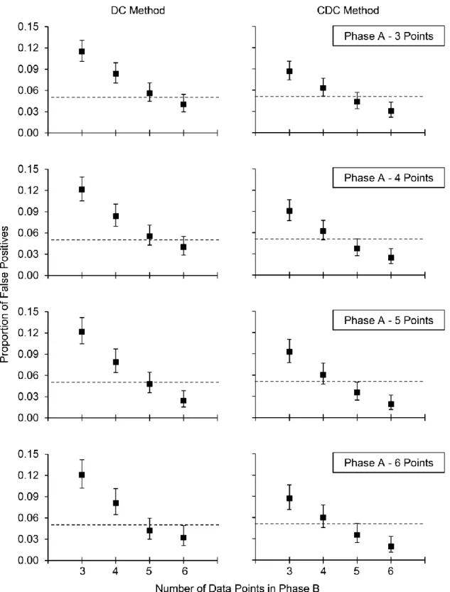
Figure 1 shows the proportion of false positives observed for various phase lengths using the DC and CDC methods. For both methods of analysis, the proportion of false positives decreased systematically when the number of points in Phase B increased. By contrast,
increasing the number of data points in Phase A did not systematically reduce the proportion of false positives when the number of points in Phase B was held constant. For the DC method, the proportion of false positives systematically remained below .05 only when Phase B contained six data points. When Phase B contained five points, type I errors were either marginally above or below the .05 value. By contrast, the CDC method produced false positives for less than 5% of datasets as soon as Phase B contained five data points or more.
From a conceptual standpoint, our results allow us to estimate the probability of observing changes in the absence of the introduction of an independent variable (type I error
rate). Our results indicate that the probability of observing false positives is low when practitioners or researchers collect at least three data points for Phase A and at least five data points for Phase B. In these cases, the alpha level remains near (for the DC method) or below (for the CDC method) .05, which is generally considered acceptable in the research literature.
In general, our results are consistent with prior studies examining false positives in single-case experiments (Fisher et al., 2003; Krueger, Rapp, Ott, Lood, & Novotny, 2013; Novotny et al., 2014). That is, the use of single-case designs did not produce high levels of false positives. Our study further extends the literature by examining the impact of phase length using nonsimulated data. Interestingly, increasing the length of Phase A had marginal effects on the proportion of false positives when compared to Phase B. This observation may be an artifact of the DC and CDC methods, which rely on the number of points in Phase B to determine whether a change was produced or not. When using the DC and CDC methods to supplement visual inspection, our results suggest that researchers and practitioners should conduct at least three baseline and five treatment sessions prior to reversing phases (in ABAB designs) or introducing a new tier (in multiple baseline designs).
Our study has some limitations that should be noted. First, we did not conduct a power analysis as it was not possible with non-simulated data. Researchers and practitioners should weigh power carefully in their choice of an analysis method. Even though the DC method produces slightly more false positives than the CDC method, it is more powerful and thus produces fewer false negatives (Fisher et al., 2003). Second, we used convenience sampling to identify graphs and produced multiple datasets using the same graphs. In the future, researchers should consider randomly selecting graphs and datasets. Finally, we extracted data from only published studies; the characteristics of baseline data from published studies may differ from
those obtained in practical settings (Sham & Smith, 2014). For example, the data paths may be more stable or favorable in published datasets, which could have decreased the likelihood of false positive outcomes. Thus, future studies should consider incorporating datasets from actual practical settings in their analyses.
References
Baer, D. M., Wolf, M. M., & Risley, T. R. (1968). Some current dimensions of applied behavior analysis. Journal of Applied Behavior Analysis, 1, 91-97. doi:10.1901/jaba.1968.1-91 Bourret, J. C., & Pietras, C. J. (2014). Visual analysis in single-case research. In G. J. Madden,
W. V. Dube, T. D. Hackenberg, G. P. Hanley, & K. A. Lattal (Eds.) APA handbook of behavior analysis (pp. 191-218). Washington, DC: American Psychological Association. Fahmie, T. A., & Hanley, G. P. (2008). Progressing toward data intimacy: A review of
within-session data analysis. Journal of Applied Behavior Analysis, 41, 319-331. doi: 10.1901/jaba.2008.41-319
Fisher, W. W., Kelley, M. E., & Lomas, J. E. (2003). Visual aids and structured criteria for improving visual inspection and interpretation of single-case designs. Journal of Applied Behavior Analysis, 36, 387-406. doi:10.1901/jaba.2003.36-387
Huwaldt, J. A. (2015). Plot Digitizer [computer software]. Retrieved from http://plotdigitizer.sourceforge.net/
Krueger, T. K., Rapp, J. T., Ott, L. M., Lood, E. A., & Novotny, M. A. (2013). Detecting false positives in A-B designs: Potential implications for practitioners. Behavior Modification, 37, 615-630. doi:10.1177/0145445512468754
Ninci, J., Vannest, K. J., Willson, V., & Zhang, N. (2015). Interrater agreement between visual analysts of single-case data: A meta-analysis. Behavior Modification, 39, 510-541. doi:10.1177/0145445515581327.
Novotny, M. A., Sharp, K. J., Rapp, J. T., Jelinski, J. D., Lood, E. A., Steffes, A. K., & Ma, M. (2014). False positives with visual analysis for nonconcurrent multiple baseline designs
and ABAB designs: Preliminary findings. Research in Autism Spectrum Disorders, 8, 933-943. doi:10.1016/j.rasd.2014.04.009
Shadish, W. R., & Sullivan, K. J. (2011). Characteristics of single-case designs used to assess intervention effects in 2008. Behavior Research Methods, 43, 971-980.
doi:10.3758/s13428-011-0111-y
Sham, E., & Smith, T. (2014). Publication bias in studies of an applied behavior‐analytic intervention: An initial analysis. Journal of Applied Behavior Analysis, 47, 663-678. doi:10.1002/jaba.146
Smith, J. D. (2012). Single-case experimental designs: A systematic review of published research and current standards. Psychological Methods, 17, 510-550. doi:10.1037/a0029312
Figure 1. Proportion of false positives for different phase lengths when using the dual-criteria (DC; left panels) and conservative dual-criteria (CDC; right panels) methods. The error bars depict the 95% confidence interval for each data point. The dotted line identifies a level of .05.