Modeling of Thermal Mass Energy Storage in Buildings with Phase Change Materials

(1)

UNIVERSITÉ DE MONTRÉAL

MODELING OF THERMAL MASS ENERGY STORAGE IN BUILDINGS WITH PHASE CHANGE MATERIALS

BENOIT DELCROIX

DÉPARTEMENT DE GÉNIE MÉCANIQUE ÉCOLE POLYTECHNIQUE DE MONTRÉAL

THÈSE PRÉSENTÉE EN VUE DE L’OBTENTION DU DIPLÔME DE PHILOSOPHIAE DOCTOR

(GÉNIE MÉCANIQUE) AOÛT 2015

(2)

UNIVERSITÉ DE MONTRÉAL

ÉCOLE POLYTECHNIQUE DE MONTRÉAL

Cette thèse intitulée :

MODELING OF THERMAL MASS ENERGY STORAGE IN BUILDINGS WITH PHASE CHANGE MATERIALS

présentée par : DELCROIX Benoit

en vue de l’obtention du diplôme de : Philosophiae Doctor a été dûment acceptée par le jury d’examen constitué de : M. TRÉPANIER Jean-Yves, Ph. D., président

M. KUMMERT Michaël, Doctorat, membre et directeur de recherche M. DAOUD Ahmed, Ph. D., membre et codirecteur de recherche M. SAVADOGO Oumarou, D. d’état, membre

(3)

DEDICATION

(4)

ACKNOWLEDGEMENTS

This Ph. D. thesis represents a complex work which would have been difficult to realize without the help and the support of people I have met during these four years of Ph. D. studies.

First, I am very grateful to my research director, Professor Michaël Kummert, for his support and trust that he has placed in me during my Ph. D. studies. His friendly guidance, constant questioning and experience have been priceless to me. I will always remember his precious advices during my whole career.

I would like to thank Ahmed Daoud, my co-director and supervisor at Laboratoire des Technologies de l’Énergie (LTE), who have taken over my supervision in the lab and have brought to me his experience and constructive advices. Likewise, I want to thank Jonathan Bouchard, who have been to me an extra co-supervisor in the lab.

I would like to thank all the research group BEE (Bâtiment et Efficacité Énergétique) from the department of Mechanical Engineering, with who I have had wonderful moments at École Polytechnique de Montréal : Aurélie Verstraete, Katherine D’Avignon, Narges Roofigari, Behzad

Barzegar, Corentin Lecomte, Humberto Quintana, Kun Zhang, Massimo Cimmino, Mathieu Lévesque, Romain Jost, Samuel Letellier-Duchesne, Simon Maltais Larouche, and Professor Michel Bernier. I wish to thank in particular Katherine, with who I have “struggled” during long

hours about thorny questions related to phase change materials.

I also thank Professor Philippe Pasquier to have let us carry out thermal conductivity tests using their lab equipment.

I am grateful to all the LTE staff, who has warmly welcomed me during three years. In particular, I would like to thank Michel Dostie, Jocelyn Millette and Éric Dumont, who have made it possible. I also really enjoyed our serious and less serious discussions with Brice Le Lostec, Hervé

Nouanegue and the numerous interns present in the lab.

I wish to thank Marion Hiller, of Transsolar in Stuttgart, for providing us the needed computer tools and for her related help.

I would like to thank professors Jean-Yves Trépanier, Oumarou Savadogo and Dominic Groulx for having accepted being part of my thesis committee.

(5)

The project have been financially supported by Fonds de Recherche du Québec en Nature et Technologies (FRQNT), Natural Sciences and Engineering Research Council of Canada (NSERC) and Hydro-Québec.

Last but not least, I would like to deeply thank my friends and family who support me continuously, just by being themselves.

Thanks to everyone, Benoit Delcroix

(6)

RÉSUMÉ

La masse thermique d’un bâtiment est un paramètre-clé qui détermine la capacité d’un bâtiment à atténuer les variations de température en son sein et d’assurer ainsi un meilleur confort thermique aux occupants. Afin d’augmenter l’inertie thermique de bâtiments à structure légère, des matériaux à changement de phase (MCP) peuvent être utilisés. Ces matériaux offrent en effet une haute capacité de stockage d’énergie (notamment sous forme latente) et un changement de phase à température quasiment constante. Ils s’intègrent aussi parfaitement dans des projets de bâtiments à consommation énergétique nette nulle. L’intérêt actuel pour ceux-ci et pour de meilleures stratégies de gestion de l’appel de puissance requiert des outils capables de simuler des bâtiments hautement isolés possédant une masse thermique importante avec des pas de temps courts (inférieur ou égal à 5 minutes). Ceci représente un défi majeur pour les programmes actuels de simulation énergétique des bâtiments qui ont été développé initialement pour réaliser des calculs horaires. Le modèle de bâtiment utilisé dans le programme TRNSYS présente notamment certains problèmes dans ces circonstances. L’origine de ces problèmes provient de la méthode utilisée pour modéliser la conduction thermique dans les murs. Il s’agit de la méthode des fonctions de transfert. Pour un mur hautement isolé et lourd, la méthode est incapable de générer, pour un pas de temps court, les coefficients supposés représenter la réponse thermique du mur en question. De plus, cette méthode ne permet pas de définir des couches avec des propriétés thermophysiques variables, tels qu’affichés par des MCP. La modélisation de ces MCP est en outre limitée par les informations rendues disponibles par les manufacturiers, qui sont souvent incomplètes ou erronées. Finalement, les modèles actuels simulant des MCP dans les murs ne permettent pas de représenter toute leur complexité. Ceux-ci différencient rarement les processus de fusion et de solidification (hystérèse), prennent en compte occasionnellement la conductivité thermique variable et ne modélisent jamais le sous-refroidissement. Toutes ces problématiques sont soulevées dans cette thèse et des solutions sont proposées.

La première partie (chapitre 4) traite de l’amélioration de la méthode des fonctions de transfert dans TRNSYS grâce à l’utilisation d’un modèle d’état qui permet de diminuer significativement les pas de temps utilisés. La résolution entière de cette problématique est ensuite atteinte en couplant dans TRNSYS un modèle de mur utilisant la méthode aux différences finies à la méthode des fonctions de transfert (chapitre 5).

(7)

La deuxième partie (chapitre 6) s’attelle à caractériser les propriétés thermophysiques d’un MCP utilisé dans divers bancs d’essais, i.e. la densité (annexe A), la conductivité thermique (annexe B) et la capacité thermique. La variété des configurations (MCP en échantillons ou encapsulés dans un film plastique placé dans un mur) et des taux de transfert de chaleur (0.01 à 0.8 °C/min) permet de plus de mettre en évidence l’influence des conditions expérimentales sur le comportement du MCP. La caractérisation est complétée dans le chapitre 7 par une étude du comportement du MCP lors d’interruption de changement de phase (fusion et solidification).

La dernière partie (chapitres 8 et 9) se concentre sur le développement et la validation d’un nouveau modèle permettant de simuler un mur intégrant un ou des MCP (ou plus généralement des couches aux propriétés variables). Le modèle est basé sur une méthode explicite aux différences finies couplée avec une méthode enthalpique pour représenter le comportement du/des MCP. Ce modèle est apte à simuler un MCP avec, à la fois, une hystérèse, un sous-refroidissement et une conductivité thermique variable. Une description détaillée de la méthode et de l’algorithme est donnée. Le modèle est d’abord validé numériquement par comparaison avec des modèles de référence sur 9 cas de murs différents proposés par l’Agence Internationale de l’Énergie. Cette méthode est ensuite comparée à un modèle à capacité thermique effective. Sur 2 aspects (détection du changement de phase et respect de la conservation de l’énergie), la méthode enthalpique développée s’est montrée plus performante que l’autre méthode. Le modèle développé est finalement validé expérimentalement avec des données provenant d’un banc d’essai à échelle réelle.

(8)

ABSTRACT

Building thermal mass is a key parameter defining the ability of a building to mitigate inside temperature variations and to maintain a better thermal comfort. Increasing the thermal mass of a lightweight building can be achieved by using Phase Change Materials (PCMs). These materials offer a high energy storage capacity (using latent energy) and a nearly constant temperature phase change. They can be integrated conveniently in net-zero energy buildings. The current interest for these buildings and for better power demand management strategies requires accurate transient simulation of heavy and highly insulated slabs or walls with short time-steps (lower than or equal to 5 minutes). This represents a challenge for codes that were mainly developed for yearly energy load calculations with a time-step of 1 hour. It is the case of the TRNSYS building model (called Type 56) which presents limitations when modeling heavy and highly insulated slabs with short time-steps. These limitations come from the method used by TRNSYS for modeling conduction heat transfer through walls which is known as the Conduction Transfer Function (CTF) method. In particular, problems have been identified in the generation of CTF coefficients used to model the walls thermal response. This method is also unable to define layers with variable thermophysical properties, as displayed by PCMs. PCM modeling is further hindered by the limited information provided by manufacturers: physical properties are often incomplete or incorrect. Finally, current models are unable to represent the whole complexity of PCM thermal behavior: they rarely include different properties for melting and solidification (hysteresis); they sometimes take into account variable thermal conductivity; but they never model subcooling effects. All these challenges are tackled in this thesis and solutions are proposed.

The first part (chapter 4) focuses on improving the CTF method in TRNSYS through state-space modeling, significantly decreasing the achievable time-steps. A complete solution to this issue can be reached by implementing in TRNSYS a wall model using a finite-difference method and coupling it with the CTF method in Type 56 (chapter 5).

The second part (chapter 6) proposes an in-depth characterization of thermophysical properties of a PCM used in different test-benches, i.e. the density (Appendix A), the thermal conductivity (Appendix B) and the thermal capacity. This section also highlights the influence of the experimental conditions on the PCM thermal behavior: the impact of different configurations (PCM samples or plastic films with encapsulated PCMs located in walls) and different heat transfer

(9)

rates (0.01 to 0.8 °C/min) is discussed. The PCM characterization is completed with a study dedicated to define the PCM thermal behavior when phase change (melting or solidification) is interrupted (chapter 7).

The last part (chapters 8 and 9) focuses on the development and validation of a new model for walls with PCMs, or more generally layers with variable thermal properties. The developed model is based on an explicit finite-difference method coupled with an enthalpy method to model the PCM thermal behavior. This model is able to simulate a PCM with hysteresis, subcooling and temperature-dependent thermal conductivity. A detailed description of the method and the algorithm is given. This model is numerically validated, using comparisons with reference models simulating wall test cases proposed by the International Energy Agency. The developed model is also compared to a reference effective heat capacity model. On two specific aspects (phase change detection and energy conservation principle), the developed enthalpy method is more effective than the other method. Finally, the developed model is experimentally validated using data from a full-scale test-bench.

(10)

LIST OF TABLES

Table 2-1: Most recent and documented PCM models for building walls in TRNSYS ... 31

Table 4-1: Values of the CTF coefficients... 43

Table 4-2: Description of the presented walls ... 45

Table 4-3: Comparison of the minimum timebase value and the calculation time between the DRF and SS methods ... 49

Table 4-4: Description of the external wall in the kitchen (Peeters & Mols, 2012) ... 50

Table 5-1: Evolution of the sum of a set of CTF coefficients and the Fourier number as a function of the timebase for the plain wooden wall ... 56

Table 5-2: Composition of the roof of the studied case (from outside to inside) ... 58

Table 6-1: Summary of the experimental data ... 65

Table 6-2: PCM properties... 67

Table 6-3: Properties of the model for the PCM-equipped wall ... 80

Table 6-4: Thermal capacity definition of the equivalent layer ... 80

Table 7-2: Layers properties ... 95

Table 8-1: TRNSYS PCM models for building walls and their possibilities ... 106

Table 8-2: Material properties ... 112

Table 8-3: Case studies ... 113

Table 8-4: Root mean square deviations [°C] for each case ... 115

Table 8-5: Steady-state surface heat-flows [W/m²] (after 120 hours) ... 116

Table 8-6: Normalized 𝑅𝑀𝑆𝐷 for each case [%]... 117

Table 8-7: CPU time depending on the number of nodes and the internal time-step for a 120-hour simulation ... 118

(16)

Table 8-9: Surface heat-flows differences for cases 3 and 8 ... 119

Table 8-10: PCM properties for the phase change detection issue case ... 120

Table 8-11: Layers properties for the subcooling issue case (from outside to inside) ... 125

Table 9-2: U-values, infiltration and dimensions of test-cells ... 140

Table 9-3: Tested scenarios in 2013 ... 141

Table 9-4: Layers properties of the PCM-equipped wall ... 148

Table 9-5: RMSD values between experiments and simulations for the scenarios illustrated in Figure 9-16 and Figure 9-17 ... 152

Table 9-6: Computation times for the test-cell simulations with the extreme set-back scenario (146-hour simulation with a 1-min time-step) ... 152

Table 9-7: Connections between Type 56 and the external wall type ... 155

Table A-1: Density measurements of 10 PCM samples ... 178

Table C-1: Thickness and thermal conductivity of each material in the PCM-equipped wall .... 182

Table D-1: List of parameters ... 186

Table D-2: List of inputs ... 191

(17)

LIST OF FIGURES

Figure 1-1: Prediction of the average hourly power demand in the province of Québec in January

and July 2007 (Hydro-Québec, 2006) ... 1

Figure 2-1: Heat balance method (ASHRAE, 2013) ... 6

Figure 2-2: CTF method ... 10

Figure 2-3: 1-D two-node model of a wall ... 13

Figure 2-4: 1-D finite-difference grid ... 15

Figure 2-5: Explicit scheme ... 17

Figure 2-6: Implicit scheme ... 18

Figure 2-7: Crank-Nicolson scheme ... 19

Figure 2-8: Two different approaches of T-history tests ... 22

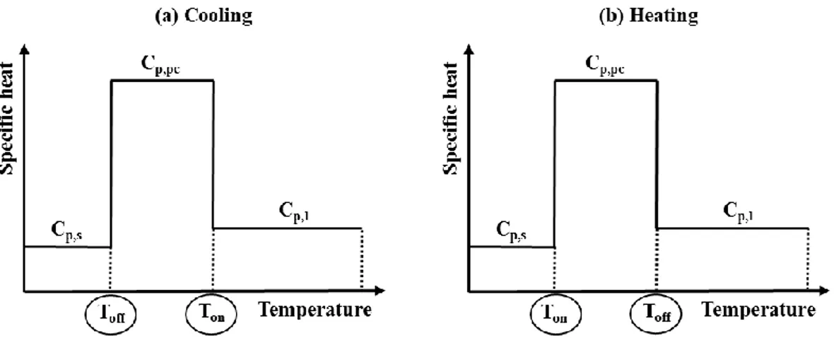
Figure 2-9: (a) Specific-heat – temperature and (b) enthalpy – temperature curves of a PCM with a phase change temperature range [𝑇𝑠,𝑇𝑙] ... 24

Figure 2-10: PCM hysteresis... 28

Figure 2-11: PCM subcooling ... 29

Figure 2-12: Possible behavior of a PCM cooled down after partial melting ... 29

Figure 4-1: Scheme of a three-node example ... 41

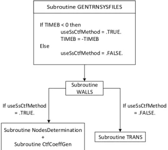
Figure 4-2: Scheme of the implementation of the SS method in TRNSYS ... 44

Figure 4-3: Description of the presented scenario ... 46

Figure 4-4: Evolution of the inside surface temperature for an ICF wall ... 47

Figure 4-5: Evolution of the inside surface temperature for an ICF wall (zoom)... 47

Figure 4-6: Evolution of the inside surface temperature for a wooden wall ... 48

Figure 4-7: Evolution of the inside surface temperature for a wooden wall (zoom) ... 48

Figure 4-8: Picture of the house in project ZEHR (Zero Energy House Renovation) (Peeters & Mols, 2012) ... 50

(18)

Figure 4-9: Plan of the house’s ground floor (Peeters & Mols, 2012) ... 50

Figure 4-10: Evolution of the operative temperature in the kitchen [corrected after publication] 51 Figure 5-1: Error window when TRNBuild fails to generate transfer function coefficients ... 56

Figure 5-2: Complementarity of the CTF method and the finite-difference methods ... 58

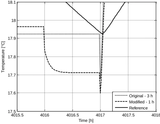
Figure 5-3: Test case with temperature step-changes... 59

Figure 5-4: Results comparison between both configurations ... 59

Figure 6-1: Schematic representation of the hysteresis and subcooling effects ... 63

Figure 6-2: Plastic film with PCM pouches ... 66

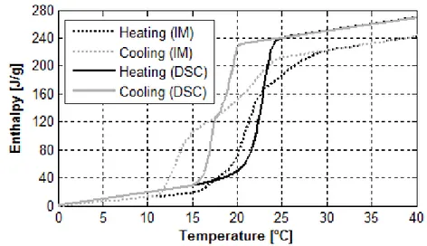
Figure 6-3: (a) Differential Scanning Calorimetry test (2 °C/min) and (b) resulting enthalpy-temperature curves (adapted from (Phase change energy solutions, 2008)) ... 68

Figure 6-4: Principle of the T-history experimentation ... 69

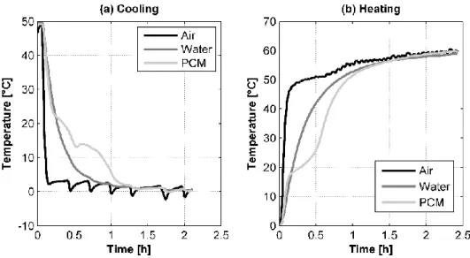
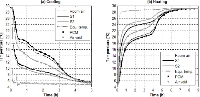
Figure 6-5: Temperature evolutions of the air, water and PCM during (a) cooling and (b) heating processes ... 69

Figure 6-6: R-C model for the water sample ... 71

Figure 6-7: R-C model for the PCM sample (top-view) ... 71

Figure 6-8: Comparison between simulated and measured data for the water sample during (a) cooling and (b) heating processes ... 73

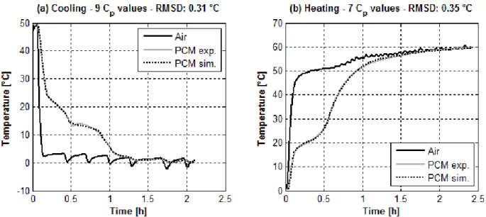
Figure 6-9: Comparison between experimental and simulated temperature evolution of the PCM sample during (a) cooling and (b) heating processes ... 74

Figure 6-10: Comparison between the enthalpy-temperature curves of the inverse method (IM) and the DSC test ... 75

Figure 6-11: Schematic of the instrumented PCM-equipped walls ... 76

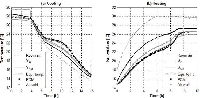
Figure 6-12: Experimental data for a cooling-heating cycle in the dual temperature chamber ... 77

Figure 6-13: Picture and top-view of the test cell with PCM-equipped walls ... 78

(19)

Figure 6-15: Experimental data for a cooling-heating cycle in the test-cell ... 79

Figure 6-16: Modeling of the PCM-equipped wall ... 80

Figure 6-17: Graphs explaining the variables to be optimized during (a) cooling and (b) heating processes ... 81

Figure 6-18: Comparison between experimental and simulated temperature evolution for wall experimentations during (a) cooling and (b) heating processes ... 81

Figure 6-19: Comparison between experimental and simulated temperature evolution for test-cell experimentations during (a) cooling and (b) heating processes ... 82

Figure 6-20: Variation of the phase change temperature range as a function of the (a) cooling and (b) heating rates ... 83

Figure 6-21: Variation of the hysteresis effect as a function of the cooling / heating rates ... 83

Figure 6-22: Comparison of ℎ(𝑇) curves for both (a) cooling and (b) heating processes ... 84

Figure 7-1: Possible behavior of a PCM cooled down after partial melting ... 92

Figure 7-2: 1-D finite-difference model of a wall ... 93

Figure 7-3: Instrumented PCM-equipped wall ... 95

Figure 7-4: (a) PCM-equipped wall model; (b) Enthalpy-temperature curves of the equivalent layer ... 95

Figure 7-5: Experimental data for the interrupted heating (a) and cooling (b) scenarios ... 96

Figure 7-6: Comparison between experimental and simulated data for the interrupted heating (a) and cooling (b) scenarios ... 97

Figure 7-7: Comparison between experimental and optimized simulated data for the interrupted heating (a) and cooling (b) scenarios ... 97

Figure 7-8: Thermal behavior mapping of the optimized solution ... 98

Figure 8-1: (a) PCM specific effects and (b) transitional PCM thermal behavior during phase change ... 104

(20)

Figure 8-3: Process scheme of the algorithm ... 111

Figure 8-4: Schematic zones of an enthalpy-temperature graph used during simulation ... 112

Figure 8-5: (a) Specific heat-temperature curve and (b) thermal conductivity-temperature curve of the PCM used in the test cases ... 113

Figure 8-6: Initial and boundary conditions used for the test cases ... 114

Figure 8-7: Comparison between reference models and the new model for each case ... 115

Figure 8-8: Results comparison between models with a different number of nodes for 2 cases . 118 Figure 8-9: Phase change detection issue ... 120

Figure 8-10: Initial and boundary conditions used for the phase change detection issue case .... 120

Figure 8-11: Results comparison between TRNSYS Type 399 and Type 3258 for the phase change detection issue case ... 121

Figure 8-12: Illustration of the problem caused by an instantaneous switch between cooling and heating 𝐶𝑝(𝑇) curves ... 123

Figure 8-13: Practical consequence caused by an instantaneous switch between cooling and heating 𝐻(𝑇) curves ... 123

Figure 8-14: Subcooling modeling issue ... 124

Figure 8-15: Enthalpy-temperature curves for the subcooling issue case ... 125

Figure 8-16: Initial and boundary conditions used for the subcooling issue case ... 125

Figure 8-17: PCM temperature results for the subcooling issue case (zoom on subcooling (b)) 126 Figure 8-18: Outside (a) and inside (b) surface temperature results for the subcooling issue case ... 126

Figure 9-1: 1-D finite-difference of a 1-layer wall... 134

Figure 9-2: Principle of the coupling between Type 56 and the external PCM wall model ... 136

Figure 9-3: TRNSYS solution methodology (adapted from (Jost, 2012)) ... 137

(21)

Figure 9-5: (a) DSC test and (b) resulting enthalpy-temperature curves (adapted from (Phase

change energy solutions, 2008)). ... 138

Figure 9-6: Instrumented PCM-equipped wall ... 139

Figure 9-7: Test-bench description... 139

Figure 9-8: (a) Evolution of temperatures inside the test-cells and in the center of the added walls (with and without PCMs) and (b) evolution of the heating power during residential workday scenario (17-03 and 18-03) ... 142

Figure 9-9: (a) Evolution of temperatures inside the test-cells and in the center of the added walls (with and without PCMs) and (b) evolution of the heating power during CI scenario (26-03 and 27-03) ... 143

Figure 9-10: Evolution of the temperature gradient in the added walls without (a) and with (b) PCM during the extreme set-back scenario (13-04 and 14-04) ... 144

Figure 9-11: Illustration of the temperature heterogeneity in the PCM-equipped wall (13-04 and 14-04) ... 145

Figure 9-12: Heating consumption for different scenarios with and without PCM ... 145

Figure 9-13: Comparison between experimental and simulated results for the test-cell without PCM during the extreme set-back scenario (from 11-04-2013 to 17-04-2013) ... 147

Figure 9-14: Enthalpy-temperature curves of the equivalent layer ... 148

Figure 9-15: Comparison between experimental and simulated results for the test-cell with PCM during the extreme set-back scenario (from 11-04-2013 to 17-04-2013) ... 149

Figure 9-16: Results comparison between the test-cells equipped with and without PCMs during the residential workday scenario (from 11-03-2013 to 15-03-2013)... 150

Figure 9-17: Results comparison between the test-cells equipped with and without PCMs during the commercial and institutional scenario (from 25-03-2013 to 28-03-2013) ... 151

Figure 9-18: Proposed methodology to link an external wall type to Type 56... 155

Figure A-1: Density test proceedings ... 177

(22)

Figure B-1: Hot-wire equipment scheme ... 180 Figure B-2: Comparison between the manufacturer values and the experimental values of thermal conductivity in liquid (L) and solid (S) states ... 181 Figure C-1: Scheme of the PCM-equipped wall ... 182

(23)

LIST OF SYMBOLS AND ABBREVIATIONS

𝐴 Area [m²]

𝑎, 𝑏, 𝑐, 𝑑 Conduction transfer function coefficients

Bi Biot number [-] 𝐶 Capacitance [J/m²-K] 𝐶_𝑝 Specific heat [J/g-K] Fo Fourier number [-] 𝐻 Enthalpy [J/kg] ℎ Coefficient of convection [W/m²-K] ℎ_𝑔 Global heat transfer coefficient [W/m²-K] 𝑘 Thermal conductivity [W/m-K]

𝐿 Latent heat [J/kg]

𝐿_𝑐 Characteristic length [m] 𝑙_𝑓 Liquid fraction [-]

𝑛_𝑎, 𝑛_𝑏, 𝑛_𝑐, 𝑛_𝑑 Number of coefficients 𝑎, 𝑏, 𝑐 and 𝑑

𝒪 Truncation error 𝑄 Energy [J] 𝑞̇ Heat flow [W] 𝑅 Thermal resistance [m²-K/W] St Stefan number [-] 𝑠 Laplace variable 𝑇 Temperature [°C] 𝑡 Time [s]

(24)

𝑥 Position [m] ∆𝑡 Time-step [s] ∆𝑡_𝑏 Timebase (CTF time-step) [s] Greek symbols 𝛼 Thermal diffusivity [m²/s] 𝜌 Density [kg/m³] 𝜏 Time constant [s] Subscripts 𝑎𝑏𝑠 Absorbed

𝐶𝐿 Convective parts of internal loads 𝑐𝑜𝑛𝑑 Conductive

𝑐𝑜𝑛𝑣 Convective

𝑒𝑞 Equipment

𝑖 Inside

𝐼𝑉 Infiltration and/or ventilation 𝑗 Iteration level 𝑙 Liquid 𝐿𝑊𝑅 Long-wave radiation 𝑛 Node 𝑜 Outside 𝑝𝑐 Phase change 𝑟𝑎𝑑 Radiative 𝑠 Surface or solid 𝑠𝑜𝑙 Solar

(25)

𝑆𝑊 Short-wave radiation

𝑠𝑦𝑠 System

Abbreviations

1-D One-dimensional

3-D Three-dimensional

BPS Building performance simulation BTCS Backward time and central space

C-N Crank-Nicolson

CTF Conduction transfer function DLL Dynamic-link library

DRF Direct-root finding

DSC Differential scanning calorimetry FD Finite-difference

FTCS Forward time and central space LTI Linear time-invariant

PCM(s) Phase change material(s) RMSD Root mean square deviation

(26)

LIST OF APPENDICES

Appendix A – Experiments on PCM density ... 177 Appendix B – Experiments on PCM thermal conductivity ... 180 Appendix C – Equivalent layer thermal conductivity ... 182 Appendix D – Proforma of TRNSYS Type 3258 ... 184

(27)

CHAPTER 1 INTRODUCTION

Building thermal mass is a key parameter to mitigate inside temperature variations. Used with an optimized control strategy, a thermal mass increase is a solution to maintain a better thermal comfort, to stabilize heating and cooling loads and to mitigate peak power demand. In Québec, more than two thirds of households live in all-electric houses and are therefore partially responsible for the electric grid peaks, especially during winter (Leduc, Daoud, & Le Bel, 2011). The share of all-electric houses is expected to rise even higher in the future, mainly because of the fluctuations in oil and gas prices compared to the stable – and low – electricity prices in the province. Québec is almost entirely (more than 90 %) supplied by hydroelectric installations (Ministère des Ressources naturelles et de la Faune, 2010). In winter, the maximum power peak demand can reach up to approximately 40 GW (Leduc et al., 2011), which represents 103 % of the capacity managed by Hydro-Québec, 90 % of the capacity installed in Québec, or 80 % of the capacity available in Québec (including Churchill falls installations in the province of Newfoundland) (Ministère des Ressources naturelles et de la Faune, 2010). An increasing number of all-electric buildings will require additional power capacity in order to guarantee the future electric supply, unless effective peak load management strategies are implemented.

Figure 1-1 presents the prediction of the average power demand in Québec in January and July 2007 performed by Hydro-Québec in 2006. Clear seasonal and hourly differences are observed.

Figure 1-1: Prediction of the average hourly power demand in the province of Québec in January and July 2007 (Hydro-Québec, 2006)

(28)

A higher power demand is observed during winter, caused mainly by buildings heating loads. Two peaks are distinguished during winter in the morning and the evening, corresponding to the beginning and the end of regular working days. During summer, the power demand is mainly driven by the daily schedule of most human activities, and the impact of building cooling loads is comparatively lower than the impact of heating loads.

Strong variations of the peak power demand are a source of instability for the electrical network in Québec. Increasing buildings thermal mass can contribute to mitigate these variations by spreading out the energy consumption over time. An interesting option to achieve this goal is the addition of phase change materials (PCMs) to building walls, floors and ceilings. Their latent energy storage capacity coupled with their nearly isothermal phase change temperature are significant assets. Compared to heavy materials such as concrete, PCMs have the advantage of storing more energy in more compact and lighter materials. Currently, PCMs are mainly used for cooling applications in countries with warmer climates. But PCMs also have a potential in colder climates for heating applications.

However using PCMs in the building envelope remains marginal and only few commercial products are available. Companies such as Phase Change Energy Solutions (2014) and DuPont (2012) have developed and commercialized products which can be easily implemented directly in building walls.

As with any other energy conservation or peak power reduction measure, the impact of adding PCMs to the building envelope must be assessed through a detailed analysis involving Building Performance Simulation (BPS) programs such as TRNSYS, EnergyPlus or ESP-r. Assessing peak power demand management strategies requires accurate transient simulations of highly insulated and heavy walls with short time-steps (< 5 minutes). This represents a challenge for most BPS tools, which are primarily dedicated to yearly energy performance analysis with an hourly time-step. This is for example the case in TRNSYS, where the building model (known as Type 56) presents some limitations in this particular context. These limitations come from the method used to model 1-D thermal conduction through walls, which is known as the Conduction Transfer Function (CTF) method. Moreover, the CTF method is not designed to simulate building materials with temperature-dependent properties, such as experienced by PCMs. A finite-difference method is then preferably used in order to overcome these limitations. The PCM temperature-dependent

(29)

thermal capacity is generally modeled with enthalpy-temperature or specific-heat-temperature curves. Unfortunately, most models do not include the whole complexity of PCMs thermal behavior. A differentiation between heating and cooling processes is rarely modeled while subcooling is almost never taken into account.

Modeling a PCM requires to know its thermophysical properties, i.e. density, thermal conductivity and capacity. Manufacturers document most of the time these main properties. However, these data are generally incomplete or not representative. For example, the definition of the thermal conductivity is often given with only one value, while PCM thermal conductivity is actually variable, depending on its temperature and state (liquid or solid). Likewise, the PCM thermal capacity values provided by manufacturers are often incomplete and do not always represent the actual final product. Few data sheets provided by manufacturers include enthalpy-temperature or specific heat-temperature curves for heating and cooling processes. If provided, these curves are most often obtained using Differential Scanning Calorimetry (DSC) tests. This method uses small samples (a few milligrams) and imposes high heat fluxes to the sample, which is not representative of PCMs implemented in building walls (large quantity of PCMs, relatively low heat fluxes and temperature variations).

The three main objectives of this thesis result from the above-mentioned issues and two of them are composed of several more specific goals:

- Improvement of the CTF method in TRNSYS to allow accurate low-time-step simulations of buildings with highly resistive and heavy walls.

- Accurate and representative characterization of a selected PCM:

o Evaluation of the density and thermal conductivity through experimentations.

o Evaluation of the temperature-dependent thermal capacity based on inverse methodology and analysis of the impacts of different configurations (PCM samples of a few grams or walls equipped with PCMs) and varying heating / cooling rates on this property.

o In the case of a PCM with 2 enthalpy-temperature curves (heating and cooling): identification of the PCM thermal behavior when phase change is interrupted.

- Accurate modeling of a wall with PCMs, considering all aspects of the PCM thermal behavior complexity:

(30)

o Development of a model of wall including PCM(s) or layer(s) with temperature-dependent properties.

o Numerical validation of the developed model through a comparison with reference models for several wall test cases.

o Experimental validation of the developed model using experimental data from a full-scale test-bench.

Preliminary notes and clarifications:

a) In the present thesis, it is indicated that DSC tests should not be used to determine the 𝐻(𝑇) curves because they are not representative of the way how PCMs are used in the building envelope. DSC tests are intended to obtain the latent heat and the melting temperature of a PCM, but they are often used by practitioners and researchers in building sciences to obtain the 𝐻(𝑇) curve of a PCM. The work in this thesis shows that the 𝐻(𝑇) curves obtained through this method are not applicable to the PCM encapsulation techniques and thermal solicitations typically found in buildings. Rather than the DSC tests, it is the extrapolated 𝐻(𝑇) curves that cannot be used.

b) In this thesis, the term “subcooling” is used to denote the phenomenon observed when a PCM is cooled below its solidification temperature, which is followed by a sudden temperature increase (after a perturbation) leading to solidification. This phenomenon is more properly denoted by supercooling.

c) The experimental results presented in this thesis aim to show that phase change differs depending on the experimental conditions, especially the phase change temperature range during melting and solidification. In this thesis, phase change temperature range denotes the temperature “plateau” observed in graphs showing PCM temperature evolutions and defined between two temperatures, often interpreted as the “onset” and “offset” of fusion or solidification. Below the lower temperature, the PCM is assumed solid. On the other hand, the PCM is supposed liquid if the measured temperature is beyond the upper temperature. These interpretations are often found in the scientific literature but may not be strictly accurate from the chemical point of view.

(31)

d) Temperature measurements during all experimentations presented in this thesis are performed using T-type thermocouples, having a measurement uncertainty of ± 0.5 °C.

(32)

CHAPTER 2 LITERATURE REVIEW

This literature review first discusses heat transfer modeling in Building Performance Simulation (BPS) tools (section 2.1), focusing on transient conduction through walls (section 2.2). The modeling of transient conduction heat transfer with the presence of PCMs is then presented in section 2.3.

2.1 Heat transfer modeling in buildings

Most BPS programs such as TRNSYS (Klein et al., 2012), EnergyPlus (Crawley et al., 2001) and ESP-r (Energy Systems Research Unit, 1998) are based on the heat balance methodology for modeling the whole heat transfer in buildings. This method is illustrated in Figure 2-1 (ASHRAE, 2013).

Figure 2-1: Heat balance method (ASHRAE, 2013)

The heat balance method can be viewed as four distinct processes (as suggested in Figure 2-1): a) Outdoor face heat balance

(33)

For each surface, the heat balance on the outdoor face depends on the absorbed solar radiation

𝑞̇_{𝑎𝑏𝑠,𝑠𝑜𝑙}, the net long-wave radiation exchange 𝑞̇_𝐿𝑊𝑅 with the sky and the surroundings, the

convective exchange 𝑞̇_{𝑐𝑜𝑛𝑣} with the outside air and the conductive heat transfer into the wall

𝑞̇_{𝑐𝑜𝑛𝑑,𝑜}. It can be formulated as follows:

𝑞̇_{𝑎𝑏𝑠,𝑠𝑜𝑙}+ 𝑞̇_𝐿𝑊𝑅 + 𝑞̇_{𝑐𝑜𝑛𝑣,𝑜}− 𝑞̇_{𝑐𝑜𝑛𝑑,𝑜} = 0 ( 2.1 )

The first three terms of Equation ( 2.1 ) are positive for net heat flows to the outdoor face. The conductive term is considered positive from outdoors to inside the wall.

b) Heat conduction through walls

Many methods have been developed for modeling heat conduction through walls. They are based on time series methods, transform methods or numerical methods. This problem, which is at the core of this thesis, is discussed further in section 2.2 for methods used to model heat conduction through walls with constant properties and in section 2.3 for walls including PCMs or layer(s) with variable properties.

c) Indoor face heat balance

As for the outdoor face, the heat balance on the indoor face involves all heat transfer modes (conduction, convection and radiation) and is composed of:

- The net long-wave radiative exchange between zone surfaces 𝑞̇_{𝐿𝑊𝑅,𝑠}. - The long-wave radiation from equipment 𝑞̇_{𝐿𝑊𝑅,𝑒𝑞}.

- The short-wave radiation from lights to surface 𝑞̇_𝑆𝑊.

- The conductive heat transfer through wall (outside to inside) 𝑞̇_{𝑐𝑜𝑛𝑑,𝑖}. - The transmitted solar radiation absorbed at surface 𝑞̇_𝑠𝑜𝑙.

- The convective heat transfer to zone air 𝑞̇_{𝑐𝑜𝑛𝑣,𝑖}. The indoor face heat balance is therefore formulated such as:

𝑞̇_{𝐿𝑊𝑅,𝑠}+ 𝑞̇_{𝐿𝑊𝑅,𝑒𝑞}+ 𝑞̇_𝑆𝑊 + 𝑞̇_{𝑐𝑜𝑛𝑑,𝑖}+ 𝑞̇_𝑠𝑜𝑙 − 𝑞̇_{𝑐𝑜𝑛𝑣,𝑖}= 0 ( 2.2 )

(34)

The last balance to be performed is on the zone air. It is formulated as follows:

𝑞̇_𝐼𝑉+ 𝑞̇_𝐶𝐸+ 𝑞̇_𝑠𝑦𝑠+ 𝑞̇_{𝑐𝑜𝑛𝑣,𝑖} = 0 ( 2.3 )

Where:

- 𝑞̇_𝐼𝑉 is the sensible load caused by infiltration and ventilation.

- 𝑞̇𝐶𝐸 is the convective gains of internal loads (e.g. heat released by occupants). - 𝑞̇_𝑠𝑦𝑠 is the heat transfer to/from HVAC system.

- 𝑞̇_{𝑐𝑜𝑛𝑣,𝑖} is the convection from all surfaces.

The three first elements a) to c) are duplicated for each surface while the last (air heat balance) is carried out for each air node.

2.2 1-D conduction heat transfer modeling through walls

Transient heat conduction in BPS programs is mainly modeled using two methods. First, the Conduction Transfer Function (CTF) method is an analytical method and is for example used in TRNSYS and EnergyPlus. Secondly, finite-difference methods are numerical methods and are used in ESP-r and optionally in EnergyPlus. Prior to reviewing these methods, a brief reminder on the Fourier law and two important dimensionless numbers is presented.

2.2.1 Fourier law and dimensionless numbers

Conduction heat transfer was experimentally defined by Fourier (1822), who formulated the following relationship:

𝑑𝑄

𝑑𝑡 = −𝑘 𝐴 𝑑𝑇

𝑑𝑥 ( 2.4 )

Equation ( 2.4 ) indicates that the heat flow is proportional to the heat exchange surface 𝐴, the thermal conductivity 𝑘 and the temperature gradient between 2 points.

In order to characterize transient conduction problems, two dimensionless numbers are of interest: Fourier and Biot numbers.

(35)

Named after Fourier, this number Fo is the ratio of the heat conduction rate to the rate of thermal energy storage in a solid (Bergman, Lavine, Incropera, & Dewitt, 2011). It is sometimes defined as dimensionless time. It is formulated as follows:

Fo =𝛼 ∆𝑡 𝐿2𝑐

( 2.5 )

Where 𝐿_𝑐 is the characteristic length and the thermal diffusivity 𝛼 depends on the thermal conductivity 𝑘, on the density 𝜌 and on the specific heat 𝐶𝑝 and is computed such as:

𝛼 = 𝑘

𝜌 𝐶_𝑝 ( 2.6 )

Physically a lower Fourier number means a lower heat transmission rate. It also means that the thermal mass increases.

The second dimensionless number is the Biot number. It is defined as the ratio of the internal thermal resistance of a solid to the boundary layer thermal resistance (Bergman et al., 2011). This number is mathematically expressed as follows:

Bi =ℎ 𝐿𝑐

𝑘 ( 2.7 )

Where ℎ is the convective heat transfer coefficient.

A Biot number with a value higher than 1 means that the heat transmission rate is lower inside the material than at its surface. It also indicates a significant temperature gradient inside the material. This temperature gradient is theoretically assumed negligible if the Biot number is equal to or lower than 0.1. Computing the Biot number is also a way to validate the conformity of using a lumped capacitance model.

2.2.2 Conduction transfer function method

CTF method is used in BPS programs like TRNSYS to model 1-D transient heat conduction through building walls with constant thermophysical properties. This method was primarily developed by Stephenson and Mitalas (1971) and consists in computing the Conduction Transfer Functions by solving the heat conduction equation with the Laplace and Z transforms theory. Later,

(36)

Mitalas and Arseneault (1972) developed an algorithm to compute the CTF coefficients, based upon the method of Stephenson and Mitalas.

Figure 2-2: CTF method

Conduction Transfer Functions solve linear time invariant (LTI) systems from time series composed of current and past inputs and past outputs. In TRNSYS, the CTF method computes the inside and outside surface heat flows 𝑞̇_𝑠𝑖 and 𝑞̇_𝑠𝑜 from current and past values of the inside and outside surface temperatures 𝑇_𝑠𝑖 and 𝑇_𝑠𝑜 and from the past outputs values (𝑞̇_𝑠𝑖 and 𝑞̇_𝑠𝑜) (Figure 2-2): 𝑞̇_{𝑠𝑖,𝑡} = ∑ 𝑏_{𝑡−𝑖∆𝑡}_𝑏 𝑇_{𝑠𝑜,𝑡−𝑖∆𝑡}_𝑏 𝑛𝑏 𝑖=0 − ∑ 𝑐_{𝑡−𝑖∆𝑡}_𝑏 𝑇_{𝑠𝑖,𝑡−𝑖∆𝑡}_𝑏 𝑛𝑐 𝑖=0 − ∑ 𝑑_{𝑡−𝑖∆𝑡}_𝑏 𝑞̇_{𝑠𝑖,𝑡−𝑖∆𝑡}_𝑏 𝑛𝑑 𝑖=1 ( 2.8 ) 𝑞̇_{𝑠𝑜,𝑡} = ∑ 𝑎_{𝑡−𝑖∆𝑡}_𝑏 𝑇_{𝑠𝑜,𝑡−𝑖∆𝑡}_𝑏 𝑛𝑎 𝑖=0 − ∑ 𝑏_{𝑡−𝑖∆𝑡}_𝑏 𝑇_{𝑠𝑖,𝑡−𝑖∆𝑡}_𝑏 𝑛𝑏 𝑖=0 − ∑ 𝑑_{𝑡−𝑖∆𝑡}_𝑏 𝑞̇_{𝑠𝑜,𝑡−𝑖∆𝑡}_𝑏 𝑛𝑑 𝑖=1 ( 2.9 )

Where the coefficients 𝑎, 𝑏, 𝑐 and 𝑑 must meet the following requirement: ∑𝑛𝑎 𝑎_{𝑡−𝑖∆𝑡}_𝑏 𝑖=0 ∑𝑛𝑑 𝑑_{𝑡−𝑖∆𝑡}_𝑏 𝑖=0 = ∑ 𝑏𝑡−𝑖∆𝑡𝑏 𝑛𝑏 𝑖=0 ∑𝑛𝑑 𝑑_{𝑡−𝑖∆𝑡}_𝑏 𝑖=0 = ∑ 𝑐𝑡−𝑖∆𝑡𝑏 𝑛𝑐 𝑖=0 ∑𝑛𝑑 𝑑_{𝑡−𝑖∆𝑡}_𝑏 𝑖=0 = 𝑈 ( 2.10 )

∆𝑡_𝑏 is named the timebase and is the CTF time-step. It must be equal to or an integer multiple of the simulation time-step. If 𝑖 equals 0 in Equations ( 2.8 ) to ( 2.10 ), it means the current time-step. If 𝑖 equals 1, it then means the previous time-step. And so on until it reaches the number of coefficients.

(37)

Equations ( 2.8 ) and ( 2.9 ) depend on the current surface temperatures 𝑇_𝑠𝑖 and 𝑇_𝑠𝑜, which are unknown. Surface temperatures depend on net convective and radiative heat gains with the surroundings but also on the heat conduction through the wall. Surface heat balance is solved using an iterative procedure, as explained and suggested by Mitalas (1968).

Coefficients 𝑎, 𝑏, 𝑐 and 𝑑 characterize the thermal behavior of a wall and can be generated using several methods, which were for example compared by Li et al. (2009). The mainly used two methods are the Direct Root Finding (DRF) and State-Space (SS) methods. The first was developed by Mitalas, Stephenson and Arseneault (Mitalas & Arseneault, 1972; Stephenson & Mitalas, 1971) and is used in TRNSYS. On the other hand, the latter was developed by Ceylan, Myers and Seem (Ceylan & Myers, 1980; Seem, 1987) and is implemented in EnergyPlus.

2.2.2.1 Direct Root Finding method

This method is based on Pipe’s method (1957) for computing heat flows through walls, which is also documented by Carslaw and Jaeger (1959). Pipe shows that the Laplace transforms of the heat flow and temperature at inside and outside wall surfaces are related by the following matrix expression: [𝑇𝑠𝑜(𝑠) 𝑞̇_𝑠𝑜(𝑠)] = [ 𝐴(𝑠) 𝐵(𝑠) 𝐶(𝑠) 𝐷(𝑠)] [ 𝑇_𝑠𝑖(𝑠) 𝑞̇_𝑠𝑖(𝑠)] ( 2.11 )

Where 𝑠 is the Laplace variable, and:

𝐴(𝑠) = 𝐷(𝑠) = cosh (𝐿√𝑠 𝛼) ( 2.12 ) 𝐵(𝑠) = − R sinh (𝐿√_𝛼)𝑠 𝐿 √_𝛼𝑠 ( 2.13 ) 𝐶(𝑠) = − 𝐿√_{𝛼 sinh (𝐿√}𝑠 _𝛼)𝑠 𝑅 ( 2.14 )

(38)

The square matrix in Equation ( 2.11 ) is called transmission matrix and is further shortened conveniently as [𝑀]. For a multilayer wall, the transmission matrix is the product of matrices of each layer. For a n-layer wall, the transmission matrix is therefore:

[𝑀] = [𝑀₁][𝑀₂] … [𝑀_𝑛] ( 2.15 )

If one of the layer is purely resistive (no thermal mass), the transmission matrix is as follows: [1 −𝑅

0 1 ].

The determinant of all transmission matrices is one. Equation ( 2.11 ) can then be rearranged in order to relate the inputs (𝑇_𝑠𝑖 and 𝑇_𝑠𝑜) to the outputs (𝑞̇_𝑠𝑖 and 𝑞̇_𝑠𝑜), as needed in Equations ( 2.8 ) and ( 2.9 ). The following expression is obtained:

[𝑞̇𝑠𝑜(𝑠) 𝑞̇_𝑠𝑖(𝑠)] = [ 𝐷(𝑠) 𝐵(𝑠) − 1 𝐵(𝑠) 1 𝐵(𝑠) − 𝐴(𝑠) 𝐵(𝑠)] [𝑇𝑠𝑜(𝑠) 𝑇_𝑠𝑖(𝑠)] ( 2.16 )

The transmission matrix is composed of four transfer functions which relate each input to each output. Equation ( 2.16 ) is a continuous expression and has to be discretized with a sampling interval equivalent to the timebase ∆𝑡𝑏 using Z-transform theory in order to compute the CTF coefficients. This stage requires computing the roots of 𝐵(𝑠) with a numerical root-finding procedure. For highly resistive and heavy walls, the root-finding procedure can miss several roots and can therefore be unable to generate the CTF coefficients. Hittle and Bishop (1983) discussed this issue and developed an improved root-finding procedure.

Once the roots of 𝐵(𝑠) obtained, the CTF coefficients are computed, as explained by Stephenson and Mitalas (1971) or more recently by Giaconia and Orioli (2000).

2.2.2.2 State-Space method

The State-Space (SS) method is used in EnergyPlus for generating CTF coefficients. It was initially developed by Ceylan and Myers (1980) to model multidimensional heat transfer with transfer functions generated from a set of first order differential equations. Seem (1987) improved this method by generating only significant coefficients and therefore decreasing their numbers.

(39)

Myers (1971) showed that a heat transfer problem can be modeled with a state-space representation, using finite-difference method to spatially discretize the problem. Heat transfer problems can then be presented such as LTI systems with 𝑛_𝑠 states, 𝑛_𝑖 inputs and 𝑛_𝑜 outputs:

𝑑 [ 𝑇1 … 𝑇_𝑛 ] 𝑑𝑡 = [𝐴] [ 𝑇1 … 𝑇_𝑛 ] + [𝐵] [𝑇𝑖 𝑇_𝑜] ( 2.17 ) [𝑞̇𝑖 𝑞̇𝑜] = [𝐶] [ 𝑇1 … 𝑇_𝑛 ] + [𝐷] [𝑇𝑖 𝑇_𝑜] ( 2.18 )

Where 𝐴, 𝐵, 𝐶 and 𝐷 are matrices with constant coefficients. Their sizes are respectively (𝑛_𝑠,𝑛_𝑠), (𝑛_𝑠,𝑛_𝑖), (𝑛_𝑜,𝑛_𝑠) and (𝑛_𝑜,𝑛_𝑖). Temperatures 𝑇_𝑖 and 𝑇_𝑜 are inputs. Heat flows 𝑞̇_𝑖 and 𝑞̇_𝑜 are outputs. The vector including temperatures 𝑇₁ to 𝑇_𝑛 is the state vector.

Figure 2-3 presents a practical example of a homogeneous wall modeled with 2 nodes at the outside and inside surfaces, using the electrical (Resistor – Capacitor) analogy.

Figure 2-3: 1-D two-node model of a wall

The following equations can be written for the example illustrated in Figure 2-3:

𝐶₁𝑑𝑇1

𝑑𝑡 = ℎ 𝐴 (𝑇𝑜− 𝑇1) + 𝑈 𝐴 (𝑇2− 𝑇1) ( 2.19 )

𝐶₂𝑑𝑇2

(40)

𝑞̇_𝑖 = ℎ 𝐴 (𝑇_𝑖− 𝑇₂) ( 2.21 )

𝑞̇_𝑜 = ℎ 𝐴 (𝑇₁− 𝑇_𝑜) ( 2.22 )

Where:

𝐶₁ = 𝐶₂ = 𝜌 𝐶𝑝 𝐴 ∆𝑥

2 ( 2.23 )

Equations ( 2.19 ) to ( 2.22 ) can be rewritten in a matrix form:

𝑑 [𝑇1 𝑇₂] 𝑑𝑡 = [ −𝑈 𝐴 𝐶₁ − ℎ 𝐴 𝐶₁ 𝑈 𝐴 𝐶₁ 𝑈 𝐴 𝐶₂ − 𝑈 𝐴 𝐶₂ − ℎ 𝐴 𝐶₂] [𝑇_𝑇1 2] + [ ℎ 𝐴 𝐶₁ 0 0 ℎ 𝐴 𝐶₂] [𝑇_𝑇𝑜 𝑖] ( 2.24 ) [𝑞̇𝑜 𝑞̇_𝑖] = [ ℎ 𝐴 0 0 −ℎ 𝐴] [ 𝑇₁ 𝑇₂] + [ −ℎ 𝐴 0 0 ℎ 𝐴] [ 𝑇_𝑜 𝑇_𝑖] ( 2.25 )

Through matrix computations, a state-space representation can be converted in a transfer function representation in order to relate outputs and inputs without using the state vector. Unlike the DRF method, the SS method avoids the numerical pitfalls of the root-finding procedure.

2.2.3 Finite-difference method

Finite-difference methods are numerical methods and consist in replacing partial differential equations by discrete approximations. Numerical solutions are given for a defined number of points called nodes. All nodes constitute a mesh defined by the user. This principle is illustrated in Figure 2-4. Horizontally, each node is spatially separated to the previous or following one by a regular interval ∆𝑥. The y-axis is the time, divided in even periods called time-steps ∆𝑡.

(41)

Figure 2-4: 1-D finite-difference grid

The core idea of finite-difference methods is to replace derivatives by discrete approximations. For example, the time derivative of the temperature of node 𝑛 can be approximated as follows:

𝑑𝑇_𝑛 𝑑𝑡 =

𝑇_𝑛𝑡+1 _{− 𝑇} 𝑛𝑡

∆𝑡 + 𝒪(∆𝑡) ( 2.26 )

Where 𝒪(∆𝑡) is the truncation error caused by the approximation, which is proportional to the used time-step ∆𝑡.

The 1-D heat equation is formulated in the following form: 𝑑𝑇

𝑑𝑡 = 𝛼 𝑑2𝑇

𝑑𝑥2 ( 2.27 )

Equation ( 2.27 ) is composed of a first order time derivative and a second order space derivative. When approximated, the accuracy of the numerical solution depends on the time-step ∆𝑡 and on the space interval ∆𝑥. The more they approach zero, the more the computed solution approaches the ideal solution and the more the model is time-consuming. The combination of nodes used to compute the solution determines the type of finite-difference method. Numerical solutions to heat transfer problems have been documented by several authors, such as Ames (1992), Cooper (1998), Morton and Mayers (1994). Fletcher (1988) also discussed for some methods their implementation in Fortran.

(42)

Prior to discussing further different finite-difference methods (explicit, implicit and Crank-Nicolson), a brief review of methods for selecting the number of nodes to spatially discretize a wall is presented.

2.2.3.1 Spatial discretization

The definition of a criteria in order to choose the number of nodes and the manner to distribute them in multilayer walls in finite-difference models has been discussed by Waters and Wright (1985) and in the engineering reference of EnergyPlus (2014).

For the number of nodes, both references have different approaches. Waters and Wright suggest to compare each layer to the others. For each layer, a value called 𝛽 is computed as follows:

𝛽 = 𝛼

𝐿2 ( 2.28 )

Where 𝛼 is the thermal diffusivity and 𝐿 is the thickness. Higher 𝛽 values result from lower thermal resistances and capacitances, and a lower number of nodes is then attributed to the layer. The number of nodes 𝑛 per layer is calculated such as:

𝑛 = 𝑛_𝑚𝑖𝑛√𝛽𝑚𝑎𝑥

𝛽_𝑖 ( 2.29 )

Where 𝑛_𝑚𝑖𝑛 is the minimum number of nodes, 𝛽_𝑚𝑎𝑥 is the maximum 𝛽 value among all layers and 𝛽_𝑖 is the 𝛽 value of the layer for which the number of nodes is computed. The layer with the highest 𝛽 value (i.e. 𝛽_𝑚𝑎𝑥) obtains the minimum number of nodes.

On the other hand, the method implemented in EnergyPlus is based on the Fourier number, expressed through its inverse (𝐶_𝑑 = 1/𝐹𝑜), to choose the number of nodes per layer. A space interval between 2 nodes is computed for each layer such as:

∆𝑥 = √𝐶𝑑 𝛼 ∆𝑡 ( 2.30 )

In EnergyPlus, 𝐶_𝑑 is fixed at 3 by default, which corresponds to a Fourier number of 1

3, i.e. a value which satisfies the stability condition of the forward time and central space (FTCS)

(43)

finite-difference method (Bergman et al., 2011). Unlike the method proposed by Waters and Wright, this method takes into account the time-step ∆𝑡.

Both methods distribute the nodes using the same methodology. They locate nodes on the limits of boundary conditions, on each layer interface and inside each layer. Nodes on the limits of boundary conditions and on each layer interface are considered as half-nodes while nodes inside each layer are considered as whole nodes. For resistive layers, only one node is needed at the interface between the previous layer and the resistive layer.

2.2.3.2 Explicit method

The explicit method uses current values (time 𝑡) to compute the future value for node 𝑛 (time 𝑡 + 1). Figure 2-5 illustrates this method, which is also called forward time and central space method.

Figure 2-5: Explicit scheme

As shown in (Recktenwald, 2011), the first order time derivative and the second order space derivative in Equation ( 2.27 ) can be approximated as follows:

𝑑𝑇𝑛 𝑑𝑡 = 𝑇𝑛𝑡+1 − 𝑇𝑛𝑡 ∆𝑡 + 𝒪(∆𝑡) ( 2.31 ) 𝑑2𝑇𝑛 𝑑𝑥2 = 𝑇_𝑛−1𝑡 − 2𝑇𝑛𝑡+ 𝑇𝑛+1𝑡 ∆𝑥2 + 𝒪(∆𝑥2) ( 2.32 )

Where 𝒪 is the truncation error related to the approximations. This error depends on the time-step ∆𝑡 and on the square of the space interval ∆𝑥.

The terms of Equation ( 2.27 ) can be substituted by the approximations given in Equations ( 2.31 ) and ( 2.32 ):

(44)

𝑇_𝑛𝑡+1_{− 𝑇} 𝑛𝑡 ∆𝑡 = 𝛼 𝑇_𝑛−1𝑡 _{− 2𝑇} 𝑛𝑡+ 𝑇𝑛+1𝑡 ∆𝑥2 + 𝒪(∆𝑡) + 𝒪(∆𝑥2) ( 2.33 )

Future value 𝑇_𝑛𝑡+1_{can then be expressed as a function of the current values while neglecting the} truncation errors:

𝑇_𝑛𝑡+1 _{= 𝑇} 𝑛𝑡+

𝛼 ∆𝑡

∆𝑥2 (𝑇𝑛−1𝑡 − 2𝑇𝑛𝑡+ 𝑇𝑛+1𝑡 ) ( 2.34 )

The Fourier number Fo appears in Equation ( 2.34 ) since Fo = 𝛼 ∆𝑡

∆𝑥2. As documented by Bergman

et al. (2011), the explicit method is subject to stability conditions, in which the Fourier number is involved. For internal nodes, the stability condition is the following:

Fo =𝛼 ∆𝑡 ∆𝑥2 ≤

1

2 ( 2.35 )

For surface nodes (subject to boundary conditions), the stability conditions is more restrictive and involves the Biot number:

Fo (1 + Bi) =𝛼 ∆𝑡 ∆𝑥2 (1 + ℎ_𝑔 ∆𝑥 𝑘 ) ≤ 1 2 ( 2.36 )

Where ℎ_𝑔 is the global heat transfer coefficient (including convective and radiative heat transfer). 2.2.3.3 Implicit method

The implicit method uses future values and the current value of node 𝑛 to compute future values (time 𝑡 + 1). Figure 2-6 illustrates this method, which can also be called backward time and central space method.

(45)

The approximations of the first order time derivative and the second order space derivative are as follows (Recktenwald, 2011): 𝑑𝑇_𝑛 𝑑𝑡 = 𝑇_𝑛𝑡+1 _{− 𝑇} 𝑛𝑡 ∆𝑡 + 𝒪(∆𝑡) ( 2.37 ) 𝑑2_𝑇 𝑛 𝑑𝑥2 = 𝑇_𝑛−1𝑡+1_{− 2𝑇} 𝑛𝑡+1+ 𝑇𝑛+1𝑡+1 ∆𝑥2 + 𝒪(∆𝑥2) ( 2.38 )

Substituting the terms of Equation ( 2.27 ) by those of Equations ( 2.31 ) and ( 2.32 ), the following equations is obtained: 𝑇_𝑛𝑡+1_{− 𝑇} 𝑛𝑡 ∆𝑡 = 𝛼 𝑇_𝑛−1𝑡+1_{− 2𝑇} 𝑛𝑡+1+ 𝑇𝑛+1𝑡+1 ∆𝑥2 + 𝒪(∆𝑡) + 𝒪(∆𝑥2) ( 2.39 )

The truncation errors are similar to the explicit method. However, Equation ( 2.39 ) is composed of several unknowns. To be solved, this equation must be part of a system of equations where the number of unknowns is equal to the number of equations. Doing so requires additional CPU time. Unlike the explicit method, the implicit method is unconditionally stable, which is a significant advantage.

2.2.3.4 Crank-Nicolson method

The Crank-Nicolson method uses current and future values to compute future values (time 𝑡 + 1), as illustrated in Figure 2-7.

Figure 2-7: Crank-Nicolson scheme

The Crank-Nicolson method uses the same approximation of the first order time derivative as the explicit and implicit methods. The second order space derivative is approximated using the average of the approximations of the explicit and implicit methods. The following expression is then obtained (Recktenwald, 2011):

(46)

𝑇_𝑛𝑡+1_{− 𝑇} 𝑛𝑡 ∆𝑡 = 𝛼 2 ( 𝑇_𝑛−1𝑡+1_{− 2𝑇} 𝑛𝑡+1+ 𝑇𝑛+1𝑡+1 ∆𝑥2 + 𝑇_𝑛−1𝑡 _{− 2𝑇} 𝑛𝑡+ 𝑇𝑛+1𝑡 ∆𝑥2 ) + 𝒪(∆𝑡2) + 𝒪(∆𝑥2₎ ( 2.40 )

Like the implicit method, the discretized equation is composed of several unknowns and must be solved as part of a system of equations. The Crank-Nicolson method is also considered unconditionally stable. A significant advantage of this method is the better temporal truncation error, which is proportional to the square of the time-step ∆𝑡 (instead of 𝒪(∆𝑡) for both explicit and implicit schemes).

2.3 Conduction heat transfer modeling with PCM

Modeling conduction heat transfer through a PCM layer involves solving a set of non-linear equations. This non-linearity comes from variable PCM properties, which depend on the PCM temperature and state. The properties of interest are the thermal conductivity, the density and the thermal capacity. All of them can be variable. A first discussed prerequisite is therefore the determination of these properties. Then, 1-D modeling methods used to simulate the PCM thermal behavior in building walls are reviewed. The last issue discussed in this section is modeling approaches for specific thermal behaviors which can be observed when using PCMs.

2.3.1 PCM classification and thermophysical properties

As noted by Zalba et al. (2003), Sharma et al. (2009) and Baetens et al. (2010), PCMs are generally classified in three categories, i.e. organics (e.g. paraffins, alcohols or fatty acids), inorganics (e.g. salt hydrates) and eutectics. Eutectics are mixtures of organics and / or inorganics. According to Sharma et al. (2009), inorganics have in general approximately twice more volumetric latent heat storage capacity than organics. These review papers also present large lists of available PCMs with their main properties.

These properties are measured using proven methods. The German Institute for Quality Assurance and Certification (2013) have documented a list of possible methods used to measure the thermal conductivity and capacity of PCMs.

The standard method for measuring PCM thermal conductivity is the hot-wire method (Alvarado, Marín, Juárez, Calderón, & Ivanov, 2012; ASTM International, 2000). The hot-wire equipment is

(47)

composed of a data acquisition system and a needle which includes a heating wire and a temperature probe. During measurements, the needle is immersed into a large PCM sample and is considered as a linear heat source. The heat flow going across the sample is assumed radial. The temperature evolution recorded by the probe defines the thermal conductivity. Lower measured temperature increases lead to higher thermal conductivities.

In order to measure PCM temperature-dependent thermal capacity, the German Institute for Quality Assurance and Certification (2013) suggests to use Differential Scanning Calorimetry (DSC) or T-history methods. DSC technique was primarily developed by Watson et al. (1964). Its principle is based on a comparative analysis of a PCM sample to a reference. The test consists in recording the energy necessary over time flowing in (heating) or out (cooling) the sample and the reference to maintain both at nearly the same temperature. The temperature-dependent specific heat is then derived from the DSC results. Many authors point out several limitations when using DSC method. As highlighted by Zhang et al. (1999) and Cheng et al. (2013), DSC tests are applied on very small samples (1-10 mg). A careful sampling is consequently required to obtain a representative property. A second limitation presented by Zhang et al. (1999) is the significant cost of DSC tests. The T-history method is also based on a comparison between a PCM sample and a reference. Initially, Zhang et al. (1999) proposed this method as an alternative to DSC tests. Unlike DSC method, the sample size is higher (a few grams) and the test is less expensive to perform. During T-history experimentations, the PCM sample and the reference (e.g. water) undergo a similar cooling (or heating as suggested by Günther et al. (2006)). A comparison of temperature evolutions between the PCM sample and the reference allows obtaining specific heat (solid and liquid) and latent heat values of the PCM. Several authors have improved the T-history method, following different approaches. Kravvaritis et al. (2010) proposed the “thermal delay method” (Figure 2-8 (a)), which consists in comparing the temperature variation of the PCM sample and the reference during the same time range. On the other hand, Marín et al. (2003) suggested another approach called “time delay method”. The goal is to compare the time durations passed on a defined temperature range between the PCM sample and the reference (Figure 2-8 (b)). The temperature-dependent specific heat is then obtained through these two approaches. An extensive review of the T-history method is for example documented by Solé et al. (2013).