HAL Id: hal-00329197
https://hal.archives-ouvertes.fr/hal-00329197
Submitted on 1 Jan 2001
HAL is a multi-disciplinary open access
archive for the deposit and dissemination of
sci-entific research documents, whether they are
pub-lished or not. The documents may come from
teaching and research institutions in France or
abroad, or from public or private research centers.
L’archive ouverte pluridisciplinaire HAL, est
destinée au dépôt et à la diffusion de documents
scientifiques de niveau recherche, publiés ou non,
émanant des établissements d’enseignement et de
recherche français ou étrangers, des laboratoires
publics ou privés.
Cluster observations on global and local scales during a
transient post-noon sector excursion of the
magnetospheric cusp
H. J. Opgenoorth, M. Lockwood, D. Alcaydé, E. Donovan, M. J. Engebretson,
A. P. van Eyken, K. Kauristie, M. Lester, J. Moen, J. Waterman, et al.
To cite this version:
H. J. Opgenoorth, M. Lockwood, D. Alcaydé, E. Donovan, M. J. Engebretson, et al.. Coordinated
ground-based, low altitude satellite and Cluster observations on global and local scales during a
transient post-noon sector excursion of the magnetospheric cusp. Annales Geophysicae, European
Geosciences Union, 2001, 19 (10/12), pp.1367-1398. �hal-00329197�
Annales
Geophysicae
Coordinated ground-based, low altitude satellite and Cluster
observations on global and local scales during a transient post-noon
sector excursion of the magnetospheric cusp
H. J. Opgenoorth1, 7, M. Lockwood2, D. Alcayd´e3, E. Donovan4, M. J. Engebretson5, A. P. van Eyken6, K. Kauristie7, M. Lester8, J. Moen9, J. Waterman10, H. Alleyne11, M. Andr´e1, M. W. Dunlop12, N. Cornilleau-Wehrlin13,
A. Masson14, A. Fazerkerley15, H. R`eme3, R. Andr´e14, O. Amm7, A. Balogh12, R. Behlke1, P. L. Blelly3, H. Boholm6, E. Bor¨alv1, J. M. Bosqued3, S. Buchert1, M. Candidi21, J. C. Cerisier16, C. Cully1, 4, W. F. Denig26, P. Eglitis1, R. A. Greenwald17, B. Jackal4, J. D. Kelly18, I. Krauklis15, G. Lu19, I. R. Mann20, M. F. Marcucci21, I. W. McCrea2, M. Maksimovic13, S. Massetti21, P. M. E. D´ecr´eau27, D. K. Milling20, S. Orsini21, F. Pitout1, 3, G. Provan8,
J. M. Ruohoniemi17, J. C. Samson22, J. J. Schott23, F. Sedgemore-Schulthess24, R. Stamper2, P. Stauning10, A. Str¨omme25, M. Taylor15, A. Vaivads1, J. P. Villain14, I. Voronkov22, J. A. Wild8, and M. Wild2
1Swedish Institute of Space Physics, S-75121 Uppsala, Sweden
2Rutherford Appleton Lab., Dept. Space Sci., Didcot OX11 0QX, Oxon, UK 3CNRS, CESR, F-31028 Toulouse 04, France
4Univ. Calgary, Dept. Phys. & Astron., Calgary, AB T2N 1N4, Canada 5Augsburg Coll., Dept. Phys., Minneapolis, MN 55454 USA
6EISCAT Scientific Assoc., N-9171 Longyearbyen, Norway 7Finnish Meteorological Institute, FIN-00101 Helsinki, Finland
8University of Leicester, Dept. Phys. and Astron., Leicester LE1 7RH, UK 9University of Oslo, Dept. Phys., POB 1048, N-0316 Oslo, Norway 10Danish Meteorol. Inst., Lyngbyvej 100, DK-2100 Copenhagen, Denmark 12University of Sheffield, Sheffield S1 3JD, S Yorkshire, UK
12Imperial College, Blackett Lab., London SW7 2BZ, UK
13CETP, Centre Etud. Env. Terr. & Planetaires, F-78140 Velizy, France 14Space Science Division, ESTEC, Noordwijk, The Netherlands
15Univ. College, Mullard Space Sci. Lab., Dorking RH5 6NT, Surrey, UK 16CETP, F-94107 St. Maur, France
17Johns Hopkins Univ., Appl. Phys. Lab., Laurel, MD 20723, USA 18SRI International, Menlo Park, CA 94025 USA
19Natl. Ctr. Atmosph. Res., High Alt. Observ., Boulder, CO 80307, USA 20York University, Dept. Phys., York Y01 5DD, N Yorkshire, UK 21CNR, IFSI, Via Fosso Cavaliere 100, I-00133 Rome, Italy 22Univ. of Alberta, Dept. Phys., Edmonton, AB T6G 2J1, Canada 23EOST, Ecole & Observ. Sci. Terre, F-67084 Strasbourg, France 24DSRI, Danish Space Res. Inst., DK-2100 Copenhagen O, Denmark 25University of Tromsø, Dept. Phys., Tromsø, Norway
26AFRL, Boston, USA
27CNRS, Lab. Phys. & Chim. Environm., F-45071 Orleans, France
Received: 23 April 2001 – Revised: 10 July 2001 – Accepted: 16 July 2001
Abstract. On 14 January 2001, the four Cluster spacecraft
passed through the northern magnetospheric mantle in close conjunction to the EISCAT Svalbard Radar (ESR) and ap-proached the post-noon dayside magnetopause over Green-land between 13:00 and 14:00 UT. During that interval, a
Correspondence to: H. J. Opgenoorth ([email protected])
sudden reorganisation of the high-latitude dayside convec-tion pattern accurred after 13:20 UT, most likely caused by a direction change of the Solar wind magnetic field. The result was an eastward and poleward directed flow-channel, as monitored by the SuperDARN radar network and also by arrays of ground-based magnetometers in Canada, Green-land and Scandinavia. After an initial eastward and later
poleward expansion of the flow-channel between 13:20 and 13:40 UT, the four Cluster spacecraft, and the field line foot-prints covered by the eastward looking scan cycle of the S¨ondre Str¨omfjord incoherent scatter radar were engulfed by cusp-like precipitation with transient magnetic and electric field signatures. In addition, the EISCAT Svalbard Radar de-tected strong transient effects of the convection reorganisa-tion, a poleward moving precipitareorganisa-tion, and a fast ion flow-channel in association with the auroral structures that sud-denly formed to the west and north of the radar. From a de-tailed analysis of the coordinated Cluster and ground-based data, it was found that this extraordinary transient convec-tion pattern, indeed, had moved the cusp precipitaconvec-tion from its former pre-noon position into the late post-noon sector, allowing for the first and quite unexpected encounter of the cusp by the Cluster spacecraft. Our findings illustrate the large amplitude of cusp dynamics even in response to moder-ate solar wind forcing. The global ground-based data proves to be an invaluable tool to monitor the dynamics and width of the affected magnetospheric regions.
Key words. Magnetospheric cusp, ionosphere,
reconnec-tion, convection flow-channel, Cluster, ground-based obser-vations
1 Introduction
The term “cusp” is today applied to a number of characteris-tics of the dayside magnetosphere: in particular, the magnetic cusp, the particle cusp, the cusp aurora and the cusp currents. The concept that we now term the magnetic cusp is as old as the concept that we now term the magnetosphere. Both first appeared in the paper by Chapman and Ferraro (1931). For a model planar magnetopause, they defined two magnetic null points on the magnetopause around which the magnetopause surface currents circle (JCF – “Chapman-Ferraro” current). These are connected by field lines, that Chapman and Fer-raro termed “Horns”, to a single point in the dayside auroral ionosphere. For a generalised magnetopause shape, the cusp remains as a topological boundary around noon that separates field lines passing through the dayside magnetosphere from those extending anti-sunward into the tail lobe. For a given notional electric field imposed on the magnetosphere by the solar wind flow (ESW from dawn to dusk for purely south-ward IMF), the cusp can be regarded as the location where (JCF·ESW) reverses from positive to negative. Thus, sun-ward of the magnetic cusp, energy goes from the field to the particles (JCF·ESW >0), whereas anti-sunward of the cusp energy goes from the particles to the fields (JCF·ESW <0) (Cowley, 1991).
The discovery of magnetosheath-like plasma precipitating inside the magnetosphere (Heikkila and Winningham, 1971; Frank, 1971) was initially interpreted in terms of particle entry at the null points of the magnetic cusp in a closed magnetosphere; hence, the particle signature itself was also given the name cusp. However, transfer of plasma into a null
point is not an adequate explanation since a breakdown of the “frozen-in field” condition is still required in order to provide transfer onto magnetospheric field lines. It was soon realised that magnetosheath plasma actually precipitated over a broad local time sector on the dayside (Formisano et al., 1980), and so the additional concept of the “cleft”, which maps to a closed LLBL field line torus containing sheath plasma, was introduced by Heikkila (1972). Although this conceptual ference was introduced as early as 1972, a quantitative dif-ference between the cusp and the cleft was not defined until the work of Newell and Meng (1988). Various mechanisms for populating a closed LLBL with sheath plasma have been proposed, while others have argued that there is no need to invoke a closed LLBL at all. It appears that all the features of the LLBL can be interpreted in terms of open field lines that have either been reconnected only very recently (alter-natively have been re-closed), or which thread the magne-topause away from the subsolar point where magnetosheath number densities are lower (Lockwood and Smith, 1993; Fuselier et al., 1999). This latter concept can indeed explain a number of long-standing anomalies in the magnetosphere (Lockwood, 1997a).
There is widespread agreement with the concept that the particle cusp is where the shocked solar wind plasma of the magnetosheath has the most direct entry into the magneto-sphere (Newell and Meng, 1988; 1992). Thus, irrespective of the mechanism invoked which gives rise to that entry, it is agreed that the cusp is where injected sheath plasma has characteristics, in terms of the concentration and tempera-ture of the ion and electron gases, that are most similar to the corresponding values in the external magnetosheath. There is less agreement as to what this means in terms of the quan-titative identification of the cusp. One difficulty is that the magnetosheath conditions vary both temporally (in response to the wide range of variations in the upstream solar wind) and spatially (primarily with distance from the nose of the magnetosphere) (Spreiter et al., 1966). Given that, for exam-ple, hourly averages of the upstream solar wind number den-sity can vary from almost zero to 85 × 106m3(with a mode value of 3 × 10⁶m3) (Hapgood et al., 1991); such a tempo-ral variation must imply that any quantitative criteria used to define the cusp should have threshold values that depend on the upstream solar wind conditions in an appropriate man-ner. The spatial variation of the sheath plasma introduces the complication that quantitative comparison with the cusp de-pends on which location in the magnetosheath is considered most relevant – a judgement which depends on the adopted model of the plasma injection.
In a closed magnetosphere, the entire magnetopause maps to the ionosphere only at the singular points envisaged by Chapman and Ferraro. The addition of open flux threading the magnetopause means that this point is enlarged into a non-zero region (Crooker et al., 1991). In the open magne-tosphere, a boundary-normal field is added to those parts of the magnetopause where the newly-opened field lines evolve away from a reconnection site. We can make a simple es-timate of the area of the cusp for an open magnetosphere
using an average transpolar voltage of 50 kV generated by reconnection. Such reconnection can commence somewhere in a fully-closed magnetopause. Since the ionospheric field is roughly constant at 5 × 10⁻⁵T, the area of the cusp in the ionosphere grows at a rate of 5 × 10⁴/(5 × 10−5) =
109m2s−1. This growth would continue for about 10 min, after which the field lines would no longer be classified as cusp (because they thread the tail rather than the dayside magnetopause, and also because the precipitation in the iono-sphere would be classified as mantle or polar cap rather than cusp (Lockwood and Davis, 1995). By this time, the area of the ionospheric cusp has grown from zero to 6 × 10⁵km2. Given that the peak cusp width is observed to be roughly at 5◦ of latitude (about 600 km) (Newell et al., 1989), this means that the longitudinal extent has grown to about 1000 km (cor-responding to about 2.5 h of Magnetic Local Time). The def-inition of the cusp employed in some statistical surveys re-sults in smaller estimates of the cusp extent, but the above is consistent with the results from several surveys of mag-netosheath plasma in the magnetosphere (e.g. Newell et al., 1989; Newell and Meng, 1992; Stubbs et al., 2001).
A key characteristic often displayed by magnetosheath plasma precipitating in the cusp is the dispersion of the ions in energy, mass, and pitch angle. The ions are dispersed ac-cording to their field parallel time-of-flight in the “velocity filter effect” (Rosenbauer et al., 1975; Reiff et al., 1977). This effect means that ions injected from one point on the magnetopause are dispersed in the convective flow on their path of precipitation along the magnetic field. During periods of southward IMF and anti-sunward convection, the latitude-energy dispersion is reversed in direction compared to pe-riods of northward IMF with sunward convection (Burch et al., 1982, 1985; Woch and Lundin, 1992). However, the cusp ions detected also display a range of ion energies and pitch angles at any one observation point and this reveals that the magnetopause source must be an extended region (of the or-der of 10 RE) along the flow streamlines of newly-opened field lines (Lockwood and Smith, 1993). Reconnection pro-vides a unique explanation of this extended source region since once a field line is opened, the plasma streams con-tinuously across the boundary. Onsager et al. (1993) demon-strated this principle by modelling ions injected onto newly-opened field lines but since they employed a low steady-state average convection electric field, they did not predict as great an extent of the source region for the cusp particles as in the time-dependent model of Lockwood (1995; 1997b). The ions observed are first accelerated as they cross the magne-topause (for an open magnetosphere, this is the Alfv´en wave that is launched by the reconnection site into the inflow from the magnetosheath side of the boundary; Vasyliunas, 1995) at locations between the reconnection site and the magnetic cusp (where JCF·ESW >0) (Hill and Reiff, 1977; Cowley, 1981), but they are then decelerated poleward of the magnetic cusp (where JCF ·ESW > 0) (Lockwood, 1995). Ions are also accelerated by passing through the other Alfv´en wave that was launched by the reconnection site into the inflow from the magnetospheric side of the boundary (Lockwood,
1997a, b) and by other similarly-produced Alfv´enic distur-bances, such as slow-mode shocks and expansion fans (Lock-wood and Hapgood, 1998). Other ions will be accelerated above solar wind energies at the bow shock (Fuselier et al., 1999), where JBS·ESW >0 (Cowley, 1991).
The reconnection theory of the cusp predicts that at the dayside magnetopause, magnetosheath plasma will be seen within a layer on northward-pointing newly-opened field lines. Here, we refer to this layer as the “exterior” cusp, and it is sometimes also called the “entry layer” or “frontside boundary layer” (Haerendel et al., 1978) or the (open) LLBL (Paschmann et al., 1986). The plasma in the exterior cusp will be recognisably different from the magnetosheath proper. First, the accelerated ions discussed above will be present (but note that these are also found in the magne-tosheath boundary layer formed by the open field lines out-side the magnetopause). Second, the plasma concentration will be roughly half the sheath value at the point of entry because roughly half the sheath plasma is transmitted and half is reflected at the magnetopause (Cowley, 1982; Fuse-lier et al., 1991). Third, the ion velocity distributions will be ordered by the magnetic field direction instead of by the magnetosheath flow.
Cusp plasma is also seen on the southward-pointing field lines of the “interior” cusp along which the plasma precip-itates into the ionosphere. It is also seen on the field lines that point anti-sunward/sunward with small BZin the north-ern/southern hemisphere, connecting the open LLBL with the magnetic cusp. The reconnection theory of the cusp is unique in predicting that the ion precipitation can be con-tinuously dispersed across the regions classed as “(open) LLBL”, “cusp”, “mantle” and “polar cap” as the field lines evolve from the reconnection site into the tail lobe (Lock-wood, 1997b). Most field lines will evolve anti-sunward close to the magnetic cusp. Spatial and temporal structure in the reconnection means that this continuous dispersion will not always be observed, but the fact that it is observed when the reconnection is relatively steady and constant (Onsager et al., 1993; Lockwood et al., 1994) is highly significant.
For the most recently-opened field lines, electrons, like ions, can also show time-of-flight velocity dispersion effects (Burch et al., 1982; Gosling et al., 1990b). After a field line is opened, the first effect is the loss of the magnetospheric electrons: field-parallel and higher energy electrons are lost first. The second effect is the arrival of some lower-energy magnetosheath electrons. However, the full flux of sheath electrons does not arrive until the magnetosheath ions arrive. In general, the number density of electrons in the cusp is al-ways very close to that of the ions (Burch, 1985; Lockwood and Hapgood, 1998). How this “quasi-neutrality” is main-tained on newly-opened field lines as they evolve is one of the main current problems in understanding the cusp.
The magnetosheath electrons and ions which precipitate into the cusp/cleft ionosphere generate a characteristic au-rora. The relatively low energies of these particles result in an aurora dominated by high altitude 630.0 and 636.4 nm (red line) emissions of atomic oxygen, with much lower
intensi-Fig. 1. Plot of a part of the Cluster orbit on 14 January 2001, in
a model of the magnetosphere (Tsyganenko-96, see text for cho-sen input parameters) projected onto the GSE XY -, X and Y Z-planes (i.e. from top to bottom seen from the top, east and front of the magnetosphere). The UT times for the momentary location of Cluster are indicated every 4 h, starting in the southern hemisphere, through perigee and towards the final exit from the magnetopause in the northern hemisphere. The full blue line represents the model magnetopause, the broken blue line in the top two panels the model bow-shock, and the green and red lines are field lines connecting Cluster to the northern and southern hemisphere, respectively.
ties of the 557.7 nm (green line) emissions. This is due to the fact that the1D2electron state is readily excited (1.96 eV above the3P doublet ground state), whereas very few atoms are excited to the1S0(4.17 eV above the3P). The excita-tion can be largely caused by the elevaexcita-tion of the ionospheric electron temperature such that the electrons on the hot tail of the thermal ionospheric gas are very efficient in exciting the1D2state (Wickwar and Kofman, 1984; Lockwood et al., 1993a; Davis and Lockwood, 1996). A region of dominant red-line emission was first reported by Sandford (1964). This was shown to be poleward of the more energetic dayside au-roral precipitation by Eather and Mende (1971). The associa-tion with the newly-discovered cusp precipitaassocia-tion was made by Heikkila (1972). This red-line aurora either contains or consists of a series of poleward-moving events when the IMF is southward (e.g. Sandholt et al., 1985; 1992).
The electron heating in the cusp region which was in-voked above as a major cause of the cusp/cleft aurora was inferred in a statistical survey of the topside ionosphere by Titheridge (1976) and has been directly observed by satellite (Brace et al., 1982; Curtis et al., 1982) and incoherent scatter radar (Wickwar and Kofman, 1984; Watermann et al., 1994; McCrea et al., 2000). With very high time resolution (10 s) measurements, Lockwood et al. (1993b) have reported that the cusp electron temperature enhancements can sometimes consist of a series of poleward-moving events, very similar to the behaviour of the red-line auroral transients.
The direction of the curvature force on newly-opened field lines depends on the IMF BY component, and this gives the longitudinal motion of newly-opened field lines that is observed at the magnetopause (Gosling et al., 1990a) and in the ionosphere (Cowley, 1981; Greenwald et al., 1990). The polarity of the electric fields and Hall, Pedersen and field-aligned currents that are associated with this Svalgaard-Mansurov effect depend on the BY component and on the hemisphere considered. The term “cusp” is sometimes ap-plied to the BY-dependent field-aligned currents which bring the east-west flows to the ionosphere (Taguchi et al., 1993). Other authors have preferred the title of “mantle” currents since they are sometimes found in the precipitation region termed mantle, rather than in the cusp precipitation region. This debate is best understood in terms of the evolution of the newly-opened field lines; the precipitation evolves from cusp to mantle classifications roughly 12 min after reconnec-tion. This is also roughly the time scale for a field line to straighten. As the field-aligned currents on newly-opened field lines are associated with this unbending (Saunders, 1989; Mei et al., 1995), we should expect them to be close to the cusp/mantle boundary, but they can be in either region in any one case. The pattern of field-aligned currents for non-zero IMF BY was proposed by Cowley et al. (1991b) from considerations about how newly-opened field lines evolve. These predictions of where the particle precipitations of var-ious classifications will be seen relative to the field-aligned currents are consistent with the observations by de la Beau-jardiere et al. (1993).
repre-sents a stable, ever-present structure and how much can it vary in response to spatial and temporal variations in the re-connection rate (see review by Smith and Lockwood, 1996). Lockwood and Smith (1992) were the first to suggest that the cusp was made up of newly-opened field lines produced by successive reconnection pulses, thereby making the cusp the signature of a series of “flux transfer events” (Cowley et al., 1991a). Their work was inspired by the fact that iono-spheric signatures of the cusp appeared in various different sets of meridional ground-based data as a series of poleward-moving events, whereas satellite data were often interpreted in terms of a spatial structure (note that the latter is even im-plied by the term cusp itself). The time-dependent recon-nection model of the particle cusp can reproduce the struc-ture seen in cusp ions at low altitudes (Escoubet et al., 1992; Lockwood and Davis, 1996) at middle altitudes (Lockwood et al., 1998) and at the magnetopause in flux transfer events themselves (Lockwood and Hapgood, 1998).
For clear southward IMF conditions, such consecutive poleward moving transients are readily identified in various sets of meridional ground-based data, for example, magne-tometers (Stauning, 1995; Stauning et al., 1994; Clauer et al., 1995; Pilipenko et al., 2000), meridian scanning pho-tometers (Sandholt et al., 1992), poleward scanning coher-ent HF radar systems (Pinnock et al., 1993, 1995; Rodger et al., 1994; Rodger and Pinnock, 1997), and poleward point-ing incoherent scatter radars (Lockwood et al., 1993b). Sev-eral studies using combined sets of such ground based data (Yeoman et al., 1997; Thorolfsson et al., 2000) have iden-tified clear spatial and temporal relations between the vari-ous features of ionospheric and field-aligned currents, iono-spheric plasma flow, topside electron heating, and precipita-tion. For situations during strongly northward directed IMF, similar transients have been observed to move equatorward (Sandholt, 1991; Øieroset et al., 1997), which strongly sug-gests that reconnection occurs on the dayside lobe field lines. For intermediate IMF directions (i.e. small BZ), Sandholt et al. (1996, 1998a, b) and Lockwood and Moen (1999) have shown that a bifurcation of the cusp/cleft aurora can occur, were subsolar reconnection is observed to continue inspite of a northward IMF component. From the results of McCrea et al. (2000, see also references within), it appears that subsolar reconnection can continue to occur for as long as BY is suffi-ciently large compared to BZ, such that the IMF clock angle lies within 45◦of the magnetic equatorial plane.
The combination of the four Cluster spacecraft and global ground-based instrumentation will enable us to fully under-stand the dynamics and evolution of the cusp and to follow the various transient features which emanate from it as they make their way into other regions of the magnetosphere-ionosphere system. In this paper, we will present a wealth of coordinated ground-based and Cluster observations dur-ing an event which we interprete as a transient excursion of the cusp from an initial pre-noon location to the post-noon 15:00 MLT sector. Various sets of ground-based instrumen-tation will be used to identify the dynamics of a quickly evolving eastward directed flow-channel, which is
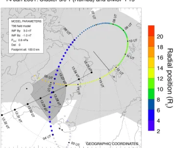
associ-Fig. 2. Ionospheric projection of the Cluster and DMSP F15
or-bit on 14 January 2001. Momentary locations are indicated every 30 min for Cluster and every minute after 13:25 UT for DMSP F15. The altitude of Cluster is given by a colour scale. Also marked are the field-of-views of some SuperDARN radar facilities, the range of the ESR northward pointing radar beam, and the scan coverage of the STF IS-radar. The coordinate grid is geographic.
ated with particle precipitation and ionospheric current flow. We will then inspect the Cluster data from multi-satellite sets of several instruments to investigate the usefulness of three-dimensional measurements in space for the understanding of complex dynamical features.
Since we will use a very large variety of instruments, we prefer not to introduce them in a special section on instru-mentation in order to avoid confusing cross references in the text. Whenever necessary, we will explain the main char-acteristic features of the utilised instrumentation in the text next to the presentation of the observations, and refer to more instrument-specific Cluster publications in this issue, or pub-lications in the Satellite Ground-Based Coordination Source-book (ESA SP1198).
2 Observations
2.1 Interplanetary conditions and overview of some Cluster and ESR observations
On 14 January 2001, from about 07:00 UT onwards, the four Cluster spacecraft passed through the northern mag-netospheric lobe and mantle on their way towards the day-side post-noon magnetopause. In Fig. 1, we show the de-tailed Cluster orbit in the Geocentric Solar Eccliptic (GSE)
XY, XZ and Y Z planes. The dashed and full blue lines indicate a model bow shock and magnetopause at Z, Y ,
X = 0, respectively, and the red and green lines repre-sent field lines connecting to either the southern or northern
Fig. 3a. Overview of the IMF clock angle seen by Cluster FGM
in the magnetosheath after 15:00 UT (blue) in comparison with the IMF clock angle seen by the ACE satellite at 220 REupstream from
10:00 to 24:00 UT on 14 January 2001 (red).
hemisphere ionosphere. We used a standard Tsyganenko-96 model (Tsyganenko, 1995), and chose the input parameters as IMF BY = 3.0 nT, IMF BZ = −1.0 nT, a solar wind pressure of 0.6 nPa and Dst = 0. According to the model, close conjunctions with the ESR and the S¨ondre Str¨omfjord (STF) radars were predicted for 12:00 UT and 15:00 UT, re-spectively, with a final exit into the magnetosheath at around 16:00 UT, corresponding to about 15:00 MLT. In order to allow for a closer inspection of the ground-based data with respect to the Cluster measurements in the following sec-tions, we give in Fig. 2 the consecutive locations for the northern hemisphere magnetic footprints of the Cluster or-bit from 04:00 UT to the expected magnetopause crossing at 16:00 UT. For later reference, we mark in Fig. 2 the location and extent of the ESR field-aligned and northward pointing antenna beams, the scan coverage of the STF radar, and the field-of-views of the SuperDARN radars in the relevant sec-tor. In addition, we mark the orbit footprints of the DMSP F15 satellite during a passage over Greenland from 13:25 to 13:31 UT (see Fig. 24 below for the data from that passage). If we want to interpret the detailed ground-based and Clus-ter data on the background of the prevailing solar wind condi-tions, we require as exact as possible knowledge of the direc-tion and strength of the interplanetary magnetic field (IMF) and the solar wind pressure at the sub-solar magnetosphere. With no near-Earth solar wind monitoring satellite available for this study, we had to rely on measurements by the ACE satellite close to the L1 point, which is more than 220 RE upstream in the solar wind. Using the fact that the solar wind clock angle (the IMF direction in the GSE Y Z-plane) is maintained during the passage of the IMF through the Earth’s bow shock, we have carried out a cross-correlation between the interplanetary magnetic field angle at ACE and the angle of the magnetic field as seen by the Cluster FGM instrument
Fig. 3b. Detailed ACE data, shifted by a time-lag of 75 min as
determined in Fig. 3a, from 12:00 to 14:00 UT on 14 January 2001. (From top to bottom: solar wind dynamic pressure, IMF X, Y and Zcomponents in GSM coordinates, and IMF clock angle).
in the magnetosheath after about 15:00 UT (Balogh et al., 2001, this issue). In Fig. 3a, we show the excellent agree-ment of these two data sets by applying a delay of 75 min between ACE and Cluster when it is in the magnetosheath close to the magnetopause. The delay is very reasonable for a slow solar wind of 350–390 km/s, as observed on 14 Jan-uary 2001.
In Fig. 3b, we show for further reference a more complete set of relevant ACE data for the time interval studied below, now shifted by the lag determined in Fig. 3a. We can con-clude that neither the solar wind pressure (top panel) nor the IMF BZ-component (panel 4) reveal that this period could be particularly interesting for solar wind effects on the magne-tosphere ionosphere system. Apart from a short-lived devi-ation of BZto small or even slightly negative values, which moves the IMF vector into the equatorial plane (so the clock angle is near 90◦, bottom panel), there are no large
indi-cations of solar wind forcing at all. The deviations in the clock angle are associated with negative excursions of the
BY-component (panel 3), and the BX-component (panel 2) is negative throughout the interval.
Using the inferred time shift of 75 min between the solar wind variations seen at ACE and their expected effects on the dayside magnetopause, we can easily understand the basic characteristics of EISCAT ESR and Cluster CIS observations during the entire northern hemisphere orbital portion on 14 January 2001. In Fig. 4, we show in a multipanel presentation the IMF BZcomponent seen at ACE with a delay of 75 mins (top panel), the electron density as seen by the ESR north-ward pointing and field-aligned antennas (panels 4 and 5, respectively), and in the bottom panel, magnetospheric ions as measured by the CIS experiment on Cluster spacecraft 3 (R`eme et al., 2001, this issue). The ESR facility and its data products are described in more detail below. From this figure, a number of observations can readily be made. During the period of primarily southward directed IMF from 07:00 to 11:00 UT, both the field-aligned and northward pointing ESR antennas are passed by frequent poleward moving events of increased ionisation. These events, and in particular those marked in Fig. 4 with a red bar, are studied in detail in a parallel paper by Lockwood et al. (2001a, this issue), who interprete them as signatures of bursty reconnection at a sub-solar neutral line, which, during this period, must map to a location south of the ESR. In addition, during this time pe-riod, it can be concluded that the Cluster spacecraft passes from the relatively empty northern magnetospheric lobe into the plasma mantle, where multiple regions of enhanced ion fluxes pass the spacecraft (see again Lockwood et al., 2001a, this issue, for a more detailed discussion).
At 11:00 UT, the sudden northward turning of the IMF leads to a shrinking of the magnetospheric polar cap which in turn, results in a fast passage of the Cluster spacecraft through the poleward contracting field lines connected to the LLBL and finally reaching a trapped high-energy ion popula-tion, which is typical for the dayside Boundary Plasma Sheet (BPS). After 11:00 UT, the Cluster spacecraft remained most of the time in the BPS region, with the exception of a few shortlived encounters of the Low Latitude Boundary Layer (LLBL) plasma, containing lower energy magnetos-peath ions (see arrows in Fig. 4). Again we have chosen to discuss these multiple encounters of field lines connected to the LLBL by Cluster, and coordinated ground-based obser-vations of associated high-latitude features in a parallel paper (see Lockwood et al., 2001b, this issue).
After the distinct magnetospheric reorganisation occuring at 11:00 UT, even the ionospheric features seen by ESR change in character. The relative absence of electron den-sity structures in the data from the field-aligned ESR beam implies that the open-closed field line boundary must have contracted to polewards of the ESR field line, or that the reconnection line has shifted in longitude such that newly-opened field lines no longer pass over the ESR field line. Furthermore, the still surprisingly frequent poleward moving events in the ionisation, as seen along the northward looking
antenna beam, appear now much slower in their poleward velocity, which is indicative of a decrease in the overall con-vection velocity, as expected for weakly northward IMF.
The next dramatic event occurs at about 13:30 UT, when ESR records a series of poleward moving ionisation features of a rather different character than any of the previous ones. An initial rather broad poleward moving enhancement of the electron density is followed by a sharp channel of decreased ionisation, which is directly followed again by quite a narrow ionisation increase, apparently originating at far lower lati-tudes than any of the previous events (see a higher resolution presentation of this data in Fig. 13). During this transient event at the ESR location, the CIS instrument (located just off the Greenland’s east coast) detects a short-lived but nev-ertheless complete drop out of the trapped high energy BPS plasma simultaneously with large fluxes of magnetosheath ions, a signature typical of the magnetosperic cusp (Smith and Lockwood, 1996). As we will show below, all other in-struments on Cluster see features typical for the magneto-spheric cusp at this moment. The nature of this sudden cusp-like activity at 15:00 MLT, i.e. well away from any expected nominal cusp location, is the main topic for the following comparative study of Cluster and ground-based data.
The final noteworthy observation in Fig. 4 is the exit of the Cluster spacecraft into the magnetosheath at 15:00 UT, i.e. about one hour earlier than predicted by the model, using a standard solar wind parameter set. The ESR observations stop at about this time due to a scheduled end of operation.
2.2 Ground-based observations during the transient cusp event around 13:30 UT
In the following section, we will utilise a complete set of ground-based observations to study the global and meso-scale evolution of magnetospheric convection and iono-spheric current flow, which consequently leads to the surpris-ing event of cusp-like plasma seen by Cluster at 15:00 MLT. The most appropriate ground-based tool to provide a global view of the instantaneous convection pattern and its dynam-ical development is the Super-Dual Auroral Radar Network (SuperDARN, Greenwald et al., 1995), which now employs 4 overlapping radar pairs (i.e. 8 radar facilities) in the north-ern hemisphere, covering the better portion of the northnorth-ern polar cap and auroral zone. In Fig. 5, we show the locations and overlapping fields-of-view of these radars. For further reference, we also indicate in this figure the locations of key magnetometer stations within the CANOPUS (red squares; Hughes et al., 1997), Greenland (light-green squares; http://web.dmi.dk/fsweb/projects/chain/greenland.html) and IMAGE (blue squares; Viljanen and H¨akkinen, 1997) net-works of magnetometers. During the present study, these ar-rays of instruments are located in the dawn, noon, and post-noon sector, respectively. The darker green squares indicate magnetometers in the Russian Arctic, which are not used for this particular study. Note, however, that the IMAGE magne-tometer network is part of the Scandinavian multi-instrument network MIRACLE (Syrj¨asuo et al., 1998) which also
em-83 81 79 77 75 14 January 2001 600 400 200 inv. la titude (deg) hei ght ( km) → cusp sheath LLBL events mantle Dayside BPS lobe LLBL
northward IMF turning
closest ESR/Cluster conj. ACE IMF Bz
Fig. 4. Multipanel overview from 07:00
to 16:00 UT of ACE IMF BZ data
(shifted by 75 min), in direct com-parison with EISCAT ESR measure-ments of the ionospheric electron den-sity along a northpointing (i.e. versus latitude in panel 2) and field-aligned (i.e. versus altitude in panel 3) radar beam, and Cluster CIS data of the ob-served total ion flux on spacecraft 3 (bottom panel). Key events discussed in either this or two companion papers by Lockwood et al. (2001a, b, this is-sue) are marked with a blue, red, and yellow bar, respectively. Plasma fea-tures discussed in the text are labelled with arrows and the northward turning of the IMF at 11:00 UT is marked with a heavy vertical bar.
ploys a bistatic VHF radar and a number of all-sky cameras, the northernmost one of which will be used in association with the ESR data below (see Fig. 13). A similar cover-age of radars and other instruments is achieved at southern high-latitudes (data not used in this study; see Greenwald et al. (1995), and Opgenoorth and Lockwood (1997) for de-tails).
By using the line-of-sight velocities of all 8 individual radar pairs, it is possible to derive a realistic estimate of the global convection flow by fitting the observed flow patterns to a convection model characteristic for the prevailing solar wind conditions (see Ruohoniemi and Baker, 1998, for more details of this method). In Fig. 6 (panels a to h), we show eight selected instantaneous convection flow patterns as de-rived from the data of the northern hemisphere SuperDARN radar network, using information about the solar wind from the ACE spacecraft delayed by 75 min. The clock angle and intensity of the applied IMF is indicated in the small dial at the top right corner of each image. The original data stems
from radar scans of 2 min in duration, which determines the time resolution of these global flow patterns. The velocities shown range from 0 to 1000 m/s, according to a colour scale in the top left corner of each image.
From these images, we see that at 13:22:24 UT the throat of the dayside two-cell convection pattern, the most likely position of the magnetospheric cusp, was located at a pre-noon position over eastern Canada. Northern Greenland and the polar cap north of Svalbard are covered by a broad region of anti-sunward convection, representing the poleward part of the evening sector convection cell. The nightside portion of the morning sector convection cell is located over north-ern Canada and Alaska. Generally, the auroral oval is con-tracted, as could be expected for a northward IMF condition. Two min later, at 13:24:26, a new region of northeastward di-rected flow appears at the nominal cusp location. However, we would like to point out that a very small indication of this new flow is already visible in the first image.
Fig. 5. Northern hemisphere map illustrating the coverage of
Su-perDARN and magnetometer networks used in this study (see text for details). The shaded area is the field-of-view of a radar under construction.
13:32:34 UT), it can be seen how the new flow-channel grows, and finally connects the morning sector auroral oval flow over Canada across the north of Greenland to the post-noon polar cap flow north of the ESR. At 13:34:36 UT it is continuous from eastern Canada to the Arctic Ocean, north of Svalbard, and a strong westward flow-channel develops in the post-noon auroral zone, just to the north of mainland Scandinavia and the northern part of Greenland. Even the eastward directed auroral zone flows over mainland Canada and Alaska are considerably enhanced by this time. The new flow pattern has by now resulted in a peculiar narrow exten-sion of the dusk sector convection cell, which appears very much like a superposition of a new shear-flow pattern on the standard quiet-time convection pattern.
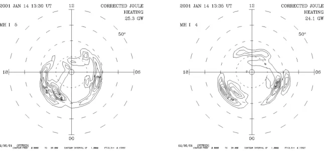
To illustrate the nature of this new intense flow regime, we leave Fig. 6 for a while, and show in Fig. 7a the distribu-tion of Joule heating in the northern hemisphere as calculated with the help of the Assimilative Mapping of Ionospheric Electrodynamics (AMIE, Richmond, 1992; Lu et al., 1997) and in Fig. 7b, the distribution of field-aligned currents at two selected times, namely 13:30 and 13:35 UT. For this study, the AMIE input consisted of data from all the SuperDARN and EISCAR ESR line-of-sight velocities, 4 DMSP satellites (both ion drifts and particles), 4 NOAA satellites (particle data only), and 94 ground-based magnetometers. AMIE pa-rameter maps were derived with 5 min resolution. The first panel of Fig. 7a illustrates the character of the initial long flow-channel across the dayside portions of the two earlier convection cells at 13:30 UT. Only 5 min later, at 13:35 UT, does a second heat- (i.e. flow-) channel develop as an
auro-ral oval return flow. As seen from the SuperDARN data in Fig. 6, its direction is westward and it lies at lower latitudes. The same temporal sequence is apparent from the field-aligned current distribution in Fig. 7b; at 13:30 UT, an ini-tial new pair of field-aligned current sheets appears superim-posed on the weak standard Region I and II currents. The current is directed downward at the poleward side and up-ward at the equatorup-ward side, in order to imbed an east-ward directed flow-channel and a westeast-ward directed iono-spheric current flow (see also magnetometer data in Fig. 9). At 13:35 UT, this field-aligned current pair is more concen-trated at higher latitudes, and a third, downward current sheet has developed equatorwards of the westward flow (eastward ionospheric current)in the post-noon auroral zone.
Returning to Fig. 6, the SuperDARN data shows that after the maximum phase of the transient event at 13:34:36 UT, the eastward directed portion of the new convection channel, i.e. the polar cap part, decays somewhat earlier than the west-ward directed auroral zone flow. After about 13:50 UT, the global convection has returned to a more normal undistorted 2-cell pattern now exhibiting again a clear convection throat over eastern Canada.
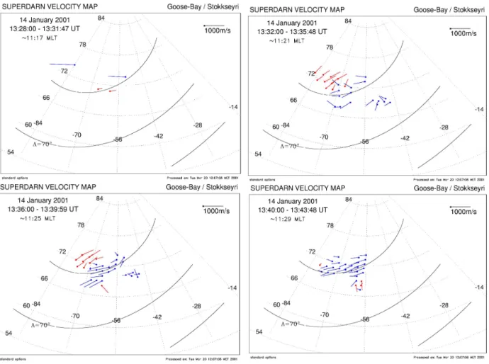
We are well aware of the fact that the data presented in Fig. 6 is quite strongly based on several model assumptions and represents only a best fit restricted by many individual line-of-sight velocity observations and a model convection pattern (Ruohoniemi and Baker, 1998). In order to illustrate that the observations described above are a true pattern seen even in the combined vector maps of individual radar pairs, we show in Fig. 8 data from the Goose Bay / Iceland West (Stockseyri) DARN radar pair. In these spatially limited, but more directly derived vector maps over Greenland, the ear-lier noted development and decay of a short-lived eastward (red vectors) convection flow-channel followed by the later development and decay of a westward (blue vectors) convec-tion flow-channel becomes even more evident. Thus, we con-clude that the data from direct bistatic vector measurements strongly support the content of the global convection maps derived by the method of Ruohoniemi and Baker (1998).
However, the EISCAT data in Fig. 4 clearly indicates a poleward progression of the new electron density feature at 13:30 UT, something that is not quite apparent from these time integrated vector maps and the AMIE model results. In order to further investigate whether SuperDARN data can support these ESR observations, we have inspected data along individual beams of the SuperDARN radars in search of poleward moving signatures (data not shown here). With varying clarity but nevertheless consistently observed in all 5 radars, a new regime of anti-sunward flow (away from the radars) was observed after 13:30 UT, which progressed pole-ward with time until about 14:00 UT.
There is, however, yet another and possibly even more re-liable way of investigating flow enhancement events in the high-latitude dayside ionosphere. As already mentioned in the discussion above, intense flow-channel events are as-sociated with field-aligned currents, electric fields, and last but not least, the precipitation of magnetospheric or
magne-Fig. 6. Panel plot of 8 instances of global ionospheric convection as seen by the SuperDARN network between 13:22 and 13:52 UT on
14 January 2001. The flow vectors represents the fits of the actual line-of-sight velocity observations to a model convection pattern (black full and broken lines represents the electric potential contours), which in turn is constrained by the actual measurements and the solar wind influence on a convection model. The flow velocity is indicated by a colour scale and the derived cross-polar cup potential is given in the top left corner. The IMF data used is time-shifted ACE data (see dial in the top right corner of the images).
Fig. 7a. AMIE model results for two instances (13:30 and 13:35 UT) during the maximum phase of the flow-channel development on 14
January 2001. Global iso-contour patterns of the calculated Joule heating are shown in invariant latitude-MLT frames.
Fig. 7b. Global iso-contour patterns of field-aligned current flow (downward FAC – full contour lines; upward FAC – broken contour lines),
derived using the AMIE technique for the same times and reference frames as Fig. 7a.
tosheath particles into the dayside ionosphere. Therefore, it is obvious that these flow-channels must be associated with ionospheric currents, which in the case of predominant Hall current flow, will be detectable by magnetometer networks as current channels, but with opposite directions, as com-pared to the flow-channels observed by the radars (Stauning, 1995). Indeed, by inspecting magnetic records from high-latitude stations within the CANOPUS Churchill line, the Greenland westcoast line and the IMAGE central meridian from Svalbard to southern Finland, we find that all stations around 13:30 UT are under the influence of alternating east-ward and westeast-ward current flows (original magnetogram data not shown here). In these magnetograms, we find a distinct phase-shift of the peak disturbances with higher and higher latitudes, indicating a poleward progression of the associated
current patterns, which we would like to illustrate in more detail.
In Fig. 9, we display the magnetic X-disturbance mea-sured at the three meridional lines of magnetometers in a colour-coded latitude versus time plot. Red areas indicate eastward current flow and blue (or green) areas indicate west-ward current flow. Following Stauning (1995), we assume that ionospheric Hall currents are the main contributors to dayside high-latitude magnetic disturbances. We find that the blue-green areas are westward currents within the initial eastward flow seen by the radars, while the red areas would correspond to the later development of primarily westward convection flow at lower latitudes. It is striking how well these independent magnetic observations support the radar observations discussed above, but now with the addition of
Fig. 8. Four examples of consecutive direct determinations of the horizontal ionospheric plasma flow from overlapping bi-static line-of-sight
velocity measurements by the Stockseyri/Goosebay SuperDARN radar pair, overlooking the Greenland sector (compare with Fig. 2). The dot marks the origin of the velocity vectors, such that red vectors represent eastward plasma flow and blue vectors represent westward plasma flow.
a new perspective on the meridional motion of the observed feature, which was not as readily resolvable from the presen-tation of the radar data. The central panel of Fig. 9 corre-sponds to a meridian only slightly east of the nominal cusp location where we saw the first appearance of eastward flow in radar data shortly after 13:20 UT. In addition from this data, we see that a new region of westward current flow (east-ward convection flow) appears just after 13:20 UT. It expands first equatorward, but after a few minutes, it expands pole-ward with a velocity of about 1.5 km/s. Not as clear, but in a similar manner, an initial equatorward erosion of pre-existing eastward current flow and later a poleward progres-sion of westward current flow is seen in the CANOPUS data (top panel). In the Scandinavian IMAGE data, the lack of stations between Svalbard and mainland Scandinavia (with the exception of Bj¨orn¨oya, BJN) gives insufficient data cov-erage at the relevant latitude. At 13:30 UT, all three meridian chains record the poleward motion of an eastward current channel (westward flow) which is located equatorward of the first current. The Greenland data show that this poleward ex-pansion ceases at about 13:40 UT, reaching a northernmost
invariant latitude of 80◦. This observed ionospheric current pattern was of course one of the inputs to the AMIE results, yielding the derivation of a triple field-aligned current struc-ture, downward at the poleward and equatorward edges, and upwardly directed in its central portion.
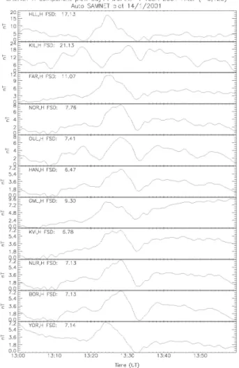
The SAMNET magnetometer network (Yeoman et al., 1990) consists of stations at both auroral and subauroral lat-itudes in the Iceland-UK-Scandinavian sector (see Fig. 10a for a map of SAMNET stations). In particular, data from the subauroral longitudinal line of stations is helpful in identifying the temporal and spatial development of high-latitude phenomena. The distant effects of three-dimensional substorm current wedges and other auroral zone features associated with localised field-aligned current flow create characteristic magnetic disturbances at subauroral latitudes. In Fig. 10b, we show the deflections in the magnetic H -components during the key interval from 13:00–14:00 UT. At the westernmost stations (HLL, FAR, GML, YOR) almost independent of latitude, a positive deflection of the H -component starts to develop just before 13:20 UT, when the first indications of a new flow-channel in the SuperDARN
Fig. 9. Color-coded iso-contour plots of
magnetic X-component disturbance on the ground as determined along mag-netic meridians central to the CANO-PUS (top panel), Greenland (central panel) and IMAGE (bottom panel) magnetometer networks. In these pre-sentations blue areas correspond to westward and red areas to eastward ionospheric current flow.
data over Canada are seen. This initial disturbance declines after 13:28 UT, reaches a minimum at about 13:32 UT, and is followed by a return to positive values by 13:40 UT. Along both sub-auroral longitudinal chains FAR-NOR-OUL and GMI-KVI-NUR-BOR, this initial bipolar feature in the mag-netic H disturbance is seen to propagate eastwards at a rela-tively high velocity (1300 km in about 3 min, corresponding to about 7 km/s). Similar high longitudinal motions of the convection throat during IMF BYchanges have been reported earlier by Greenwald et al. (1995). Along both longitudinal chains, the depth of the negative disturbance increases to-wards the east, indicating a later growth of this disturbance. The propagation of the feature clearly terminates at a longi-tude slightly east of NUR, since there is basically no time shift between NUR and BOR.
Even though this data confirms nicely the fast eastward propagation of a transient high-latitude event, its interpreta-tion in terms of field-aligned current effects is very difficult. We have seen from the AMIE data that the new flow-channel is imbedded between two field-aligned current sheets,
ex-panding towards the east, with the additional complication of the delayed formation (probably not expansion) of a more equatorward located downward directed current. It is clear that SAMNET must record the effects of this complicated development, but further conclusions will require a more de-tailed model analysis of the data, which is beyond the scope of this paper.
From Fig. 2, it becomes evident that at 13:30 UT both the US incoherent scatter radar at S¨ondre Str¨omfjord (STF, Kelly et al., 1995) and the EISCAT Svalbard Radar (ESR, McCrea and Lockwood, 1997) were in excellent locations to provide detailed observations of the different phases of the transient flow event. During this event, the STF radar was operated in a special mode, designed for coordinated ob-servations with the ESR in conjunction with Cluster. This mode consists of an azimuthal scan at constant low eleva-tion towards the northeast of the radar. In the top panel of Fig. 11, we display an overview presentation of the mea-sured line-of-sight velocities during the entire period in ques-tion, together with more detailed line-of-sight velocities (left
1380 H. J. Opgenoorth et al.: Cluster and ground-based observations of a transient cusp event
Fig. 10a. Map of stations in the SAMNET sub-auroral
magnetome-ter array.
3 panels) and associated ion temperatures (right 3 panels) from three consecutive scans during the key interval from 13:28 to 13:39 UT. The scan duration is slightly more than 4 min and the scans are continuous, i. e. a scan towards lower latitudes (top two panels) is directly followed by a re-turn scan towards higher latitudes (central two panels), and then equatorward again (bottom two panels). More infor-mation on this special mode of operation can be found at http://isr.sri.com/iono/cluster/cluster experiments.html.
Already in the relatively coarse overview data in the top panel of Fig. 11, one can clearly identify the short-lived event of anti-sunward flow shortly after 13:30 UT (blue = away from the radar), which we have identified in all other data sets so far. Note that even though the axis is labelled as alti-tude, the main effects along that axis will be due to latitude variations, as the beam is pointed towards north and north-east at a low elevation. The detailed scans shown in the left lower panels of Fig. 11 illustrate that the flow event is re-stricted to the north-pointing directions of the scans, and that it is indeed very short-lived at this location. Some initial in-dications may be found in the first scan starting at 13:28 UT, and the flow-channel is fully developed when the second scan reaches this position again at 13:35 UT (i.e. close to the end time of this poleward turning azimuthal scan). The next re-turn scan, passing that same region at 13:37 UT, already sees a clear decay. The same feature becomes visible in the right lower panels of Fig. 11, displaying the ion temperature along the radar beam. It is well-known from numerous incoherent scatter radar studies that short-lived flow enhancements have a pronounced effect on the temperature of the ionospheric ion population through the drastically increased ion neutral collisional heating. In the ion temperature data it is clear that not only the transient nature of the event stands out, but also comparing the lower two panels to the right, its poleward motion can be seen.
Fig. 10b. Horizontal component magnetograms from the SAMNET
network, sorted from top to bottom along three longitudinal profiles at different latitudes (HLL–KIL, FAR–OUL, and GML–BOR).
This portion of the scan area of the STF radar was about 45◦in longitude to the west of the nominal Cluster footprint at that particular time, and about 30◦to the east of the lo-cation of the initial flow-channel, as seen by SuperDARN over Canada at 13:20 UT. At the same time, the northward pointing antenna beam of the ESR is only 15◦to the east and probably a few degrees to the north of the Cluster footprint (see Fig. 2, and discussion below). A spatial and temporal connection between the observations at these two key radar systems is provided by a Norwegian all-sky imager, located in Ny ˚Alesund. This camera is sensitive to red auroral emis-sions of 630.0 nm. In Fig. 12, we show three selected images of red-line aurora, projected onto a map with the assumption of a central emission at an altitude of 250 km. A more detail discussion of this optical data with respect to selected Clus-ter and low altitude satellite data is presented by Moen et al. (2001, this issue). The auroral data nicely illustrate how the features which were observed in the STF scan around 13:35 UT expand primarily eastward, but even slightly pole-ward, past the nominal location of the Cluster footprint at
Fig. 11. Top panel: overview presentation of STF line-of-sight measurements along an azimuthal scan in the northeastern quadrant, plotted
versus altitude and time (blue vectors represent flow away from the radar and red vectors represent flow towards). Bottom left panels: line-of sight plasma velocity measurements (red=away) for three consecutive scans from 13:28–13:47. Bottom right panels: ion temperature measurements (red=high Ti) for three consecutive scans from 13:28–13:47. North is to the top of the scan plots and east to the right.
1382 H. J. Opgenoorth et al.: Cluster and ground-based observations of a transient cusp event
Fig. 12. Three selected all-sky camera images in 630.0 nm emissions from the Norwegian camera at NAL. The relevant portion of the
projected Cluster orbit is indicated in the images (see time marks in the first image).
13:34 UT and into the vicinity of Svalbard at about 13:38 UT. By comparing the first and second images in Fig. 12, one re-alises that Cluster should have been affected by the auroral expansion at about 13:30–13:34 UT (see Moen et al., 2001, this issue, for more auroral images and also the following discussion in Sect. 2.3 for detailed Cluster data). The ESR should see the first effects somewhat delayed, i.e. after about 13:40 UT (see last image at 13:38 UT and the discussion be-low).
Detailed ESR data of electron density (the same data as in Fig. 4, top panel, but with a higher resolution) and ion tem-perature (the latter as a proxy of enhanced ionospheric flow) are presented in Fig. 13. In this data, the poleward moving character of the transient flow event is again obvious. The sharpest feature seen by the ESR is a poleward propagating depletion of the electron density (blue area at 13:40 UT in the top panel), coinciding with a region of enhanced ion temper-atures, indicating enhanced plasma flow velocity (red/yellow area in the second panel). In the full set of ESR data (data not shown here), one can see that the ion flow direction in this channel of higher temperature is clearly away from the radar. We conclude that this sharp feature must be charac-teristic for the flow-channel itself. It is directly followed by an adjacent propagating region of enhanced ionisation (red narrow structure around 13:50 UT), originating at notably a lower latitude than any other electron density feature seen by the ESR during the entire Cluster passage (see also Fig. 4). We believe that it is created by new and more energetic pre-cipitation, therefore affecting a lower altitude portion of the obliquely northward pointing ESR beam. In order to support this conclusion, we present in the bottom panel of Fig. 13 an optical keogram from the Italian all-sky camera (ITACA) at Ny ˚Alesund (i.e. 557.7 nm emissions along a meridional profile plotted versus latitude and time with the assumption of a central emission altitude at 110 km). ITACA is part of the MIRACLE network. The heavy black line in the
bot-tom panel of Fig. 13 corresponds to the lowest latitude in the data from the ESR oblique beam. By continuing the slope of the poleward propagating auroral forms in the keogram to that particular latitude (thin lines), one can readily associate the main flow-channel in the ESR data with a region void of auroral emissions (label 1). The channel of precipitation at 13:50 UT is associated with discrete 557.7 nm aurora (la-bel 2). The fact that the aurora is green, i.e. resulting from particle precipition to altitudes of 110–130 km, explains the ESR observations of increased electron densities at lower al-titudes. Apart from this main event, the existence of a sec-ond pair of events is revealed in the combined presentation in Fig. 13. A weaker flow-channel (as recognised by the cav-ity in ne, enhanced Ti and a region void of aurora (label 3)) exhibiting only limited poleward expansion is followed by a region of enhanced precipitation and auroral emissions (la-bel 4). This second sequence of events is actually apparent in detailed Cluster data as well and will be discussed below in more detail.
In finishing this comprehensive discussion of ground-based data sets, we note that the clear poleward mov-ing events start at the lowest ranges of the radar at about 13:40 UT, i. e. somewhat after the onset of the poleward mo-tion of currents and radar-echoes seen by other ground-based instruments (see Fig. 9) and the sudden onset of cusp-like precipitation in the Cluster data (Fig. 4 and discussion be-low). Furthermore, we note that the poleward velocity of about 0.5 km/s derived for the flow-channel and the adjacent region of enhanced electron density events seen by the ESR is much slower than the poleward velocity of about 1.5 km/s derived for the magnetic features seen at latitudes of the IM-AGE chain between 13:30 and 13:40 UT.
In order to associate the features seen by the ESR radar with the magnetic features monitored by the IMAGE chain of magnetometers, we present the two data sets in a com-bined stacked plot in Fig. 14. When analysing Fig. 14, one
1 2 3 4
Fig. 13. Comparison of EISCAT ESR
data versus latitude and time of elec-tron density (top panel) and ion tem-perature (central panel) with a keogram from optical observations of 557.7 nm emissions by the Itaca all-sky camera, located just to the south of the range of the ESR poleward pointing beam. The heavy black line in the keogram marks the lowest latitude in the ESR data, and the thin arrows are guidelines to con-nect the regions void or filled with au-rora to corresponding regions of low and high electron density (respectively, high and low ion temperature) in the ESR data.
needs to keep in mind that the lowest latitude data in the pole-ward pointing ESR beam (77.9◦ Inv. Lat. in the top panel) is about 200 km to the north of the highest latitude data in the IMAGE chain (76.7◦Inv. Lat. in the bottom panel). The insert of Cluster CIS data in the central panel should be ig-nored for the time being, as it will be discussed in Sect. 2.3 below. Slanted and vertical lines in this stacked presentation are meant to assist the eye in connecting the key features of the various data. Obviously, the initial broad and fluctuating eastward current is associated with a similarly broad region of enhanced (and fluctuating) electron density in the ESR data. In correspondence to the earlier comparisons of coher-ent radar and magnetometer observations the flow-channel at ESR (decreased ne) was associated at that time with a nar-row region of westward current flow in the IMAGE data and a main precipitation region (enhanced ne) with a new narrow
eastward current, etc. for the second set of transients. A comparison of Fig. 14 with Fig. 9 increases the con-fidence in this interpretation of physically associated fea-tures. Both in Canada and over Greenland, the initially fast poleward expansion of transient current channels around 13:30 UT decreased considerably after reaching about 80◦ invariant latitude. In Fig. 14, this latitudinal boundary is lo-cated just poleward of the IMAGE chain, but right in the vicinity of the northward pointing ESR radar beam. Thus, the difference in the observed poleward velocity in the IM-AGE and ESR data is explained by a global pattern that is not visible in the individual data sets. However, the observed features match very well.
In this section, we have presented data from a large net-work of ground-based stations to infer the dynamics of the ionospheric convection and several associated transient
fea-13:00 UT 14:00
nT
13:00 13:30
EISCAT ESR Electron Density
Cluster CIS s/c 3, Ion data
IMAGE X-Component 14:00
Fig. 14. Stacked plot of ESR electron density along the northward pointing radar beam (top panel, as in Fig. 13), total ion flux data from the
CIS instrument on Cluster spacecraft 3, and the magnetic X-component disturbance along the central meridian of the IMAGE magnetometer array, ranging from southern Finland to just southward of the latitude of the ESR measurement range along the poleward pointing beam. The thin arrows mark the relation between features in the CIS ion data with regions of eastward (red) and westward (green) current flow in the magnetometer data. Heavier bars illustrate the possible continuation of the poleward propagation of these features towards the southernmost latitude of the ESR.
tures between 13:20 and 13:40 UT. In summary, we can state that a new eastward directed flow-channel, originating over Canada at about 13:20 UT, expanded during the following 20 min both eastwards and polewards, and finally reached the latitude and longitude of Svalbard at 13:35 UT. The change in the global pattern is best recognised in the data of the Su-perDARN network, supported by the AMIE model. In more detail, the poleward motion of this eastward directed flow-channel was clearly detected in meridionally directed radar beams or individual magnetometer chains, and the eastward motion was confirmed not only by the use of data along
sev-eral meridians, but also by an additional well positioned all-sky camera and lower-latitude magnetometers. From the en-tity of these data sets we conclude that the predicted footprint of the Cluster satellites was engulfed by the leading north-eastern edge of this new expanding flow-channel at about 13:30 UT. During the following interval of 20–30 min, Clus-ter remained to the west of Svalbard, at a comparable mag-netic latitude with a fair possiblity to observe transient con-vection changes a few minutes before they affected the Sval-bard region.
Fig. 15. CIS data on Cluster spacecraft 3 from 13:00 to 14:00 UT on 14 Janaury 2001, showing the bulk ion velocity in three components
(top panel), the pitch angle distribution of ions in the 3.8–28 keV energy range (central panel), and the total ion flux versus energy and time (bottom panel).
Fig. 16. CIS data of the total ion fluxes versus energy for Cluster spacecraft 1, 3, and 4, illustrating the variations between spacecraft 1, 3 and
2.3 Cluster observations during the transient cusp en-counter around 13:30 UT
Figure 4 already gives an indication of the similarity of the transient features as seen by the ESR and the Cluster CIS in-strument. Figure 14, shows the ESR (top panel) and CIS data (central panel), at much higher time resolutions than Fig. 4, concentrating on the hour of interest between 13:00 and 14:00 UT. In order to bridge the latitudinal gap between the ESR data and Cluster (just as the all-sky camera data in Fig. 13 bridged the gap between Greenland, Cluster, and Svalbard) we add in the bottom panel once more the data from the IMAGE magnetometer chain. With the aid of ver-tical lines, Fig. 14 illustrates that during the time interval from 13:30 to 13:50 UT, Cluster must have been passed al-most simultaneously by the same structures of convection and precipitation, which passed over the magnetometers at the latitude of Svalbard. With a delay of the order of 10 min, the same structures are seen to propagate into the northward looking ESR radar beam where they are observed to continue their propagation towards about 80◦ invariant latitude (see detailed discussion above). The combined data also clearly shows that the main cusp-like features in the CIS data are as-sociated with the first arrival of the eastward flow-channel. However, a careful inspection of the combined data reveals fine structure in the ion data, which might be associated with a second, but minor surge of cusp-like features at around 13:40 to 13:45 UT. As in the main event, its ionospheric features are a decrease in eastward current flow (westward electrojet or enhanced eastward plasma flow) and a depletion in electron density, which is indicative of a flow-channel (see also a clear second enhancement of Tiin Fig. 13 at that time). More detailed CIS data from spacecraft 3 in Fig. 15 shows the three-component H+ velocities (top panel), the pitch-angle distribution of trapped magnetospheric ions in the energy range of 3.8–30 keV (central panel) and the stan-dard total ion flux for reference (bottom panel). The cen-tral panel illustrates in more detail the complete drop out of magnetosheric particles at the time of arrival of the eastward flow-channel. The second partial drop out from 13:40:46 UT is also clearly contrasted from the time inter-vals of 13:33:40 UT and 13:46:56 UT, when the CIS in-strument observes a mixture of magnetosheath and (some-what depleted) magnetospheric ions. This must mean that the satellites are after the main event located in the magneto-spheric boundary layer adjacent to the main body of the tran-sient structure. The velocity data in the top panel show that CIS, probably as early as 13:26 UT, has entered the vicinity of the cusp region, detecting an enhanced, transient flow in anti-sunward direction. The curves indicate a flow primarily in the −X (i. e. earthward) and +Y (i.e. eastward) direc-tion with a bulk flow velocity of up to 200 km/s. This flow event is observed until 13:37 UT, and is in agreement with the ground-based observation in the vicinity of the Cluster footprint. Successive fine-scale transients are superimposed on the average bulk flow. A diminution of flow can be ob-served around 13:32:33 UT, just adjacent to the main feature
Spacecraft Configuration –
14 January 2001
Electric Field (GSE X) – No Timeshift Timeshift Applied
Fig. 17. Top panel: plot of the Cluster satellite constellation and
the bundle of field lines that they are observing, as modelled by the Cluster orbit visualisation tool; left bottom panel: high res-olution EFW data between 13:29:20 and 13:30:30 UT showing a transient in the total electric field measurements on all four Cluster spacecraft, and right bottom panel: the same EFW data but time-shifted according to a feature passing the satellites with a velocity of vx = −84, vy = −6 and vz = −38 km/sec. The OVT
colour-coding of the satellites and the data is red, green, yellow, and mag-neta for spacecraft 1, 2, 3 and 4, respectively.
in the cusp-like ions. Even though we note that it is very dif-ficult to map velocities from the magnetopause to the iono-sphere along very distorted field lines, it is, nevertheless, in-teresting to note that this anti-sunward, duskward flow would correspond to an ionospheric convective flow of the order of
≤ 1 km/s, primarily eastward in direction, but with a clear poleward component.
So far we have presented Cluster data from only one satel-lite. The use of the full multi-satellite concept of Cluster should allow us to further understand the observed features as effects of a localised propagating magnetospheric struc-ture. In Fig. 16, we show H+ion flux data from all three CIS instruments for the time interval from 13:00 to 14:20 UT (as described in more detail by R`eme et al. (2001, this issue), the CIS experiment on spacecraft 2 suffers from a partial mal-function). In this resolution, the ion data of spacecraft 1 and