Real time degradation identification of UAV using machine learning techniques

HAL Id: hal-01629680

https://hal.archives-ouvertes.fr/hal-01629680

Submitted on 20 Nov 2017

HAL is a multi-disciplinary open access

archive for the deposit and dissemination of

sci-entific research documents, whether they are

pub-lished or not. The documents may come from

teaching and research institutions in France or

abroad, or from public or private research centers.

L’archive ouverte pluridisciplinaire HAL, est

destinée au dépôt et à la diffusion de documents

scientifiques de niveau recherche, publiés ou non,

émanant des établissements d’enseignement et de

recherche français ou étrangers, des laboratoires

publics ou privés.

Real time degradation identification of UAV using

machine learning techniques

Anush Manukyan, Olivares-Mendez Miguel, Holger Voos, Matthieu Geist

To cite this version:

Anush Manukyan, Olivares-Mendez Miguel, Holger Voos, Matthieu Geist. Real time degradation

identification of UAV using machine learning techniques. International Conference on Unmanned

Aircraft Systems (ICUAS), 2017, Miami, United States. �hal-01629680�

Real time degradation identification of UAV using machine learning

techniques

Anush Manukyan

, Miguel A. Olivares-Mendez

, Holger Voos

, Matthieu Geist

∗ University of Luxembourg, Luxembourg

forename.lastname@uni.lu

1 Universit´e de Lorraine, LORIA, UMR 7503, Vandoeuvre-l`es-Nancy, F-54506, France

2 CNRS, LORIA, UMR 7503, Vandoeuvre-l`es-Nancy, F-54506, France

3 LORIA, CentraleSup´elec, Universit´e Paris-Saclay, 57070 Metz, France

forename.lastname@centralesupelec.fr

Abstract— The usages and functionalities of Unmanned Aerial Vehicles (UAV) have grown rapidly during the last years. They are being engaged in many types of missions, ranging from military to agriculture passing by entertainment and rescue or even delivery. Nonetheless, for being able to perform such tasks, UAVs have to navigate safely in an often dynamic and partly unknown environment. This brings many challenges to overcome, some of which can lead to damages or degradations of different body parts. Thus, new tools and methods are required to allow the successful analysis and identification of the different threats that UAVs have to manage during their missions or flights. Various approaches, addressing this domain, have been proposed. However, most of them typically identify the changes in the UAVs behavior rather than the issue. This work presents an approach, which focuses not only on identifying degradations of UAVs during flights, but estimate the source of the failure as well.

I. INTRODUCTION

During last years, the use of intelligent robots in daily ap-plications has grown dramatically and are typically used for performing tasks that are hazardous, dangerous or unpleasant for humans [12]. However, performing such challenging tasks in an unknown and dynamic environment can lead to unexpected events, such as damaging of robots body parts.

To avoid worsening the situations, the robot needs to have knowledge about its own possible damages or defects. These degradations should be detected quickly in order to be able to take an immediate decision during the robots mission. This improves the autonomy of the robot, provides more reliable and safe accomplishment of the task and reduces the risk of unexpected breakdowns [17][20]. In this work, we present a lightweight method that can detect any degradation and point out the cause for the abnormal behavior in real time. Based on a UAVs internal and/or external sensors, the flight data stream is used for analysis and estimation of the UAVs performance using well-known machine learning techniques.

The proposed method consists of two phases: offline learning and online prediction. During the first phase, the training data is processed and prepared such that the model can be trained using a supervised learning approach. The second phase uses the trained model in an online mode and

predicts the level of degradation of the UAV in real time using a sliding time window technique. The model is based on k Nearest Neighbor (kNN) algorithm using Dynamic Time Warping (DTW) as a distance measure. The choice of those algorithms is motivated by the significant results that have been presented in our previous work [14], where we were dealing with the task of identifying anomalies of a UAV in an offline mode exclusively.

This work shows significant improvements of the classifier, not only in terms of accuracy but also in terms of speed and parallelization possibilities, over the previous method [14]. As a proof a concept, a Python based command line tool has been implemented, which provides an interface to analyze data of UAVs, creates and trains models and finally, simulates real time prediction of degradations.

The paper is organized as follows: Section 2 investigates the existing approaches for similar problems. Section 3 describes the fundamental steps of the approach, by giving a detailed explanation about the learning phase and the real time prediction phase. In section 4 we discuss about the experimental setup and the experiments performed for gathering the training data. Then, section 5 presents all the results of the algorithm’s performance evaluations. Finally, section 6 concludes the presented along with the feasible future work.

II. RELATED WORK

Real time anomaly detection of Unmanned Vehicles (UV) has become an extensive research area for fields such as robotic, machine learning, and artificial intelligence. This section first investigates existing approaches for anomaly detection of UVs, and then, reviews the state of the art focused on streaming time series classification.

Afridi et al. [7] implemented a machine learning tool for detecting Anomalies due to Wind Gusts (AWG). AWG accurately detects the wind gust anomalies in the altitude control unit of an Aerosonde UAV. The approach is based on supervised learning using several classification algorithms, based on the Waikato Environment for Knowledge Analysis

(WEKA) implementation, for comparing results. Finally, they show that the J48 decision tree over neural networks algorithms gives the best results. Larrauri et al. [5] designed a novel fully automatic system for overhead power line inspection for UAVs. It enables anomalies detection without requiring manual intervention on the ground station or control center. The main idea is to process the telemetry data and consecutive images sent from the autopilot in order to identify online areas of vegetation, trees and buildings close to power lines and to calculate the distance between power lines and the respective obstacles. They use artificial vision algorithms to calculate distances and detect hotspots. In several research works, Mahanalobis distance is applied as anomaly detection identifier. Such approach is presented by Khalastchi et al. [8] in their online data-driven anomaly detection work for light-weight robots. They show that, for robots and agents, considering the differential of the sensor data instead of the raw data, can improve the anomaly detection process. They use Mahanalobis distance as a distance measure function between simple points and multi-dimensional distributions. In general, the data produced by robots is composed of high-dimensional sensor data, which is not trivial. Therefore, they apply an approach presented in their previous work [2], which focuses on finding the correlation between the attributes in order to reduce the dimensions. Afterwards, they apply Mahalanobis distance, which returns the degree of difference between sets of data being anomalous, and by beforehand-defined threshold, they declare anomalies. Brotherton et al. [6] present another technique of anomaly detection for military aircraft subsystem data. Using Mahanalobis distance they identify whether each individual signal received from an aircraft has normal or abnormal behavior. A similar approach has been presented by Laurikkala et al. [9]. In that case, Mahanalobis distance is used to reduce the multivariate observation to univariate scalars.

Plagemann et al. [4] presents an efficient method for failure detection of mobile robots using mixed-abstraction particle filters [4]. The approach focuses on estimating the failures caused by external influences like collisions or wheel slip. They propose to build a model abstraction hierarchy, which can be used by the mixed-abstraction particle filter algorithm to detect computational resources for the most efficient model whose assumptions are met. This gives the advantage to minimize the computational load while maximizing the soundness of the system. Stavrou et al. [3] introduce a model-based online fault detection and identification approach for service mobile robots, such as iRobot Roomba [22]. The approach of the observer is to track the error between the normal robot dynamics and an estimation based on sensor readings. When changes in the robot behavior are identified, the bounds are used to generate an adaptive threshold, which is considered as a limit of the estimation error. Faults are detected when the estimation error exceeds the threshold. The magnitude of the fault they identified online provides important information about the

severity of the fault. They believe that their approach can be applied to any two-wheeled mobile robot [3][19]. Pokrajac et al. [10] proposed in their study an incremental local outlier detection algorithm for data streams, based on the computation of local neighborhoods densities. The method assigns a degree called local outlier factor (LOF) to each data record. Data records with a high LOF represent a stronger outlier than those with lower LOF. As the first step, the algorithm computes the distance of a data record with all other kth _{nearest neighbors using Euclidean distance.}

Then it computes local reachability density (LRD) of data records as the inverse of the average reachability distance based on the k nearest neighbors of the data record. Finally, it computes LOF of data records as the ratio of the average local reachability density of k nearest neighbors and local reachability density of the data record. At the end, they showed that their algorithm successfully detects outliers with respect to density of their neighboring data records. Another approach for online data stream anomaly detection is presented by Laxhammar et al. [11]. They proposed a parameter-light algorithm, called Sequential Hausdorff Nearest-Neighbor Conformal Anomaly Detector (SHNN-CAD), for sequential anomaly detection in trajectories. The proposed approach is based on adjusting the anomaly threshold in real time. They investigate the performance of SHNN-CAD on four different labeled trajectory datasets, and concluded their investigation by showing a competitive classification performance during unsupervised online learning.

Various other approaches for UV anomaly detection problem have been proposed, however they typically detect anomalies by investigating if there were any changes in the normal behavior or not. Only a few approaches [4], [8], [10] were focusing on anomaly detection in an online mode. Thus, this work presents an additional approach which can both, identify anomalies of UAVs, and pinpoint the exact source of the failure, such as propeller, motor, battery, etc.

III. SLIDING TIME WINDOW DEGRADATION IDENTIFICATION APPROACH

The approach for real time degradation identification, proposed in this paper, consists of two phases: 1) offline model learning and 2) real time prediction using a learnt (trained) model. It focuses on a scenario where the UAV has been given a pre-determined path that it must follow autonomously.

A. Sliding Time Window-Based Model

In the first phase, the model is being trained using a dataset of the UAVs past flights. As the model aims to pinpoint not only degradations but also the exact source of their appearance, the data used for model learning is constructed not only from samples of fault-free flights, but also from samples of flights where UAV had a different

level of degradations.

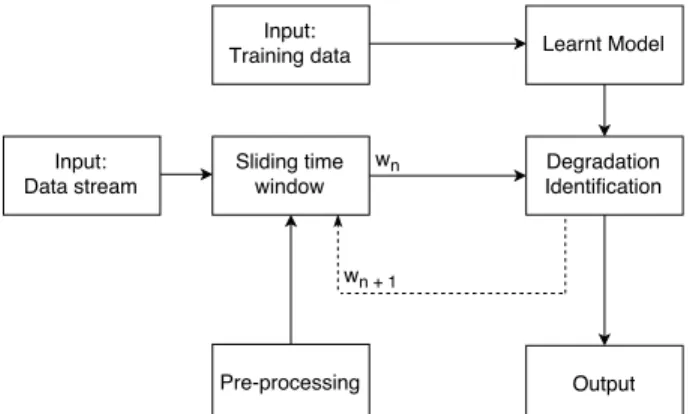
In a model that is not window-based, each flight would have one label, that describes the level of degradation of the flight, and each prediction is made by using the entire flight [14]. However, in a window-based approach, we are working with chunks of flights. Here, we use time windows, meaning that the flights have been split into chunks of constant time intervals. For example, a 1 min flight could have 10 chunks of 6 seconds each. Since chunks of flights are used, instead of having one label describing the entire flight, each time window has its own label. In this way, we can also achieve a more precise labelling of the entire flight. Figure 1 represents the general flow of the model learning process using sliding time window.

Fig. 1: General flow of the model learning using time window.

Once the data is labelled, the model is trained and vali-dated offline in order to find the best parameters to run the model in real time. Since the model uses the labelled time window data, it must simulate the stream of data as well. In this time window-based approach, the simulation restricts the model to only access the current time window for every flight. Thus, it is not allowed to use past or future data points, outside of the current time interval.

Fig. 2: General flow of the real time degradation identifica-tion process.

B. Real Time Prediction Using Sliding Time Window Now, when the model has been trained offline, it can be used online to identify degradations of the UAV in real

time. During the mission of the UAV, flight data is being recorded by internal and/or external sensors and the data is streamed to the degradations identification algorithm, which should be running on a server in the cloud. Running the online model onboard the UAV is also possible, but requires a UAV with a more computing power and thus more battery life.

As data come in, the current time window is filled. In this approach, we use a window-based on duration and not based on the amount of data. This means that after a fixed time interval (e.g., 10 seconds) the current window is closed and sent asynchronously to the machine learning algorithm, which then estimates the behavior of the UAV for the given window. Since we are working on a continuous stream of data, the algorithm predicts the level of degradations in the background while the server already records the incoming stream of data for the next time window. Figure 2 presents each step of degradation identification process in a real time, using offline trained model.

The real time prediction capabilities depend on the amount of data to process for each window and the speed of the prediction algorithm. Because the prediction is run once on each time window, the estimated level of degradation can only be updated every x seconds, x being the size of the time window. Ideally, the computation of the prediction should be fast enough that it yields an estimation before the next time window is reached.

It is worth mentioning, that the streamed data arrives in a raw, unprocessed format, and can contain many unnecessary feature attributes and/or many repetitive data points. This is especially the case when the data is being streamed by high-performance sensors. Therefore, the stream of data should go through some kind of pre-processing. One approach is to pre-process the outgoing stream form the perspective of the UAV. This can be achieved by reducing the frequency of the streamed data. Another way consists of recording the entire stream and only pre-processing the current time window before running the the prediction. The aim of pre-processing the stream is to apply several feature extraction techniques in order to reduce the dimensions of the data and facilitate the next computational steps.

C. Real Time Degradation Identification Process

Following the general model descriptions and learning, this section focuses on the core algorithms and techniques that are used and which have been implemented as a proof of concept on real UAV flights. The classification technique that has been developed in this study is chosen based on the experience of the previous work, where we have learnt that kNN can achieve high-performance results for time series classification. However, the current technique differs from the previous approach by using a sliding window technique, which works with small batches of flight data. Additionally, the calculations of the classifier algorithm have been paral-lelized. The combination of both dramatically decreased the computation time.

The main advantage of kNN is its flexability, that allows the distance measure functions to be easily adapted to the data specificities, in this case to the different lengths of time series. Thus, the Dynamic Time Warping (DTW) has been selected, which computes the best possible alignment warp between two unequal length time series by selecting the one with the minimum value [13][16].

Upcoming is an in-depth explanation of kNN and DTW algorithms.

k Nearest Neighbours Classification Algorithm

At the core, kNN takes a set of labelled training samples and classifies test samples by the use of a similarity or distance metric. In other words, it predicts the label of new objects based on the k most similar training samples, better referred to as k nearest neighbours [1][16][21].

Given a training set X, of size N with Y class labels and an unknown test sample x, the computational steps of kNN are as follows:

• Step1: Choose a k, the number of nearest neighbours. • Step2: Compute the distance d between the test sample

and each training samples, noted d(Xi, x), i∈ [1, n]. • Step3: Sort the distances and extract the class labels

yj, for the smallest jthdistances (j∈ [1, k]).

• Step4: Compute a majority vote on the extracted labels and return the resulting winner, y0.

The majority voting rule assigns the class label to an unknown data object based on the most frequent labels among the k candidates extracted from the training set.

The majority voting formula is the following: y0 = argmax

v

P_{I (v = y}

j), where v is a class label,

yj is the class label for the jth nearest neighbour, and

I (_{·) is an indicator function that returns the value 1 if its} argument is true and 0 otherwise [1].

Dynamic Time Warping

Dynamic Time Warping (DTW) is an algorithm to measure the distance of two time series, or temporal sequences, of different length. It is often compared with the Euclidean distance, which differs in a sense that it only measures the distance between two points, rather than two sets of data of different sizes.

Given two time series X = (x1, x2, ...xN), N ∈ N and

Y = (y1, y2, ...yM), M ∈ N, sampled at unequidistant points

in time. The more similar X and Y are, the smaller the distance function D(X, Y ) is. Furthermore, the value of distance measure function increases as the time series differ more from each other [16].

In other words, the D(X, Y ) is a distance measure function which computes the best possible alignment or the minimum mapping distance between two time series, using dynamic programming approach.

It builds the warping path between time series and returns the distance value by following these tree main conditions:

Boundary condition. The first and last elements of X and Y must map exactly to the starting, respectively ending points of the warping path: p1 = (1, 1) and

pK = (N, M )

Monotonicity condition. Elements of X and Y should stay to time-ordered: n1 ≤ n2 ≤ ... ≤ nK and m1≤

m2≤ ... ≤ mK

Step size condition. While mapping sequences, this condition is used for limiting the warping path from long jumps: pl+1− pl∈ {(1, 1) , (1, 0) , (0, 1)} .

We note p∗, the best warping path between X and Y with the minimal total cost: p∗= argmin(D(X, Y )). This minimization problem is computationally difficult, since the algorithm has to calculate all possible warping paths, which number grows exponentially as the size of the time series grows linearly. Therefore, DTW uses a Dynamic Programming algorithm to find this minimum-distance warp path, which evaluates the recurrence of the cumulative distance that is found in the adjacent elements: Once

D(i,j) = d(xi, yj) + min      D(i, j− 1) D(i− 1, j) D(i− 1, j − 1)

the cumulative distance matrix is computed, we can use backtracking to find the minimum warping path. The last element of the warping path is the distance between two time series [15]. This matrix has complexity of O(M N ), thus in our implementation we decreased the complexity by limiting the warping window size. For the proof of concept those algorithms has been implemented. In the section 5 the evaluation of the algorithms behavior is discussed in a great details.

IV. EXPERIMENTAL SETUP

The used dataset originates from a scenario described in our previous work [14]. The full scenario, or mission, took place indoor, where a motion capture system (OptiTrack) has been setup. A commercially available drone (Ar.Drone), shown on figure 3, has been used and it has been programmed to autonomously follow a pre-defined path. The scenario lasts for about 1m40s, during which time the UAV performs different fast and slow basic maneuvers such as take off, landing, forward/backward moves, right/left turns and hovering.

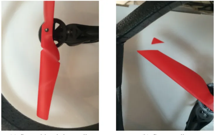
Since the interest of this work is to identify the degradations of a UAVs body parts, the propellers have been chosen as the main target for being altered and damaged. Several incremental damages, such as bending, cutting and/or scraping has been made on the propellers. At each level of damage, the scenario has been fully run in order to observe and collect the flight data. Figure 4 presents the

different kind of damages that have been made on the UAVs propellers. Even though this paper focuses on degradations of propellers, the same technique can be applied for any other body parts of the UAV, such as motors or batteries.

Experiments have been video recorded and one of the experiments is available online [23], which showcases the desired flight against the “Worst” flight.

Fig. 3: A commercially available drone (Ar.Drone)

(a) Cut and bended propeller. (b) Cut propeller.

Fig. 4: Different damages made on propellers.

V. EVALUATIONS AND RESULTS

In this section, we introduce the dataset used for the evaluation. Then, we describe in detail the real time data stream simulation for labeling, pre-processing and model learning. After, we present the evaluations of several models, along with the comparison of the results from the previous work [14].

A. Data

The data used in this research is based on 50 flights performed by a commercially available “AR.Drone” UAV. Each flight has been recorded by the UAVs internal sensors, which contain up to 36 different attributes such as position, speed, battery percentage or even rotation. Because the scenario was played in a small environment, it has also been possible to record the flight using an external high

performance motion capture system, allowing to record the precise location coordinates of the UAV at a rate of 240 readings per second. In this paper, the data gathered form the motion capture system has been used, due to its preciseness.

Once the data has been gathered, pre-processing is directly applied by removing consecutive location points that are less than 0.01m apart from each other, which reduces the size of the data by 60%, without any important information loss. B. Labelling

After pre-processing, each flight needs to be split into multiple time windows of equal time interval.

This labelling approach is based on our previous work [14], with the main difference that here are computed the DTW distances between the time window of the desired flight and each time window of the other flights for a given time interval. After a manual analysis of the results, a label is automatically assigned to each time window-based on several DTW distance thresholds.

Another point to consider is that larger time windows can help the model achieve higher accuracy, but requires much more computation power. A smaller time window allows for quicker computation of DTW distances. For those reasons, and based on the length of our scenario, a window size of 10 seconds has been chosen.

To provide a better and clearer understanding of the manual analysis of the results, three random flights has been selected for the visualization of the UAVs behavior using DTW values. Figure 5 is a 2D representation of the z axis position (in meters) of each flight (shown as red, green and purple), along with the best desired flight (shown in blue), over time (in seconds) for time interval [10, 20]. We see that flight 3 is close to the desired flight with some small differences. Flight 1 and 2 are similar with each other, but are very different from the desired one.

After computing the DTW values between each flight and the desired flight, we have the following distances for this example: Flight 1: 281, flight 2: 316, flight 3: 26. Those values confirm the similarities observed previously.

Figure 6 presents the distribution of the DTW values for all flights for only one time window [10, 20]. We can observe that most flights do have a DTW distance between 150 and 350. As a starting point, we chose to classify all flight with DTW value between 0 and 99 as “Good”, meaning that no degradation is identified. Flights with DTW values between 100 and 299 are assigned the label “Bad”, which could describe a possible defect on the UAVs propellers. Finally, all flights with a DTW value higher than 300 are labelled as “Worst”. This last label warns that the propellers of the UAV is probably damaged and could lead to a crash. C. Classification

After, the data is split into multiple time windows, and labelled, as described in section 3, then it is given to the

Fig. 5: 2D representation of z axis position for time interval [10, 20].

(a) DTW value between first show and each other show.

(b) Distribution of experiments grouped by DTW value.

Fig. 6: DTW values representation.

classification algorithm for training. While in real time mode, the model collects the streamed data for the current time window. Once the time interval limit is reached, the unlabeled time window is given to the classifier, which computes the DTW distances between this input and all other time windows of every other flight, from the training dataset, for this current time interval. The classifier finds

(a) Model comparison for position x.

(b) Model comparison for position y.

(c) Model comparison for position z.

Fig. 7: Model comparison for different k values.

the kth _{nearest time windows for the current interval and}

predicts a label that corresponds to the estimated level of damage of the UAV.

To evaluate the model, we first randomly split the entire dataset into 90% training and 10% testing. The training dataset is then divided again such that 70% is used for training and the remaining 30% for validation. The training and validation datasets are used to find the best parameters

and tune the performance of the model. At the end, the final model is fitted on the entire 90% training dataset and the 10% testing dataset is used to measure the actual accuracy of the model.

To measure the accuracy, we first compute a confusion ma-trix. The accuracy is calculated as follows: (T P +T N )/(P + N ), where T P is all true positives, T N all true negatives, P all positives and N all negatives.

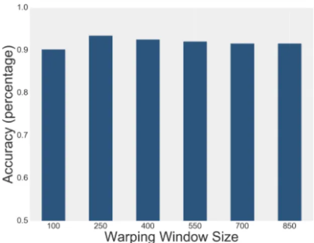
Fig. 8: Model comparison for position z with dif-ferent w values.

In order to find the best model, we have to find the best k and the best warping window size w. In our previous evaluation [14], it had been shown that a warping window size between 200 and 300 yields the best results. Therefore, we start by running the algorithm for different ks (1, 2, 3, 4 and 5) and a warping window w of 250. Figure 7 represents the accuracy results for positions x, y and z. The plots show that the algorithm achieves its best accuracy of 93%, when k is equal to 3, for a warping window of 250 for the z-axis position.

The next step is to use the best k and run the algorithm for different warping window sizes. Figure 8 presents the results of 6 new models that have been trained and tested for different ws of 100, 250, 400, 550, 700, 850, and k = 3. It is obvious that the algorithm has its best performance when the warping window size is 250.

Finally, when the optimal parameters have been found, the classifier, fitted with 90% training data, is being tested and evaluated against the 10% test data.

TABLE I: The final results for each parameter and position.

Feature Accuracy k Max Warping Window Comp. Time X 92.5% 2 250 ≈ 6 sec Y 88.5% 3 250 ≈ 6 sec Z 90.6% 3 250 ≈ 6 sec

Table I presents the final results of the classifier’s perfor-mance for each position x, y, z. The trained model achieves an accuracy of 92, 5% for position x, 88, 5% for position y and 90.6% for position z with the computational time of around 6 seconds for each 10 second long sliding time

window. In addition, the computation of each DTW distance for each time window can be easily parallelized, because each time window is relatively small and multiple windows can easily be loaded into memory.

Looking at the table II, which represents the results of the previous work, it is obviously seen that using a sliding window approach not only improved the accuracy, but also reduced the reduced the wait time to get the first prediction. TABLE II: The final results on the test data for each position [14].

Feature Accuracy k Max Warping Window Comp. Time X 90.7% 2 200 ≈ 45 sec Y 85.7% 3 200 ≈ 45 sec Z 88.6% 3 200 ≈ 45 sec

All presented results have been obtained by the proof of concept. The results prove that the kNN along with DTW not only can be used for offline time series classifications, but also can successfully classify streams of time series in a real time.

VI. CONCLUSION AND FUTURE WORK The main focus of this paper was to analyze a stream of flight data from a UAV following a pre-defined mission and predict the level of degradation of a body part, in this case of propellers, in real time. To achieve this goal, we have used k Nearest Neighbor as classification algorithm, along with Dynamic Time Warping as a distance measure for computing the similarity between two chunks of flights.

It is important to note that the presented results are improved than the ones in our previous work [14] and thus, demonstrates that the online mode using a sliding time window approach performs better, and speeds up the computation time. The reason is due to the fact that a single flight has been split into chunks, and each chunk has been individually labelled. This leads to an improved and more fine-grained definition of the level of degradation at the different stages of the mission. Essentially, instead of having one label, describing the entire flight, we have several labels, each describing a portion of the flight.

The advantage of this approach is that it can be applied to other experimental setups and can be used to estimate degradations, not only of propellers, but for any other body parts. Ideally, the flight data used for the prediction should be the one generated by the UAVs internal GPS sensors. Additionally, a model should only be trained for one type of degradation. In general, machine learning algorithm require a substantial amount of computing power. Running such al-gorithm onboard the UAV is feasible, but such computations do drain the battery much faster, effectively reducing the drone’s time to complete its mission. It is preferred to run the algorithm in the cloud and stream the flight data directly to the server.

Another possible extension for the current approach is to reduce the high computational cost of DTW distances using a

lower-bounding measure [24][25], which can reduce the cost of many tasks that rely on DTW. A lightweight algorithm would open the possibility of running the classifier directly on the drone without requiring a cloud solution.

A natural extension of this work consists in applying an unsupervised approach. This means that the degradations should be detected, without having prior knowledge of the possible problems. Such technique might discover many more degradations or anomalies than a supervised model. The proposed technique can be tailored for different scenar-ios and data.

As a future work, for the identification of degradation of an aircraft, the data collected by the internal GPS sensors of UAV will be used. This will give an advantage to run such technique on the aircrafts that perform outdoor missions. One usecase consists of monitoring a swarm of robots and detecting if there are any abnormal behaviors or if the formation has been broken.

It is also worth to mention that such solutions can be integrated into continuing airworthiness processes [26] of the aircrafts and system/component reliability and availability.

To conclude, it has been shown that the level of degrada-tion of a UAV can be predicted in an online mode, based on the analysis of flight coordinates. Both, autonomous robots and machine learning, are relatively new research areas and there are still many challenges ahead, especially in terms of high-performance online data mining and live identification of degradations and anomalies. Additionally, UAVs and other autonomous robots, have many more sensors that generate a huge amount of data. This data can be used and processed in many different and creative ways in order to discover new insight during autonomous or pre-defined tasks and allow for smarter and more advanced usage of robotic applications.

REFERENCES

[1] Kataria, Aman, and M. D. Singh. ”A Review of Data Classifica-tion Using K-Nearest Neighbour Algorithm.” InternaClassifica-tional Journal of Emerging Technology and Advanced Engineering 3.6 (2013): 354-360. [2] Lin Raz, Eliyahu Khalastchi, and Gal Kaminka. ”Detecting anomalies in unmanned vehicles using the mahalanobis distance.” Robotics and Automation (ICRA), 2010 IEEE International Conference on. [3] Stavrou, Demetris, et al. ”Fault detection for service mobile robots

using model-based method.” Autonomous Robots 40.2 (2016): 383-394.

[4] Plagemann, Christian, Cyrill Stachniss, and Wolfram Burgard. ”Ef-ficient failure detection for mobile robots using mixed-abstraction particle filters.” European Robotics Symposium 2006. Springer Berlin Heidelberg, 2006.

[5] Larrauri, Juan I., Gorka Sorrosal, and Mikel Gonzlez. ”Automatic system for overhead power line inspection using an Unmanned Aerial VehicleRELIFO project.” Unmanned Aircraft Systems (ICUAS), 2013 International Conference on. IEEE, 2013.

[6] Brotherton, Tom, and Ryan Mackey. ”Anomaly detector fusion pro-cessing for advanced military aircraft.” Aerospace Conference, 2001, IEEE Proceedings. Vol. 6. IEEE, 2001.

[7] Afridi, M. Jamal, Ahsan Javed Awan, and Javaid Iqbal. ”AWG-Detector: A machine learning tool for the accurate detection of Anomalies due to Wind Gusts (AWG) in the adaptive Altitude control unit of an Aerosonde unmanned Aerial Vehicle.” Intelligent Systems Design and Applications (ISDA), 2010 10th International Conference on. IEEE, 2010.

[8] Khalastchi, Eliahu, et al. ”Online anomaly detection in unmanned vehicles.” The 10th International Conference on Autonomous Agents and Multiagent Systems-Volume 1. International Foundation for Au-tonomous Agents and Multiagent Systems, 2011.

[9] Laurikkala, Jorma, et al. ”Informal identification of outliers in medical data.” Fifth International Workshop on Intelligent Data Analysis in Medicine and Pharmacology. Vol. 1. 2000.

[10] Pokrajac, Dragoljub, Aleksandar Lazarevic, and Longin Jan Latecki. ”Incremental local outlier detection for data streams.” Computational Intelligence and Data Mining, 2007. CIDM 2007. IEEE Symposium on. IEEE, 2007.

[11] Laxhammar, Rikard, and Gran Falkman. ”Online learning and sequen-tial anomaly detection in trajectories.” IEEE transactions on pattern analysis and machine intelligence 36.6 (2014): 1158-1173.

[12] Ahmad, Subutai, and Scott Purdy. ”Real-Time Anomaly Detection for Streaming Analytics.” arXiv preprint arXiv:1607.02480 (2016). [13] Lee, Yen-Hsien, et al. ”Nearest-neighbor-based approach to time-series

classification.” Decision Support Systems 53.1 (2012): 207-217. [14] Manukyan, Anush, et al. ”UAV degradation identification for pilot

notification using machine learning techniques.” Emerging Technolo-gies and Factory Automation (ETFA), 2016 IEEE 21st International Conference on. IEEE, 2016.

[15] Chaovalitwongse, Wanpracha Art, Ya-Ju Fan, and Rajesh C. Sachdeo. ”On the time series k-nearest neighbor classification of abnormal brain activity.” IEEE Transactions on Systems, Man, and Cybernetics-Part A: Systems and Humans 37.6 (2007): 1005-1016.

[16] Suguna, N., and K. Thanushkodi. ”An improved K-nearest neighbor classification using Genetic Algorithm.” International Journal of Com-puter Science Issues 7.2 (2010): 18-21.

[17] Park, Youngser, Carey E. Priebe, and Abdou Youssef. ”Anomaly detection in time series of graphs using fusion of graph invariants.” IEEE journal of selected topics in signal processing 7.1 (2013): 67-75. [18] Abid, Anam, Muhammad Tahir Khan, and C. W. de Silva. ”Fault detection in mobile robots using sensor fusion.”Computer Science & Education (ICCSE), 2015 10th International Conference on. IEEE, 2015.

[19] Duan, Zhuohua, Hui Ma, and Liang Yang. ”Fault detection for internal sensors of mobile robots based on support vector data description.” Control and Decision Conference (CCDC), 2015 27th Chinese. IEEE, 2015.

[20] Arrichiello, Filippo, Alessandro Marino, and Francesco Pierri. ”A de-centralized fault detection and isolation strategy for networked robots.” Advanced Robotics (ICAR), 2013 16th International Conference on. IEEE, 2013.

[21] Wu, Xindong, et al. ”Top 10 algorithms in data mining.” Knowledge and Information Systems 14.1 (2008): 1-37.

[22] iRobot Roomba

https://www.irobot.com/For-the-Home/Vacuuming/ Roomba.aspx

[23] Video of the UAV Good and Worst flight

https://www.dropbox.com/s/tfc6jjvrzqy5l2d/UAV_ Good_Worst_Flight.mp4?dl=0

[24] Yang, Peng, et al. ”A tighter lower bound estimate for dynamic time warping.” Acoustics, Speech and Signal Processing (ICASSP), 2013 IEEE International Conference on. IEEE, 2013. APA

[25] Rakthanmanon, Thanawin, et al. ”Searching and mining trillions of time series subsequences under dynamic time warping.” Proceedings of the 18th ACM SIGKDD international conference on Knowledge discovery and data mining. ACM, 2012.

[26] Correia, Vitor Monteiro. ”The Aircraft Maintenance Program and its importance on Continuing Airworthiness Management.”