Direction des bibliothèques
AVIS
Ce document a été numérisé par la Division de la gestion des documents et des archives de l’Université de Montréal.
L’auteur a autorisé l’Université de Montréal à reproduire et diffuser, en totalité ou en partie, par quelque moyen que ce soit et sur quelque support que ce soit, et exclusivement à des fins non lucratives d’enseignement et de recherche, des copies de ce mémoire ou de cette thèse.
L’auteur et les coauteurs le cas échéant conservent la propriété du droit d’auteur et des droits moraux qui protègent ce document. Ni la thèse ou le mémoire, ni des extraits substantiels de ce document, ne doivent être imprimés ou autrement reproduits sans l’autorisation de l’auteur.
Afin de se conformer à la Loi canadienne sur la protection des renseignements personnels, quelques formulaires secondaires, coordonnées ou signatures intégrées au texte ont pu être enlevés de ce document. Bien que cela ait pu affecter la pagination, il n’y a aucun contenu manquant.
NOTICE
This document was digitized by the Records Management & Archives Division of Université de Montréal.
The author of this thesis or dissertation has granted a nonexclusive license allowing Université de Montréal to reproduce and publish the document, in part or in whole, and in any format, solely for noncommercial educational and research purposes.
The author and co-authors if applicable retain copyright ownership and moral rights in this document. Neither the whole thesis or dissertation, nor substantial extracts from it, may be printed or otherwise reproduced without the author’s permission.
In compliance with the Canadian Privacy Act some supporting forms, contact information or signatures may have been removed from the document. While this may affect the document page count, it does not represent any loss of content from the document.
Université de Montréal
Analyse spatiale en écologie: développenlents méthodologiques
par
Guillaume Blanchet
Département de Sciences Biologiques Faculté des Arts et des Sciences
Mémoire présenté à la Faculté des Études Supérieures en vu de l'obtention du grade de
Maître ès science (M.Sc.)
Août 2007
Identification du Jury
Université de Montréal Faculté des Études Supérieures
Ce mémoire intitulé:
Analyse spatiale en écologie: développements méthodologiques
présenté par Guillaume Blanchet
a été évalué par un jury composé des personnes suivantes:
François-Joseph Lapointe ... Président-rapporteur
Pierre Legendre ... Directeur·de recherche.
Daniel Boisclair ... Membre du jury
11
RÉSUMÉ
Ce travail, à deux volets, propose d'une part [1] l'amélioration d'une méthode de sélection de variables afin qu'elle soit mieux adaptée à des variables spatiales orthogonales et, d'autre part, [2] les cartes de vecteurs propres asymétriques qui constituent une nouvelle méthode permettant de générer des variables spatiales en considérant l'asymétrie spatiale d'un processus écologique.
[1] La méthode progressive de la régression pas à pas est souvent utilisée en écologie pour sélectionner unjeu réduit de variables explicatives. C'est une méthode efficace pour construire un modèle statistique concis. Par contre, son utilisation avec des variables spatiales construites dans le cadre des cartes de vecteurs propres de Moran (ou
Moran 's eigenvector maps, MEM) a tendance à surestimer la quantité de variances
expliquée et à gonfler l'erreur de type 1. Le premier chapitre de ce travail propose une innovation à cette méthode de sélection pour pallier à ces problèmes. Une procédure en deux étapes est développée. En premier lieu, un test global en utilisant tout le jeu de variables spatiales doit être réalisé. Si, et seulement si, le test global est significatif, la méthode progressive de la régression pas à pas peut être appliquée. Pour éviter la surestimation de la variance expliquée, la régression pas à pas doit être faite en utilisant deux critères d'arrêt, soit (1) le critère de réjection alpha, ce qui est commun pour tout type de régression pas à pas, et (2) le coefficient de détermination multiple ajusté (R2 a) calculé
avec toutes les variables spatiales disponibles. Lorsqu'une variable spatiale fait dépasser le seuil fixé pour l'un ou l'autre des deux critères, cette variable est rejetée et la sélection s'arrête.
[2] La répartition spatiale des espèces, tant animales que végétales, terrestres qu'aquatiques, est influencée par de nombreux facteurs, comme les gradients physiques et biogéographiques. Par exemple, la direction du vent dominant ou d'un courant induit des gradients qui peuvent influencer la répartition spatiale de nombre d'espèces alors que des événements historiques (e.g. une glaciation) peuvent créer des gradients biogéographiques.
iii
l'asymétrie d'un processus contrôlant lorsqu'une étude de la répartition spatiale est faite le long d'un gradient. Le deuxième chapitre de ce travail présentera une nouvelle méthode modélisant la répartition des espèces dans l'espace en présence d'un processus asymétrique connu. Cette méthode est une extension des MEM. La méthode produit les cartes de . vecteurs propres asymétriques (ou asymmetric eigenvector maps, AEM).
Chacun des chapitres de ce travail sera illustré par des données écologiques réelles. Le premier chapitre est illustré par l'analyse de données du Parc national Bryce Canyon (Utah, États-Unis d'Amérique) alors que le second est illustré par l'analyse de données de contenus stomacaux d'ombles de fontaine (Salvelinusfontinalis) provenant de 42 lacs de la
réserve Mastigouche, Québec, Canada.
Mots-clés: méthode progressive de la régression pas à pas, asymétrie spatiale, coordonnées principales de matrice de voisinage (PCNM), carte de vecteurs propres de Moran (MEM), carte de vecteurs propres asymétriques (AEM), réserve Mastigouche, Salvelinus fontinalis,
SUMMARY
This two-chapter work presents first an improvement of the forward selection procedure that is better suited for orthogonal spatial variables. It also proposes a new method to generate spatial variables, which considers the spatial asymmetry of an ecological process. These variables are called asymmetric eigenvector maps.
iv
The first chapter of this work proposes a new way of using forward selection that is weU adapted to eigenfunction-based spatial filtering methods. The classical forward selection procedure carried out on orthogonal spatial variables presents a highly inflated rate of type l error. To prevent this, we propose a two-step procedure. First, a global test using aIl spatial variables must be carried out. If, and only if, the global test is significant, one can proceed with forward selection. Furthermore, to prevent overesimation of the explained variance, the forward selection has to be carried out with two stopping criteria:
(1) the usual alpha level of rejection and (2) the adjusted coefficient of multiple
determination (R2a) calculated with aU spatial variables. When forward selection identifies a variable that brings one or the other criterion over the fixed threshold, this variable is
rejected and the procedure stops.
Distributions of species, animaIs or plants, terrestrial or aquatic, are influenced by numerous factors such as physical and biogeographical gradients. Dominant wind and CUITent directions cause the appearance of gradients in physical conditions whereas biogeographical gradients can be the result ofhistorical events (e.g. glaciations); such factors are known to influence the spatial distributions of many species. No spatial modelling technique has been developed to this day that considers the asymmetry of the controlling factors when studying species distributions along a gradient. Here will be presented a new spatial modelling method that can model species spatial distributions generated by a known asymmetric process. This method is an eigenfunction-based spatial filtering method; it pertains to the same general framework as Moran's eigenvector maps (MEM) analysis. The new method is called asymmetric eigenvector maps (AEM). To
v
illustrate how this new method works, AEM are compare to MEM through simulations and with an ecological example where a known asymmetric forcing is present.
An ecological illustration is presented for each chapter. The frrst chapter uses plant data gathered in Bryce Canyon National Park (Utah, USA). The second chapter uses dietary habits of brook trout (Salvelinus fontinalis) sampled in 42 lakes in the Mastigouche
Reserve, Québec.
Key words: Forward selection, spatial asymmetry, principal coordinates ofneighbor
matrices (PCNM), Moran's eigenvector maps (MEM), asymmetric eigenvector maps (AEM), Mastigouche Reserve, Salvelinus fontinalis, Bryce Canyon National Park.
VI
TABLE DES MATIÈRES
RÉSUMÉ ... ii
SUMMARY ... : ... iv
TABLE DES MATIÈRES ... vit LISTE DES TABLEAUX ... vii
LISTE DES FIGURES ... ' ... viii
REMERCIEMENTS ... xii
INTRODUCTION ... 1
CHAPITRE 1 : F orward selection of explanatory spatial variables ... 8
Abstract ... 10
Introduction ... 10
Difference between PCNM and MEM variables ... Il Forward selection: a huge type 1 error ... 12
Global Test: a way to achieve a correct type 1 error rate ... 14
Structured Response Variables: towards an accurate modeling ... 15
Exrunple: Bryce Canyon Data ... 19
Discussion ... 20
CHAPITRE 2 : Modelling spatial asymmetry in ecological data ... 33
Abstract ... 34 Introduction ... 35 Method ... 36 Simulation study ... 39 Ecological illustration ... 44 Discussion ... 48 CONCLUSION ... 66 BIBLIOGRAPHIE ... 67
VII
LISTE DES TABLEAUX
CHAPITRE 1
Table 1: Percentage oftime when aU the variables used to create the response variable, and only those, were chosen by the forward selection procedure.
CHAPITRE 2
Table 1: Weighting function and a parameter giving the highest explained variance when modeling each structure of each set of simulation, with AEM or MEM. Results were obtained after 1000 simulations done with each combination of weighting function (2) and a parameter (10). The same response variables were used to compare AEM and MEM variables.
Table 2: Comparison of spatial models of brook trout di et obtained from 7 different modeling methods. While Magnan et al. (1994) used a subset of37lakes and a cutoff level of a 0.10 in their forward selection in CCA, we used the full set of 42 lacs and a cutoff level of a = 0.05 for the results presented in this table.
viii
LISTE DES FIGURES INTRODUCTION
Figure 1 : Principe de l'analyse spatiale PCNM, basée sur les coordonnées principales d'une matrice de voisinage (matrice tronquée de distances euclidiennes entre les sites). (Modifié de Legendre et Borcard 2006).
Figure 2 : Principe de l'analyse spatiale MEM.
CHAPITRE 1
Figure 1 : Result of 5000 simulations of forward selection when only alpha is used as a stopping criterion. The response variable is random normal. (a) R2a for each simulation, black = BEM, grey = PCNM. The mean of the 5000 simulations is
presented with a line going through the distribution. (b) Number of PCNMs selected by forward selection. (c) Number ofBEMs selected by forward selection.
Figure 2 : Type l error of BEMs on series of 100 data points randomly selected from four distributions. For each distribution, 5000 independent simulation were
completed. The error bars represent 95% confidence intervals.
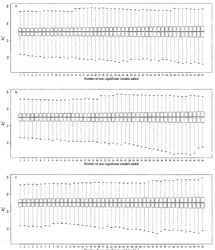
Figure 3 : Variation of R2 a when randomly selected spatial variables are added to a model
already containing the correct explanatory variables. ~patial variables were added one at a time until none was left to add. 5000 simulations were done. Whiskers: extreme values. (a) Results for PCNMs. (b) Results for positively autocorrelated BEMs. (c) Results for negatively autocorrelated BEMs.
IX
Figure 4 : Comparison of a forward selection done on PCNMs with both the R2 a and alpha level as stopping criteria (a-b, e-f, i-j) with one where only the alpha criterion (c-d, g-h, k-l) was used. Three different situations are presented: (1) the standard deviation of the deterministic part of the response variable is the same as the standard deviation ofthe error (a-d), (2) the standard deviation of the error is 0.25 times that of the standard deviation of the deterministic part (e-h) and (3) the standard deviation of the error is 0.001 times that of the standard deviation of the deterministic part (i-l). The left-hand side presents the correct selections made by the forward selection, i.e., the variables selected were the ones used to create the response variable. The right-hand side shows the bad selections, i.e. the variables selected were not the ones used to create the response variable. 5000 simulations were mn for each magnitude of error.
x
CHAPITRE 2
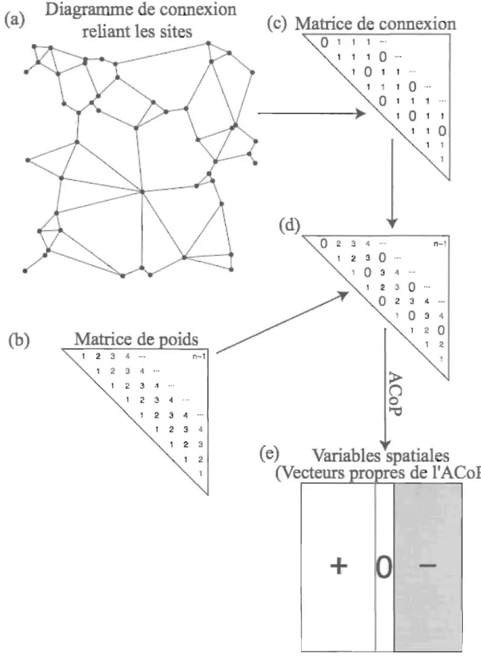
Figure 1: Schematic representation of AEM analysis using a fictive example. Sites are linked together with a connection diagram (a-b), which in turn will be used to construct a sites by link matrix (c). Weights can be added to the links (column) of this matrix. Descriptors (AEM variables) are than constructed through the
calculation of SVD or PCA eigenvectors (d). Construction of AEM variables can also be done through the calculation of a distance matrix and the calculation of eigenvectors via PCoA.
Figure 2: Type 1 error of AEM analysis (b, d) with connection diagram and points (a) and (c) respectively. No weights were used in (a), whereas the inverse of the distance was used as weight in (c). The large arrows present the direction of the
asymmetry considered for (a) and (c). Response variables were randomly selected for each point from four different distributions. Each run consisted of 5000 independent simulations. The errors bars in (b) and (d) represent 95% confidence intervals.
Figure 3: (a) Connection diagram used to create AEM and MEM variables. Arrows represent direction of influence of each site on others; the se directions were considered to construct AEM variables but not for MEM variables. (b) Eight basic structures (SI to S8) used to generate response variables. Numbers are weights added, prior to adding random normal noise, to one whole line (1 to 10) of the regular grid used (a) for simulations. Each pair of structure presents a symmetric (even numbered structure) and an asymmetric (odd numbered structure) pattern in the generation of the data.
Xl
Figure 4: Variance explained (R2a) for the best set of AEM (fullline) and MEM (dotted line) variables for each of the 8 structures presented in Figure 3. (a-c) present results of univariates simulations where the error parameter was randomly chosen from a normal distribution with a standard deviation of 1, 2, and 3 respectively. (d) presents results of multivariates simulations where the error parameter was randomly chosen from a normal distribution with a standard deviation selected from a uniform distribution with a minimum of 1 and a maximum of 3. Error bars represent 95% confident intervals. Each run consists of 1000 independent simulations. Lines linking error bars were plotted to prevent confusion between results of AEM and MEM analysis.
Figure 5: Schematic map of the river network in the Mastigouche Reserve. Lakes are numbered L-l to L-43; there is no lake L-20. Edges are numbered e-l to e-65. Adapted from Magnan et al. (1994).
Figure 6: RDA triplot (axes 1 and 2) showing the 42 lakes (open square), 9 prey categories (5 are shown by arrows, the other 4 were very short and contributed little to the ordination plane), and 13 AEM variables (lines). Axes 1 and 2 were the only significant axes.
Figure
?:
Bubble plot maps of the RDA fitted site scores for (a) axis 1 and (b) axis 2; black bubbles are positive, white bubbles are negative; circ1e sizes are proportional to the absolute values represented. (c) Four groups K-means partition of the lakes plotted on the river network map.XII
REME RCIEMENTS .
En premier lieu, je souhaite remercier mon directeur de recherche, Pierre Legendre. Il aurait été impossible pour moi de faire ce projet sans son support intellectuel et financier. Son enthousiasme contagieux pour la recherche, la bonne bouffe, le bon vin, les Macs ... et tant d'autres choses n'ont fait que rendre l'expérience plus mémorable. Le dynamisme du Labo Legendre a été pour moi un environnement de croissance intellectuelle fantastique sur tous les plans (de l'histoire à la statistique bayesienne en passant par les recettes de homard au chocolat). Pierre a été pour moi plus qu'un mentor, il a aussi été un ami qui m'a ouvert les yeux sur le monde.
Très près derrière, je désire aussi remercier Daniel Borcard pour tout le support qu'il m'a accordé autant pour mes travaux de recherche que pour l'enseignement de la biostatistique. Son esprit un peu tordu pour régler des problèmes de tout ordre ainsi que les discussions élaborées sur de si nombreux sujets m'ont permis d'évoluer dans mon
cheminément personnel.
Aussi, j'aimerais remercier les membres du Labo Legendre qui furent présents lors de mon séjour: Marie-Hélène Ouellette, Sébastien Durand, Pedro R. Peres-Neto, Stéphane Dray, Einar Heegaard, Elaine Hooper, Miquel DeCacères Ainsa, Philippe Casgrain et Charleyne Bachraty; vous m'avez fait voir de nombreuses facettes de la recherche
scientifique en rendant le sujet abordable pour moi ... qui étais fraîchement sorti du monde de la physiologie animale.
Ensuite, je voudrais rendre un hommage posthume aux quelques virus de la grippe qui ont réussi à m'affecter pendant ces deux dernières années. Malgré les périodes de faiblesse qu'ils m'ont apportées, ces derniers m'ont obligé à prendre quelques jours de repos qui ont été plus qu'appréciés.
Pour terminer, je dédie ce mémoire à mes parents Richard et Diane. Leur support moral, les moments de détente qu'ils m'ont imposés et les valeurs qu'ils m'ont transmises ont rendu l'achèvement de ce travail possible.
INTRODUCTION
L'importance de l'hétérogénéité spatiale en écologie est bien connue et ce depuis longtemps (Kolasa et Rollo 1991). Par contre, les méthodes permettant d'étudier ces phénomènes sont arrivées beaucoup plus tardivement. En 1989, Legendre et Fortin ont publié un article qui s'avéra être un point tournant pour l'analyse spatiale en écologie. Ils présentèrent plusieurs méthodes provenant de domaines extérieurs à l'écologie permettant d'expliquer l'impact des phénomènes spatiaux sur la répartition des communautés
végétales. Ces méthodes ont été utilisées dans d'autres sphères de l'écologie comme la limnologie (e.g. Cooper et al. 1997), l'océanographie (e.g. Planque et al. 1997), l'écologie animale (e.g. Bergin 1992).
Ensuite, plusieurs écologistes plus versés dans la statistique et les mathématiques se sont lancés dans le développement de méthodes pour analyser spécifiquement l'espace en écologie. Un bon exemple de développement méthodologique fait par un écologiste pour mieux comprendre les phénomènes spatiaux en écologie est la partition de la variation (Borcard et al. 1992). Cette méthode a été développée originalement pour mieux comprendre quelle portion de la variance expliquée est uniquement due aux variables spatiales d'un modèle, uniquement aux variables environnementales, ainsi qu'à une combinaison de ces deux groupes de variables.
Avec la partition de la variation, il devenait impératif de trouver une façon de générer des variables permettant de bien modéliser la répartition spatiale des organismes. La méthode la plus simple permettant de générer ce genre de variables, connue à l'époque du développement de la partition de la variation, était de calculer un polynôme de deuxième ou de troisième ordre à partir des coordonnées géographiques (Legendre 1990). Ceci
consiste à prendre les cordonnées XY des sites et les élever au premier (X et Y), au
deuxième (X, Y, XY, X2 et y2) ou au troisième degré (X, Y, XY, X2, y2, X2y, Xy2, X3 et
y3). Ce polynôme formait le tableau des variables explicatives dans une régression ou une analyse canonique. Il devenait donc possible d'analyser des structures spatiales dans un contexte écologique. Ce type de méthode a par contre un défaut: pour pouvoir modéliser la
2
distribution d'organismes à une échelle relativement fine, il est nécessaire de disposer d'un polynôme extrêmement long. Quoique mathématiquement possible, l'utilisation d'un polynôme d'ordre supérieur à trois présente plusieurs problèmes. La robustesse d'un test statistique peut être diminuée si trop de variables sont incorporées dans un modèle. Ce problème est particulièrement important lorsque le nombre d'observations est faible, ce qui est fréquemment le cas en écologie. Un autre problème lié à l'utilisation d'un polynôme de grand ordre (plus que trois) est la difficulté qu'on peut avoir à interpréter l'effet de ces variables sur le tableau-réponse.
Pour pallier aux inconvénients qu'engendre l'utilisation des polynômes des coordonnées géographiques, Borcard et Legendre (2002) ont développé les coordonnées principales de matrices de voisinage (Principale coordinate of neighbour matrices, PCNM, en anglais); l'acronyme anglais sera utilisé dans le reste du texte pour éviter toute confusion avec l'acronyme français des cartes de vecteurs de Moran. Les PCNM sont des variables orthogonales issues d'une décomposition spectrale d'une matrice de distances tronquée calculée à partir des coordonnées géographiques des sites d'échantillonnage (Figure 1). Une matrice de distance tronquée consiste en une matrice de distance où toutes les distances plus grandes que la plus grande distance dans la chaîne permettant de relier tous les sites ensemble sont remplacées par une valeur très grande (4 fois la plus grande distance considérée, ou plus). Elles ont l'avantage de permettre de déceler des variations à échelle fine et ce même si un nombre très restreint de sites ont été échantillonnés. Elles peuvent être utilisées dans des contextes très variés. Borcard et al. (2004) présentent plusieurs situations écologiques très différentes où l'analyse PCNM a produit des résultats très intéressants.
Il a ensuite été montré par Dray et al. (2006) que les PCNMs font partie d'un cadre général, les cartes de vecteurs propres de Moran (Moran 's eigenvector maps, MEM en anglais); l'acronyme anglais sera utilisé dans le reste du texte pour éviter toute confusion avec celui des coordonnées principales de matrices de voisinage. Alors que les PCNM sont uniquement basées sur les distances entre les sites échantillonnés, le cadre des MEM
3
présente une façon de créer des variables où non seulement les distances entre les sites peuvent être prises en considération, mais aussi le nombre de voisins; les sites peuvent êtres reliés entre eux par un diagramme de connexions permettant de définir quels sites ont une influence les uns sur les autres. La figure 2 présente schématiquement la construction de variables spatiales construites dans le cadre des MEM. Les MEMs permettent une très grande flexibilité qu'aucune autre méthode d'analyse spatiale n'avait jusqu'alors.
Les PCNMs, comme les MEMs, ont aussi leurs défauts et leurs limites. Ces deux méthodes permettent de générer un nombre très important de variables spatiales. Pour les PCNMs, il est fréquent de voir 2n/3 variables générées, n étant le nombre de sites
échantillonnés. Pour les MEMs, il arrive souvent qu'il y ait (n - 1) variables générées, ce qui est encore pire, puisque avec autant de variables, un test statistique est impossible à faire par manque de degrés de liberté.
Ces deux méthodes se veulent généralistes: elles peuvent être utilisées dans toutes les situations où l'on souhaite modéliser la structure spatiale des données échantillonnées. Malheureusement, certaines situations requièrent des méthodes plus spécifiques. Les PCNMs et les MEMs tentent de modéliser la répartition spatiale d'organismes sans prendre en considération des connaissances qu'on pourrait posséder a priori sur un milieu étudié.
Par exemple, si on tente de modéliser la répartition spatiale d'organismes dans une rivière à l'aide des PCNMs ou des MEMs, même si ces dernières sont très flexibles, aucune de ces méthodes ne permet de prendre en considération le fait qu'un courant puisse influencer de façon directionnelle la répartition spatiale des organismes étudiés.
Dans toutes ces méthodes de modélisation spatiale, un grand nombre de fonctions sont générées pour décrire les relations spatiales entre les sites d'échantillonnage. Il est intéressant dans certains cas de réduire le nombre de variables spatiales explicatives des données écologiques à l'aide d'une des méthodes dé sélection menant à un modèle parcimonieux. Un modèle parcimonieux a plus de pouvoir prédictif (Gauch 1993,2003). Cela est désirable par exemple lors de la formulation de sous-modèles spatiaux
4
variables spatiales dans un diagramme d'ordination. La méthode couramment employée en analyse canonique est,la sélection ascendante (jorward selection, en anglais) des variables
explicatives. Or on sait que cette méthode e,st trop libérale; en d'autres termes, elle a
tendance à incorporer dans le modèle des variables qui n'ont qu'un effet aléatoire au niveau de la population statistique. Parce que nous analysons un échantillon de taille réduite, ces variables peuvent, par hasard, modéliser une partie du bruit qui se trouve dans les données.
Les deux chapitres de ce travail ont pour but de résoudre les deux problèmes mentionnés ci-dessus.
Le premier chapitre propose une nouvelle méthode de sélection de variables
spatiales orthogonales. Il a pour but d'avertir les utilisateurs de cette méthode à propos des comportements capricieux de la sélection progressive lorsque cette dernière est utilisée pour sélectionner des variables spatiales orthogonales. Ce chapitre propose aussi une nouvelle procédure de sélection progressive pour sélectionner des variables provenant du cadre des MEM où le nombre de variables spatiales explicatives est (n - 1).
Cette nouvelle procédure sera validée à l'aide de simulations. Un jeu de données sur la biodiversité des plantes vasculaires du Parc national de Bryce Canyon (Utah, États-Unis d'Amérique) sera utilisé pour illustrer comment cette nouvelle procédure réagit dans une situation écologique réelle.
Le second chapitre de ce travail présente une nouvelle méthode pour générer des variables spatiales. Il est bien connu que la répartition spatiale des espèces peut être influencée par un ou des gradients des variables environnementales (Huston 1996). Beaucoup de gradients sont induits par des processus spatiaux asymétriques. Malgré les développements méthodologiques importants qui ont permis de mieux comprendre
comment les structures spatiales influencent la répartition des espèces, aucune méthode ne considère les processus asymétriques. La méthode développée ici entre dans le cadre des méthodes de filtrage spatial basées sur le calcul de valeurs et de vecteurs propres, concept développé par Griffith et Peres-Neto (2006).
5
À échelle fine comme large, la répartition spatiale des espèces est souvent structurée selon un ou plusieurs gradients, biotiques et/ou abiotiques. Nous proposons d'utiliser des variables spatiales qUI sont asymétriques par construction pour étudier la répartition spatiale de communautés d'espèces qui sont influencées par des gradients. Dray et al. (2006)
déplorent l'absence de méthode considérant l'asymétrie spatiale; notre article servira à combler cette lacune dans la littérature. Comme pour les MEMs, les variables asymétriques présentées dans ce chapitre proviennent d'un cadre général très flexible permettant de générer des variables spatiales asymétriques. Les variables créées dans ce cadre s'appellent des cartes de vecteurs propres asymétriques (asymmetric eigenvector maps, AEM, en anglais); l'acronyme anglais sera utilisé ici. Ces variables se veulent appropriées pour des situations où les processus environnementaux influençant les organismes étudiés possèdent une asymétrie spatiale connue (e.g. dans une rivière, un fleuve ou un courant marin). Ce nouveau développement sera validé par des simulations créées dans un contexte
bidimensionnel. Un jeu de données sur les contenus stomacaux des ombles de fontaine
(Salvelinus fontinalis) dans 42 lacs de la réserve Mastigouche sera utilisé pour illustrer
l'utilisation des AEMs dans une étude écologique réelle. Une comparaison entre les AEMs et plusieurs autres méthodes, dont les MEMs et les PCNMs, sera faite pour ce même jeu de données.
Donnœ.s
Variable
hiSd:
,....-_ _ _ _ _ _ _
Ob_~ée
.
~ , 1 l 2 :l 4 :S 6 i 8, 9 10 H X 6/
(coorOOM~~~::::mnc~ euclidienn~
Distances euclidiennes
tronquée =matriœ de voisinage
4 :S "0 oo.lt-J .3 4 .5 0.0 S 0.0 12.34:5'00 l 2:3 :5 ... .5 4
Régression multiple
ou analyse canonique
y
X(+)
Figure 1Vecteurs propres
poss'édant une·
valeur propre positive
=
variables spatiales PCNM
Analyse en
coordonnées principales
+
(a)
(h)
•
Diagramme de connexion
reliant les
sites
1 2 l ,~ .. - n-1 r 2 3 " , .. Figure 2 :1 <1. -2: 3 4 .. , , 2 :! ,~
(c) Matrice
de
connexion
o
1 1 1 ... 1 1 10
10
~ t ... l0
..
1 1o
(d)~
_ _ _
--.
2 3 -1 ... n-' , 2 :10
...
10
:)
4 1 2 3 0 ...o
2 .~ ...;>
n
o
"'do
:)
.,
! 20
7( e)
Variables spatial
e
s
(Vecteurs propres de l'ACoP)
+
0
-
11
,
Chapitre 1
9
Statistical Report Submitted to Ecology
F
orward selection of explanatory spatial variables.
F. GUILLAUME BLANCHET!,2, PIERRE LEGENDRE!, AND DANIEL BORCARD!
! Département de sciences biologiques, Université de Montréal, C.P. 6128, succursale Centre-ville, Montréal, Québec, Canada H3C 317
2 Corresponding address: F. Guillaume Blanchet, Départment de sciences biologiques, Université de Montréal, c.P. 6128, succursale Centre-ville, Montréal, Québec, Canada H3C 317. E-mail:
10
Abstract. This report proposes a new way ofusing forward selection that is well
adapted to eigenbased spatial filtering methods. The classical forward selection carried out on orthogonal spatial variables presents a very inflated type 1 error. To prevent this, we propose a two steps procedure. First, a global test using all spatial variables must be carried out. If, and only if, the global test is significant, one can proceed with a forward selection. Furthermore, to prevent overesimation of the explained variance, the forward selection has to be carried out with two stopping criteria (1) the usual alpha level of rejection and (2) the adjusted coefficient of multiple determination (R2 a) calculated with all spatial variables. When forward selection identifies a variable that brings one or the other criterion over the fixed threshold this variable is rejected and the procedure is stopped. This new technique is validated with simulations and an ecological example is presented with data from Bryce Canyon National Park (Utah, USA).
Key words: Principal coordinates ofneighbor matrices (PCNM), Moran's eigenvector
maps (MEM), spatial analysis, simulations, type 1 error
INTRODUCTION
Since the introduction of principal coordinates of neighbor matrices (PCNM)
(Borcard and Legendre 2002, Borcard et al. 2004) and of Moran's eigenvector maps (MEM) (Dray et al. 2006), ecologist have been faced with the problem of having to handle large numbers of spatial explanatory variables in their analyses. In their conc1uding remarks, Bellier et al. (2007) st~ted: "PCNM requires methods to choose objectively the composition, number, and form of spatial submodels". We propose a new method for selecting spatial submodels for those types of variables. The new method is completely independent of the user's knowledge of the data under study.
An automatic selection procedure is used in most cases to select a subset of explanatory variables objectively. Having fewer variables that explain almost the same amount of variance is interesting; it retains enough degrees of freedom for testing the
F-Il
statistic in situations where the number of observations is smaH because observations are very costly. Furthermore, a parsimonious model has greater predictive power (Gauch 1993, 2003). One method very often used for selecting variables in ecology is forward selection. It presents the great advantage of working even when the initial dataset has more explanatory variables then sites, which is often the case in ecology. Since forward selection is being used more and more to select spatial variables (e.g. Borcard et al. 2004, Brind'Amour et al. 2005, Duque et al. 2005, Telford and Birks 2005, Halpern and Cottenie 2007), it is this report's goal to warn researchers against the sometimes capricious behavior offorward selection when selecting orthogonal spatial variables. We also propose a new forward selection procedure to select variables constructed through an eigenfunction-based spatial filtering method where the number of spatial explanatory variables is equal to (n - 1), where
n is the number of objects.
The procedure will be presented and validated with the help of simulated data. To illustrate how it reacts on real ecological data, we shaH use the Bryce Canyon National Park (Utah, USA) dataset.
DIFFERENCE BETWEEN PCNM AND MEM VARIABLES
ME Ms are a general framework to construct the many variants of orthogonal,
eigenvector-based spatial variables like PCNMs and distance-based eigenvector maps (Dray et al. 2006). For example, PCNMs are constructed on the basis of a distance criterion. This is not necessarily the case of other MEMs that can be constructed based on a connection diagram, a number of neighbors, etc. Detailed explanation of the construction of PCNMs and MEMs are presented in Borcard and Legendre (2002) and Dray et al. (2006)
respectively.
In this report, we will use two types of spatial variables out of the MEM framework to present our new approach of forward selection and investigate its properties by numerical simulations. The first type is PCNMs because they are the most widely used at the moment
12
in ecology (e.g. Duque et al. 2005, Kohler et al. 2006). PCNM is an eigen-based spatial decomposition method that creates spatial variables (PCNM eigenfunctions) through a truncated distance matrix initiaIly constructed from the geographical coordinates of the study sites. The other type is the simplest construction from the MEM framework, which we caU binary eigenvector maps (BEM) in this report. BEM are constructed from a connexion diagram, which, in the particular case of a transect, links aIl sites from left to right. No weights will be added to the links in the simulations presented in this paper. The connexion matrix derived from the connexion diagram is used directly to build spatial variables through a principal coordinate analysis (PCoA). AlI simulations and analyses were carried out on an irregular transect of 100 sites. For irregularly spaced sites, PCNMs and BEMs represent two extreme types in the MEM framework (Dray et al. 2006).
FORW ARD SELECTION: A HUGE TYPE l ERROR
The simulations presented below show that, when used in the traditional manner (i.e., step-by-step introduction of explanatory variables with a test of the partial contribution of each variable to be entered), forward selection of orthogonal spatial variables presents two problems: (1) an inflated type l error, and (2) an overestimation of the amount of variance explained. In a first set of simulations to measure the type l error rate, we created a random normal response variable along a transect containing 100 irregularly spaced
simulated sampling sites. The site positions along the transect were created using a random uniform generator. The same transect was used for aIl simulations. The simulations differ in the data generated at those specific sites. PCNMs were computed from the spatial
coordinates of the points along the transect, and a forward selection was carried out to identify the PCNM variables best suited to model the response variable, with a stopping a
level of 0.05. To increase computation speed, we ran aIl analyses using a parametric
forward selection procedure, adequate here because the simulated data were random normal. Parametric tests should not, however, be used with non-normal data such as tables of
13
species abundances. In such cases, randomization procedures should be used (Pitman, 1937a, 1937b and 1938). We repeated this procedure with 5000 independent sets ofrandom normal data. The same simulations were repeated with BEMs.
The simulation results are presented in Fig. 1. On PCNMs the procedure behaved correctly roughly 6% of the time only, selecting no PCNM to model a random variable, i.e., the overall type 1 error rate was about 94%. This is astonishingly high when compared to the expected rate of 5%. Very often in the simulations (about 73% of the cases), one to four PCNMs were selected to model random noise. Sometimes, up to 14 PCNMs were admitted into the model. These results show that forward selection yields a hugely inflated type 1 error. When forward selection was applied to BEMs, results were even more alarming. Only once in 5000 tries did the forward selèction lead to the correct result of not selecting any BEM. Almost 60% of the time, 7 to 17 BEM variables were selected incorrectly. As was the case for PCNM variables, very large numbers of BE Ms were sometimes selected (up to 62). These results show that one cannot run a forward selection without sorne form of
preliminary, overall test. They prompted us to find new criteria to improve the type 1 error of forward selection. This meant (1) to devise a rule to decide when it is appropriate to run a forward selection, and (2) to strengthen the stopping criterion of the forward selection to prevent it from being overly liberal.
Using numerical simulations, Ohtani (2000) has shown that the Ezekiel (1930) adjusted coefficient of multiple detennination (R2 a) is an unbiased estimator of the real contribution of a set of explanatory variables to the explanationof a response variable. Had the simulations presented above given accurate results, the adjusted coefficient of multiple deterrnination would have been zero or close to zero aU the time. In our results, after 5000 simulations, the mean of the R2a statistics is 13.2 % for PCNM and 47.2 % for BEM. Why do the R2 a values diverge so strongly from zero? The fundamental problem lies with the
forward selection procedure, which is exacerbated by the nature of these spatial variables. PCNM and BEM variables are structured in such a way that they are more suited than other types of variables to fit noise in the response data. The number of PCNM variables is at
most 2n!3 whereas the number ofBEM variables is (n 1). Besides being numerous, these variables are also orthogonal to one another, whieh means that each variable ean model entirely different aspects of a response variable. Fig. 1 b shows the number of PCNM variables selected during the 5000 simulations above, and Fig. le shows corresponding results for BEM variables. These graphs show that more BEM variables than PCNMs are incorrectly sel~cted, simply because they are more numerous. Thioulouse et al. (1995) suggest that eigenvectors associated to small positive or negative eigenvalues are only weakly spatially autocorrelated. With that in mind, we could expect the variance in our unstructured response variables to be "explained" mainly by PCNM and BEM variables With small eigenvalues. This was not the case: results show that all eigenvectors were selected in roughly the same proportions (see Appendix A for details).
GLOBAL TEST: A W A y TO ACHlEVE A CORRECT TYPE 1 ERROR RATE
14
To prevent the inflation of type 1 error (our first goal), a global test needs to be done prior to forward selection. This is the first important message of this report. A global test means that aIl orthogonal variables created in the PCNM or BEM procedure are used together to model the response variable. However, with BEMs, there are often n 1 spatial variables created. In this case no global test can be done since there are no degrees of freedom left. This problem can easily be resolved. Thioulouse et aL (1995) have argued that eigenvectors associated with high positive eigenvalues have high positive autoeorrelation and describe global structures; whereas eigenvector associated with high negative
eigenvalues have high negative auto correlation and thus de scribe local structures. If the response variable(s) is known to be positively autoeorrelated, only eigenvectors associated to positive eigenvalues should be used in the global test. On the other hand, if the response variable(s) is known to be negatively autocorrelated, only eigenvectors associated to negative eigenvalues should be used in the global test. In the case where there is no prior knowledge or hypothesis about the spatial structure of the response variable(s), two global
15
tests are done: one with the eigenvectors associated to negative eigenvalues and one with the eigenvectors associated to positive eigenvalues. Since two tests are done, a correction needs to be applied to the alpha level of rejection of Ho to make sure that the test has an appropriate experimentwise rejection rate. Two corrections can be applied when there are two tests (k
=
2), the corrections of Sidak (Sidak 1967) where Ps=
1 - (1 - p)k andBonferroni (Bonferroni 1935) where PB = k-p, where pis the p-valpe. The Sidak correction
was used in this report. Throughout this report we used a 5% rejection level.
The global test on PCNMs, as presented in the previous paragraph, has already been shown to have a correct type l error (Borcard and Legendre 2002). However, this has not been done for BEMs, so we ran simulations. Following Thioulouse et al. (1995) and after examination of the 99 BE Ms obtained for n = 100 points, we divided the set into two
subsets of roughly equal size, the 50 first BEMs (i.e. those with positive eigenvalues) being positively autocorrelated and the 49last, negatively. Four distributions were used to
construct response variables to assess the type l error. Data was randomly drawn from a normal, uniform, exponential, and exponential cubed distribution, following Manly (1997) and Anderson and Legendre (1999). A permutation test was done. We repeated the
procedure 5000 times for each distribution. Results are shown in Fig. 2. In a nutsheIl, the rate of type l error is correct for BEMs when using a global test based on the premises presented above.
STRUCTURED RESPONSE VARIABLES: TOWARDS AN ACCURATE MODELING
When there is structure in the response variable(s), which is most often the case with real ecological data, and if, and only if, the global test presented above is significant, what should be done next? That depends on why the data are analyzed. If only the significance of the model and the proportion of variance explained are needed, then the procedure stops with the global test and the unbiased R2a of the model containing aIl spatial variables.
16
On the other hand, if the spatial structures modeled by PCNM or BEM variables need to be investigated in more detail, a selection of the important spatial variables needs to be carried out. This is where the R2a will be use fuI. As a precaution, we first checked that R2a is a stable statistic in the presence of additional, non-significant PCNM variables added
in randomorder to the true explanatory variables. The following simulations were carried out. We generated PCNMs on an irregular transect containing 100 sites. To create a
spatially structured response variable, five of these PCNMs were randomly selected, each of them was weighted by a number drawn from a uniform distribution (minimum = 0.5,
maximum
=
1), and these weighted PCNMs were added to create the deterministiccomponent of the response variable. Finally, we added an error term drawn from a normal distribution with zero mean and a standard deviation equal to the standard deviation of the deterministic part of the response variable, to introduce a large amount of noise in the data. Multiple regressions were then calculated on the simulated response variable, first with the five explanatory PCNMs used to created the response variable (the expected value of R2 ais
then 0.5), then by adding, one at a time and in random order, each of the remaining PCNMs. This procedure wasrepeated 5000 times. The same procedure was run for the two sets of BEM defined above. Results are presented in Fig. 3. These results show that even when a model contains a high number of explanatory variables that are of little or no importance, the R2a is not affected. The reason why R2 a were affected by forward selection in the frrst set
of simulations presented in this report, as was shown in Fig. la, is that forward selection chooses the variable that is best suited to model the response regardless of the overall significance of the complete model (hence the necessity of the global test), whereas in the present simulations the model already contained the relevant explanatory variables and the next variables to enter the model were randomly selected and added no real contribution to the explanation.
In real cases, however, one does not know in advance what explanatory variables are relevant. Therefore, given that a global test is significant and a global R2a has been
17
Preliminary simulations (not shown here, but see the Bryce Canyon example below) showed that, rather frequently, a forward selection run on a globally significant model yielded a submodel who se R2 a was higher than the R2 a of the global model. Obviously, this does not make sense.
Therefore, the second message of this paper is the foIlowing: the forward selection should be carried out with two stopping criteria: (1) the pre-selected significance level alpha and (2) the R2 a statistic of the global model.
We ran a new set of simulations to assess the improvement brought by this second point. We created response variables using the same procedure as in the previous run (weighted sum of 5 randomly chosen PCNM or BEM variables), but three variants were produced, differing by the magnitude of the error term added. The first set had an error term equal to the standard deviation of the deterministic part of the response variable (as in the previous simulations), the second set had an error with standard deviation 25% that of the deterministic portion, and the last set of simulations had a negligible error term (0.001 tîmes the standard deviation of the determinist portion). Each of the se response variables was submitted to the procedure above, Le., a global test followed, if significant, by a forward selection of explanatory variables (either PCNMs or one of the two sets of BEMs), using the double stopping criterion. Each result was compared to a result obtained when only alpha was used as the stopping criterion (as usually done). Variables selected by the forward selection were compared to the variables chosen to create the response variable. This was intended to show how efficiently forward selection can identify the correct spatial variables.
Results are presented in Fig. 4, Appendix Band Appendix C. Since PCNMs and both sets of BEMs react in the same way, Fig. 4 will be used in the discussion of aIl sets of spatial variables.
When error equals the standard deviation, a forward selection done with the two stopping criteria (R2a and alpha, Fig. 4a) rarely selected none or only one of the variables used to create the response variables (less than 1.5% of the time). Roughly 7.5% of the time 2 variables used to create the response variables were selected. This percentage exceeded
18
20% for three variables and 30% for four variables. In 37% of the cases, aIl variables used to create the response were found in the forward selection. On the other hand, the positive influence of the double stopping criterion is obvious when looking at Fig. 4b: in more than 60% of the cases no additional PCNM variable was (incorrectly) selected.
When oruy the alpha criterion is considered as a stopping criterion, forward selection identifies the correct variables very often (Fig. 4c). Under 1 % ofthe time only, three
variables or less that were used to create the response variable were chosen by the forward selection. However, this apparently better efficiency is counterbalanced by a much higher number of cases of bad selections: in more than 90% of the cases one or several additional variables are incorrectly selected (Fig. 4d).
The performance of forward selection improves when less error is added to the response variable (Fig. 4e to 41), which was to be expected. Two points ought to be noticed. (1) Even when there is practically no error in the created response variables, roughly half the time, forward selection with two stopping criteria misses one of the true variables (Fig. 4i). When only the alpha criterion is used, forward selection invariably select aIl the good variables, even when a noticeable amount of error (25% standard deviation) is present in the data (Fig. 4k). (2) However, forward selection done with only the alpha criterion selects wrong variables, often more than one, in about 90% of the cases even when response variables are almost error free (Fig. 41).
It is also interesting to see how many times, in each procedure, aIl the variables used to create the response variable, and only those, were chosen by the forward selection (Table 1). Again, results are very similar for PCNMs and positively and negatively autocorrelated BEMs; they will thus be discussed together. When half ofthe variation in the response variable is random noise (error terrn standard deviation), the "perfect" selection is
achieved roughly 10% of the time when R2a and alpha are used together. This result drops to less than 0.5% when only the alpha criterion is used. As expected, these results get better with less noisy response variables. However, using two stopping criteria is always better than using only one. The use of only the alpha criterion results in slightly more than 7% of
19
1
"perfect" selections when almost no noise is present in the response variable. The score is 17% when both the R2 a and the alpha criteria are used. This better performance is due to the
success of the double stopping criteria in preventing "wrong" variables to enter the model.
EXAMPLE: BRYCE CANYON DATA
To show how this new way to run forward selection behaves in a real multivariate situation, we used data from Bryce Canyon National Park (Utah, USA) (Roberts et al.
1988). The response table is composed of 169 vascular plants species sampled at 159 sites. 83 PCNMs variables were created on the basis of the site coordinates. The truncation distance was 2573.4 universal transverse mercator units (UTM). The global test was done on the linearly detrended response variables with 999 permutations and was significant (p-value < 0.001). The R2 a calculated with aH PCNMs was 26.4%. When a forward selection
(999 permutations) was done with only the alpha criterion as stopping rule, 24 PCNMs were selected before the procedure stopped. However, the R2 a calculated with those 24 PCNMs was 31.5%, i.e., a value higher than the R2 a of the complete model. When R2a was added into the selection procedure as an additional stopping criterion, the number of PCNMs selected dropped to 14 (with anR2a of 26.4%). Therefore, based on the simulations presented above, it can be supposed that the addition of a second stopping rule prevented several unwanted PCNM variables to be admitted into the model. Furthermore, since the last of the 14 variables to enter the model explained about 0.6% variance, the procedure did not prevent any important variable to be included. It is not the purpose of this report to discuss this example in more detail, but we are confident that the more parsimonious model resulting from our improved selection procedure would be less noisy and therefore would be easier to interpret (Gauch 2003).
DISCUSSION
Carrying out a global test including aIl spatial variables available is not only important, it is necessary to obtain an overall correct type l error. We showed that the particular global test devised when there are too many spatial variables present, as was the
20
, case for BEMs, produces a correct type l error. But is the variance explained by a global model influenced by the obviously too numerous variables when orthogonal spatial
variables are used? In other words: does the R2 a properly correct for these particular types of spatial variables? Even though Fig. 3 shows that variations of explanation occur when variables are added to a model already weIl fitted, the se variations are usually of low magnitude. Adding unimportant variables to an already well-fitted model has practically no impact on the explained variance measured by R2 a. Thus, the use of R2 a as an additional stopping criterion is a good choice in a forward selection procedure.
The use of our double stopping rule (R2 a plus alpha level) has a number of impacts on the final selection. The most important one is that in aIl cases, fewer useless variables are selected. The selection is more realistic. However a comment raised by Neter et al. (1996, chapter 8) explains that the use of automatic selection procedures may lead to the selection of a set of variables that is not the best but which is very suitable for the response variable under study. Our new approach does not prevent such outcomes; it prevents the possibility of overexplaining a response variable by a set of "too-well-chosen" explanatory variables. The use of R2 a in addition to the alpha criterion for the stopping procedure was shown, however, to select the best model more often.
Neter et al. (1996, chapter 8) proposed other parameters that could be used as stopping criteria: the total mean square error and the prediction sum of square. We decided to use the R2 a because it offers the advantage of being also a measure of the explained amount of variance. AIso, this parameter is weIl known in ecology, which is not the case for the other two proposed by Neter et al. (1996).
AlI the simulations in this report were carried out with only one response variable. This was do ne for simplicity. The new procedure of forward selection can also be used, without any modification, with multivariate response data sets, as illustrated here by the Bryce Canyon example.
21
The conclusions reached in this study are based on simulations. We tried to make the simulations as general as possible, even though we did not simulate all possible types of ecological data. This is always the case in simulation studies (Milligan 1996). A quick look at Hurlbert' s unicorns (Hurlbert 1990) is a good example of how peculiar ecological data can be.
ACKNOWLEDGMENTS
This research was supported by NSERC grant no. 7738 to P. Legendre.
LITERA TURE CITED
Anderson, M. J., and P. Legendre. 1999. An empirical comparison of permutation methods for tests of partial regression coefficients in a linear model. Journal of Statistical Computation and Simulation 62:271-303.
Bellier, E., P. Monestiez, J.-P. Durbec, and J.-N. Candau. 20Q7. Identifying spatial relationships at multiple scales: principal coordinates of neighbour matrices (PCNM) and geostatistical approaches. Ecography 30: 385-399.
Bonferroni, C. E. 1935. Il calcolo delle assicurazioni su gruppi di teste. Pages 13-60. Studi in Onore del Professore Salvatore Ortu Carboni, Rome.
Borcard, D., and P. Legendre. 2002. All-scale spatial analysis of ecological data by means of principal coodinates of neighbour matrices. Ecological Modelling 153:51-68. Borcard, D., P. Legendre, C. Avois-Jacquet, and H. Tuosimoto. 2004. Dissecting the spatial
Brind'Amour, A, D. Boisclair, P. Legendre, and D. Borcard. 2005. Multiscale spatial distribution of a littoral fish community in relation to environmental variables. Limnology and Oceanography 50:465-479.
Dray, S., P. Legendre, and P. R. Peres-Neto. 2006. Spatial modelling: a comprehensive framework for principal coordinate analysis of neighbour matrices (PCNM). Ecological Modelling 196:483-493.
22
Duque, A. J., 1. F. Duivenvoorden, J. Cavelier, M. Sanchez, C. Polania, and A Leon. 2005. Ferns and Melastomataceae as indicators of vascular plant composition in rain forests of Colombian Amazonia. Plant Ecology 178: 1-13.
Ezekiel, M. 1930. Method of correlation analysis. John Wiley and Sons, Inc., New York. Gauch, H. G. 1993. Prediction, Parsimony and Noise. American Scientist 81:468-478. Gauch, H. G. 2003. Scientific Method in Practice. Cambridge University press, New York. Halpern, B. S., and K. Cottenie. 2007. Little evidence for climate effects on local-scale
structure and dynamics of California kelp forest communities. Global Change Biology 13:236-251.
Hurlbert, S. H. 1990. Spatial-:Distribution of the Montane Unicorn. Oikos 58:257-271. Kohler, F., F. Gillet, S. Reust, H. H. Wagner, F. Gadallah, J.-M. Gobat, and A Buttler.
2006. Spatial and seasonal patterns of cattle habitat use in a mountain wooded pasture. Landscape Ecology 21:281-295.
Milligan,
G.
W. 1996. Clustering validation: Results and implications for applied analyses. Pages 341-375 in P. Arabie, L. 1. Hubert and G. De Soet, editors. Clustering and classification. World Scientific Publ. Co., River Edge, New Jersey.Manly, B. F. 1. 1997. Randomization, bootstrap and monte carlo methods in biology. Second edition. Chapman and Hall, London.
Neter, J., M. H. Kutner, C J. Nachtsheim, and W. Wasserman. 1996. AppHed linear statistical models. Fourth edition. Irwin, Chicago.
Ohtani, K. 2000. Bootstrapping R2 and adjusted R2 in regression analysis. Economic Modelling 17:473-483.
Pitman E. J. G. 1937a. Significance tests which may be applied to samples from any populations. Supplement to the journal ofthe royal statistical society. 4: 119-130 . . Pitman E. J. G. 1937b. Significance tests which may be applied to samp1es from any
populations. II. The correlation coefficient test. Supplement to the journal of the royal statistical society. 4: 225-232.
Pitman E. J. G. 1938. Significance tests which may be applied to samples from any populations. III. The analysis of variance test. Biometrika. 29: 322-335.
Roberts, D. W., W. D., and H. G. P. 1988. Plant community distribution and dynamics in Bryce Canyon National Park. United States Department ofInterior National Park Service.
Sidak, Z. 1967. Rectangular confidence regions for the means of multivariate normal distributions. Journal ofthe American Statistical Association 62:626-633.
23
Telford, R. J., and H. J. B. Birks. 2005. The secret assumption oftransfer functions:
problems with spatial autocorrelation in evaluating model performance. Quaternary Science Reviews 24:2173-2179.
Thioulouse, J., D. Chessel, and S. Champely. 1995. Multivariate analysis of spatial patterns: a unified approach to local and global structures. Environmental and Ecological Statistics 2: 1-14.
24
Table 1: Percentage of time when aH the variables used to create the response variable, and only those, were chosen by the forward selection procedure.
Error PCNM Positive BEM Negative BEM
Standard deviation Alpha & R2a 10.6 % 10.5 % 10.5 %
Alpha 0.5% 0.4 % 0.5 %
Standard deviationl4 Alpha & RLa 17 % 18.4 % 17.7%
Alpha 8.3 % 6.7% 7%
Standard Alpha & RLa • 17% 16.8% 17.2%
deviationl1000
25
FIGuRÉ CAPTIONS
Fig. 1. Result of 5000 simulations of forward selection when only alpha is used as a stopping criterion. The response variable is random normal. (a) R2a for each simulation,
black = BEM, grey = PCNM. The mean of the 5000 simulations is presented with a line going through the distribution. (b) Number ofPCNMs selected by forward selection. (c) Number ofBEMs s~lected by forward selection.
Fig. 2. Type 1 error of BEMs on series of 100 data points randomly selected from four distributions. For each distribution, 5000 independent simulation were completed. The error bars represent 95% confidence intervals.
Fig. 3. Variation of R2 a when randomly selected spatial variables are added to a model
already containing the correct explanatory variables. Spatial variables were added one at a time until none was left to add. 5000 simulations were done. Whiskers: extreme values. (a) Results for PCNMs. (b) Results for positively autocorrelated BEMs. (c) Results for negatively autocorrelated BEMs.
Fig. 4. Comparison of a forward selection done on PCNMs with both the R2 a and alpha
level as stopping criteria (a-b, e-f, i-j) with one where only the alpha criterion (c-d, g-h, k-l) was used. Three different situations are presented: (1) the standard deviation of the deterministic part of the response variable is the same as the standard deviation of the error (a-d), (2) the standard deviation of the error is 0.25 times that of the standard deviation of the deterministic part (e-h) and (3) the standard deviation ofthe error is 0.001 times that of the standard deviation of the deterministic part (i-l). The left-hand si de presents the correct selections made by the forward selection, i.e., the variables selected were the ones used to create the response variable. The right-hand side shows the bad selections, i.e. the variables selected were not the ones used to create the response variable. 5000 simulations were run for each magnitude of error.
•
•
•
I~~~---~---~ c ~] \50 1000Do
2..
6 r -r-D~~_J
______
~~~~~~L
r-
~I~~D
D
10 Dc::JDc::JD i 5000 6 9 10 11 12 l3 H 15 !6 17 18 H 2'!j 21 2.2 23 14 '1:5 ~6 2i ~~1 ~i) }{J .H j2 33 34 2-5 36 3'; 38 39 4() .;..Figure 1: Result of 5000 simulations of fonvard selection when only alpha is used as a stopping criterion. The response variable is random normal. (a) R2
a for
each simulation, black = BEM grey = PCNM. The mean of the 5000 simulations is presented with a line going through the distribution. (b)
27
•
,
f § 0; .,e
li ~ oiS :g ~,
0; ~ ::> 15. ... ;-. ~ ::> L"niform F.xpoocnUaJFigure 2: Type 1 error ofBEMs on series of 100 data points randomly selected from four
distributions. For each distribution, 5000 independent simulation were
completed. The error bars represent 95% confidence intervals .
~.
a
b
c
1 2 ). 4 5 () 7 .~ ~) 10 Il I! IJ 14 IS 16 11 I.R L9 :!O '21 ~2 1.\ 14 1..'j: 26 27 lEI 29 J(} JI 12 J3 .H 35 ~6 31 38 39 ,JO 41 42 43 ,;,1-4') 46 4.1
Number of non-signilieanl variable addcd
i 1 < < l , • • i j 1 i .. i j i j , 1 • i • > i i i ' • , ,
6 1 li 9 la Il !:! tJ 14 15 16 11 HI 19 2ù 21 12 2:,1. 2-1 25 26 '1.1 2S 29 JO ).1 32 33 34 35 36 3'1 38, ::19 <10 ·H .l.2 4J. ·14 ·I:e; 46
Number of non-signilicam variable addcd
28
, , , , , , < , , , , , , , < " , " _ •••••••••
J
l '2 J 4 .s b 1 H 9 10 JI 11 13 14 15 16 17 18 Il) 20 11 21 1J 2.4 15 26 l7 28 2i) Je 11 32 33 ?4 :13 )6 J7 JS: J.~1 40 ":1 42 .0\3 ... ,4 45
Number of non-signilicanl variable addcd
Figure 3: Variation of R2 a when randomly selectedspatial variables are added to a model
already containing the correct explanatory variables. Spatial variables were added one at a time until none was left to add. 5000 simulations were done. Whiskers: extreme values. (a) Results for PCNMs. (b) Results for positively autocorrelated BEMs. (c) Results for negatively autocorrelated BEMs.
•
•
•
29 _ _ _ _ = r = = J§
j
b
1"'" o====
-
- - -
-lolOO· C = j :<lCO "'''''
,
li'"l
d .:;)00 JlICV) 2000 1000 o=
4 10 ~ 10 • (1-' - - -@ J 300CJ :.JOO 10 •~
~
g ,~0-~ - - - - - --'
'~j
b
=c::!DoCJ= = _ _ _ _ _ "IlUl ~ i «Ol ](DI " . " 10 '!J.l) 1 O· - - -D
§~
l
J
D
I~=
o '0 • )(100 1\)Jl~
l
k o - - - -- - - c::JD = - - -'0Figure 4: Comparison of a forward selection done on PCNMs with both the R2 a and alpha
level as stopping criteria (a-b, e-f, i-j) with one where only the alpha criterion (c
-d, g-h, k-l) was used. Three different situations are presented: (1) the standard
deviation of the det rministic part of the response variable is the same as the
standard deviation of the error (a-d), (2) the standard deviation of the error is
0.25 times that of the standard deviation of the deterministic part (e-h) and (3) the
standard deviation of the error is 0.001 times that of the standard d viation of th
deterministic part (i-l). The left-hand side presents the correct selections made by
the forward sel ct ion, i.e., the variables selected were the ones used to create the
response variable. The right-hand side shows the bad selections, Le. the variables
selected were not the ones used to create the response variable. 5000 simulations
•
..
•
Appendix A: Number of selections of each spatial variable after 5000 simulations to check for type 1 error of the "classicaJ"
forward s lection. (a) Results for PCNMs. (b) Results for BEMs
•
w
•
•
31 I ~,mbrr ,,1' ;t" .. d ,-.. lulî"ll"~
r
____
= c=:Jc=J
CJ
~
::l
h 'l(lOD
::t"ll". I~: c:::::Jc==;l= _ _ _ __ _ _ _ 7 lfl~
iW(1::l
' CD
~1(' Illt.) 0 -- - - = "U'I )00(1 110' :~:] e " - --- ----~.... _
_
___
_
LJD
.= = -- - - - -_ ._ .. _-=1
g :!O')(I IUflO () . -... -_.- _ ... _.~-W1(· 1(10(. , - -1 '''''' :!l'II.l 10 ... :~::l
h I(N~~ ==
r:=J CJ CJ L"'J ==:t ~ _ _ __ _ Hi "r~:
~:
l
1 0 - - -D
em== _ _ __ __ _ _~:
l
k
D
... ' ~I '''~,_ _ _
-Ifl ..
Appendix B: Comparison of a forward selection done on positively autocorrelated BEM
with both the R2a and alpha level as stopping criteria (a-b, e-f, i-j) with one
where only the alpha criterion (c-d, g-h, k-l) was used. Three different
situations are presented: (1) the standard deviation of the deterministic part of
the response variable is the sarne as the standard deviation of the error (a-d), (2) the standard deviation of the error is 0.25 times that of the standard deviation of the detenninistic part (e-h) and (3) the standard deviation of the
error is 0.001 times that of the standard deviation of the deterministic part (i
-1). The left-hand side presents the correct selections made by the forward
selection, i.e., the variables selected were the ones used to create the response variable. The right-hand side shows the bad selections, i.e. the variables selected were not the ones used ta create the response variable. 5000