HAL Id: hal-00990911
https://hal.archives-ouvertes.fr/hal-00990911
Submitted on 14 May 2014HAL is a multi-disciplinary open access
archive for the deposit and dissemination of sci-entific research documents, whether they are pub-lished or not. The documents may come from teaching and research institutions in France or abroad, or from public or private research centers.
L’archive ouverte pluridisciplinaire HAL, est destinée au dépôt et à la diffusion de documents scientifiques de niveau recherche, publiés ou non, émanant des établissements d’enseignement et de recherche français ou étrangers, des laboratoires publics ou privés.
MacroModel based DG-FDTD for Calculating Local
Dosimetry in a Variable and Highly Multiscale Problem
Zakaria Guelilia, Renaud Loison, Raphaël Gillard
To cite this version:
Zakaria Guelilia, Renaud Loison, Raphaël Gillard. MacroModel based DG-FDTD for Calculating Local Dosimetry in a Variable and Highly Multiscale Problem. JPIER, 2014, 146, pp.5-24. �hal-00990911�
MacroModel based DG-FDTD for Calculating Local Dosimetry in a
Variable and Highly Multiscale Problem
Zakaria Guelilia *, 1 ,Renaud Loison1 and Raphael Gillard1
Abstract—This paper proposes a method to estimate human exposure to electromagnetic field radiation in a variable and highly multiscale problem. The electromagnetic field is computed using a combination of two methods: a rigorous time domain and multiscale method, the DG-FDTD (Dual Grid Finite Difference Time Domain) and a fast substitution model based on the use of transfer functions. The association of these methods is applied to simulate a scenario involving an antenna placed on a vehicle and a human body model located around it. The purpose is to assess the electromagnetic field in the left eye of the human body model. It is shown that this combination permits to analyse many different positions in a fast and accurate way.
1. INTRODUCTION.
The estimation of human exposure to electromagnetic radiation is of growing interest with the devel-opment and the daily presence of communication objects. Technologies must comply with legislations in which exposure limits often come from ICNIRP guidelines [1]. Numerical dosimetry is an essential approach for the assessment of human exposure to electromagnetic radiation. When dealing with actual exposure scenarios involving a fixed transmitter placed in a realistic environment, numerical methods face several difficulties.
Firstly, it is necessary to consider a large computational volume while describing precisely the hu-man body or parts of it (for local dosimetry typically). Secondly, the exposure has to be assessed for all possible body’s positions with respect to the transmitter in a defined area. Finally, the exposure must be assessed for different body’s morphologies. In this paper, we propose a numerical technique to solve the first two difficulties, namely multiscale and position variability aspects.
For numerical dosimetry, the FDTD (Finite Difference Time Domain) method is widely used. In-deed, it has proved its usefulness for treating electromagnetic problems involving complex and heteroge-neous structures like the human body [2]. However, if a high resolution is required for the description of parts of the body such as eyes, the uniform meshing scheme of the FDTD technique leads to large over-sampled areas. This dramatically increases the computation time and memory requirements. Moreover, for each new position of the body within the environment, a new entire simulation must be performed. In order to solve these issues, several techniques based on the FDTD method have been presented. To address the multiscale problem, several works highlight the use of subgridding FDTD [3, 4]. This kind of methods uses finer resolution for the description of specific areas in a single volume. Although these approaches reduce the simulation time and computing resources, they have some disadvantages such as instabilities [5] or parasitic reflections at grids interfaces [6].
Received date
* Corresponding author: Zakaria Guelilia ([email protected]). 1
As an alternative to classical subgridding approaches, the Dual Grid FDTD has been proposed in [7]. It proposes to perform sequentially FDTD simulations each with its own resolution. A coarse FDTD simulation of the environment is combined with the fine FDTD simulation of the human body model. Thanks to that, instabilities are avoided and reflections are reduced. This method has shown that it can effectively treat a highly multiscale dosimetric problem [8]. Although this method is fast and robust, it is not suitable to address the variability issue since the multiplication of costly fine EM simulations leads to a prohibitive computation time.
To handle the problem of variability, several solutions have been proposed. Most of them are based on the construction of an alternative model for rapidly assessing exposure. Many of these models are based on statistical approaches. First of all, EANN (Evolutionary Artificial Neural Networks) is a tool often used in dosimetric problem to treat variability [10, 11]. However, it has some drawbacks in the optimal determination of the network topology. This kind of methods need a long process of data acquisition to construct the model. This learning phase requires numerous EM simulations and thus its implementation is time-consuming. Stochastic collocation [12] or Monte carlo simulations [13, 15, 17] are often proposed to face parameters variability. However, the construction or implementation of these tools requires large number of costly electromagnetic simulations. To finish, a method presented in [14] proposes to replace the human body model by an antenna. This substitution model permits to estimate the Specific Absorption Rate (SAR) for the whole body but is not suitable for local SAR computation. In this paper, we propose a new strategy wich combines the DG-FDTD and a fast and rigorous substitution model based on the macromodel proposed in [9]. This combination is called MacroModel based DG-FDTD method (MM-DG-FDTD).
This new method is particularly suitable for problems in which the field has only to be known at a few points in the computation volume. This is definitively the case in dosimetry problems where only the local exposure has to be assessed. In such cases, a fast and rigorous substitution model using quite simple transfer functions will this be built to replace costly fine EM simulation steps.
This paper is organised as follows. Firstly, the addressed scenario is described in section 2. In section 3, the MM-DG-FDTD approach is detailed by presenting the substitution model, its principle and its implementation. Section 4 presents the validation of this new DG-FDTD approach. To finish, an example of its application is presented in section 5.
2. PRESENTATION OF THE ADDRESSED SCENARIO
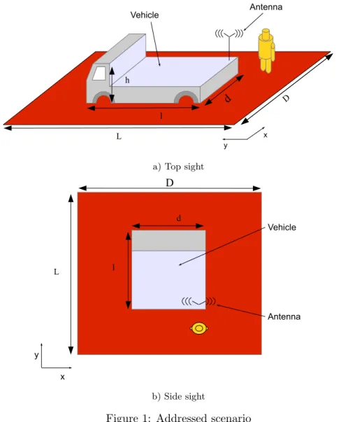
In order to illustrate the new method, we consider the multiscale and variable problem described in figure 1. The purpose is to calculate the electric field in the eye of a whole human body located near an antenna onboard a vehicle.
The human eye diameter is about 2.5 cm whereas the analysed scene has a length and a width of 10.24 m. This very high contrast demonstrates the multiscale feature of the considered problem. The calculation of the field must be carried out for different positions of the person around the vehicle. This aspect reveals the concept of variability.
The vehicle and the person are located in the near field of a monopole antenna matched at the frequency of 60 MHz. We consider this frequency as it is used for military communication systems and, furthermore, the whole body SAR reaches its maximum at this frequency. This shows the need to use a full wave method to analyse the addressed scenario. As the study objective is only to show our method effectiveness the power emitted in the scenario does not correspond to a real system. The amplitude of the transmitter voltage generator is simply fixed to 10 V . The human body model used in the simulations comes from the “Visible Human Project”[16]. It corresponds to the Hugo homogeneous model except eyes which have their own specifications (table 1). The vehicle and the ground are modelled as PEC (Perfect Electric Conductor). The characteristics of the scenario are:
• h = 0.416 × λ60M Hz = 2.08 m,
a) Top sight
b) Side sight
Figure 1: Addressed scenario Table 1: Human body parameters
F=60MHz Permittivity (F/m) Conductivity (S/m)
Human body 0.3970 45.55
Eyes 0.8870 76.68
• l = 0.896 × λ60M Hz = 4.48 m,
• D = L = 2.048 × λ60M Hz = 10.24 m.
3. MACROMODEL BASED DG-FDTD METHOD
The aim of this section is to present the principle and the implementation of the MacroModel based on DG-FDTD method. The building of the substitution model and its insertion in the DG-FDTD method are described.
3.1. Principle of the MM-DG-FDTD method
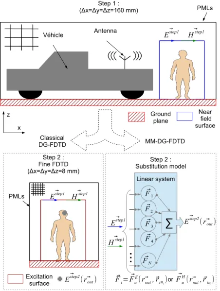
The principle of the MM-DG-FDTD method is to decompose the electromagnetic calculation into two steps performed sequentially (figure 2).
The first step is a coarse FDTD simulation whose objective is to characterize the whole environ-ment including the human body model. The resolution is mainly governed by the smallest considered wavelength. In our case, the body is thus described coarsely. A closed near field surface S is placed around the body in order to store the incident field incoming on the body. This field includes, at a coarse level, all EM interactions between the body and the environment.
In the second step, instead of performing a fine FDTD simulation of the body as in the classic DG-FDTD, the MM-DG-FDTD method proposes to use a rigorous substitution model.
Figure 2: Application of classical DG-FDTD and the MM-DG-FDTD on the addressed scenario Its objective is to compute rigorously and fastly the electric field at one point inside the body and in response to any incident field. In the frequency domain and according to the superposition principle, the model is a linear system.
The input data are the N field components on the near field surface collected in step 1
{ ~Estep1; ~Hstep1}, whereas the output is the electric field at one point in the eye ( ~Estep2) :
Eustep2(~rout) = N X i=1 [ ~FuE(~rout, ~rini). ~E step1(~r ini) + ~F H u (~rout, ~rini). ~H step1(~r ini)] (1) where: • u = x, y or z,
• ~rini belongs to the near field surface S,
• ~rout locates the point in the eye where the output field has to be computed,
• N is the number of cells over the surface S, • ~FE
u and ~FuH are transfer functions.
3.2. Computation of transfer functions
To build the substitution model, an equivalent problem is firstly considered. The field { ~Estep1; ~Hstep1}
on the near field surface S is replaced by surface sources { ~JSstep1; ~MSstep1} using Huygens theory [18]: ~
JSstep1= − ~Hstep1∧ ~n (2)
~
MSstep1= ~Estep1∧ ~n (3)
To determine the transfer functions ~FE
u and ~FuH, a reciprocal problem is considered in which a
source ~JR is located at ~r
out. This source generates a field { ~ER; ~HR}.
In the frequency domain and according to the reciprocity theorem [18], sources and fields of the inital problem are related to those of the reciprocal one as follows:
I S ( ~ER. ~JSstep1− ~HR. ~MSstep1)dS = ZZZ V ( ~Estep2. ~JR)dV (4)
where V is the volume inside the near field surface S. This relation shows that if the fields of the reciprocal problem { ~ER; ~HR} in response to a given ~J
R are known on S then the transfer functions of
equation 1 can be derived easily. To do so, a single fine FDTD simulation of the reciprocal problem is performed. For this simulation, the fine FDTD computation volume is the same as that used in the second step of the classical DG-FDTD (figure 2) but it is excited by the localized electrical source
~ JR(~r
out). During this simulation, { ~ER; ~HR} are recorded on the near field surface S. Expressed in the
frequency domain thanks to FFTs, ~JR, ~ER and ~HR are used to determine the transfer functions as it
is explained below.
For the sake of simplicity, only one face of the near field surface is considered in the following equations. This face is discretized into M cells located. All these cells have equal surface area ∆S and equal unitary normal vectors ~n. The currents are constant on each cell, thus the left side of 4 becomes :
M X i=1 ∆S[ ~ER(~rini). ~J step1 S (~rini) − ~H R(~r ini). ~M step1 S (~rini)] (5)
The source ~JRis oriented along ~e
u and is constant in the FDTD cell of volum ∆V located in ~rout,
thereby, the right side of 4 is given by :
Eustep2(~rout).JuR(~rout)∆V (6)
~ FuE(~rout, ~rini) = − ∆S ∆V . ~n ∧ ~HR(~r ini) JR u(~rout) (7) ~ FuH(~rout, ~rini) = − ∆S ∆V. ~n ∧ ~ER(~r ini) JR u(~rout) (8) One fine FDTD simulation of the reciprocal problem permits to determine the transfer functions { ~FE
u (~rout, ~rini); ~F H
u (~rout, ~rini)}. This single simulation is then enough to determine the field component
Eustep2(~rout) in response to any incident fields { ~Estep1; ~Hstep1} using (1).
3.3. Method overview
The method starts with the computation of transfer functions. In order to determine the three output field components ( ~Estep2(~rout)), it is sufficient to perform three simulations of the reciprocal problem with
the three source orientations : JR
x(~rout), JyR(~rout) and JzR(~rout). The transfer functions can therefore
be calculated and be used again for any incident field { ~Estep1; ~Hstep1}.
Once the transfer functions calculated, the electromagnetic analysis of the addressed scenario for each position of the body is derived as follow
• The first step of the DG-FDTD method is run and the incident fields { ~Estep1; ~Hstep1} is recorded over the near field surface S.
• After being expressed in the frequency domain, the incident field is combined with transfer functions in order to obtain fastly and precisely the desired output field ~Estep2(~rout).
Next section is about the validation of this MM-DG-FDTD method.
4. VALIDATION OF THE MACROMODEL BASED DG-FDTD METHOD
This section presents the validation of the MM-DG-FDTD method. Firstly, a canonical case is considered for the validation of the substitution model. Next, the new method is applied to the addressed scenario of figure 1 in order to assess its performance.
4.1. Validation of the substitution model for a canonical case
To validate the substitution model, a canonical problem is first considered (Figure 3). A volume is illuminated by a z polarized plane wave of amplitude 10 V /m which propagates along the x direction. The time domain excitation covers a 100MHz frequency bandwith ([5;115]MHz). A dielectric block is placed in the simulation box. It has the same specifications as the human body model (table 1). The objective is to estimate the three electric field components at an output point located in the dielectric block. Two simulations are carried out: a standard FDTD one which serves as a reference and a simulation using the substitution model. Table 2 gives the parameters of the reference FDTD simulation and the one used to calculate the transfer functions. The relative difference between the two results is calculated using this relation:
∆Eu(f ) = | Esubs u (f ) − EuF DT D(f ) EF DT D u (f ) | % with : • u = x, y or z, • Esubs
u represents the result for the substitution model,
Figure 3: Canonical case Table 2: Simulation parameters Time Step dt 14.626 ps Spatial resolution (8 × 8 × 8)mm (∆x × ∆y × ∆z) ≈ (λ60M H z 625 )3 mm Volume size (Nx× Ny× Nz) cells (50 × 50 × 30)
Observation time Tobs 200 ns
Figure 4 presents the relative difference between FDTD and substitution model for the three elec-tric field components versus frequency. Even if the substitution model is rigorous, a slight relative error smaller than 2% is observed. This can be explained by the difference in the numerical implementations of the two methods. Anyhow, this agreement is found sufficient for dosimetry applications, as will be shown in the next section.
The analysis of the canonical case has shown that in a simple problem, the substitution model works well. Next subsection assesses its performance in a variable and multiscale problem.
4.2. Application and performance of the MM-DG-FDTD method
We consider the addressed scenario (figure 1) where the aim is to assess the three field components at the center of the eye in response to an illumination resulting from the radiation of an antenna located on a vehicle. The study is done at the frequency of 60 MHz and several positions of the body around the vehicle are considered.
To assess the performance of our approach, a comparison between a classical DG-FDTD and the MM-DG-FDTD method is done. The description of the simulation steps are presented in figure 2. The
20 30 40 50 60 70 80 90 100 110 0 0.2 0.4 0.6 0.8 1 1.2 1.4 1.6 1.8 2 Frequency (MHz) Relative difference (%)
Relative difference for Ex Relative difference for Ey Relative difference for Ez
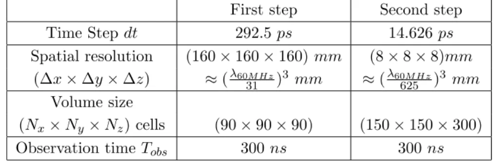
Figure 4: Canonical case’s results: relative difference between FDTD and substitution model Table 3: Simulation parameters of the DG-FDTD method for one position
First step Second step
Time Step dt 292.5 ps 14.626 ps Spatial resolution (160 × 160 × 160) mm (8 × 8 × 8)mm (∆x × ∆y × ∆z) ≈ (λ60M H z 31 )3 mm ≈ ( λ60M H z 625 )3 mm Volume size (Nx× Ny× Nz) cells (90 × 90 × 90) (150 × 150 × 300)
Observation time Tobs 300 ns 300 ns
parameters of the DG-FDTD simulation are reported in table 3. Concerning the new method, the simulation parameters and the computation time associated to the calculation of the transfer functions are given in tables 4 and 5 respectively. The mesh is selected according to the smallest detail in the corresponding computation volume (i.e the eye). Such a grid density is required to describe it with a sufficient accuracy.
Table 4: Simulation parameters of the FDTD simulation used for the calculation of transfer functions Time Step dt 14.626 ps Spatial resolution (8 × 8 × 8)mm (∆x × ∆y × ∆z) ≈ (λ60M H z 625 )3 mm Volume size (Nx× Ny × Nz) cells (150 × 150 × 300)
Observation time Tobs 200 ns
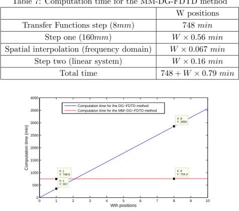
Tables 6 and 7 show the computation time obtained with the two approaches for the study of W different body positions. Compared to a classical DG-FDTD method, the MM-DG-FDTD requires an incompressible 748 min CPU time to calculate the transfer functions. Thus, for a single position study,
Table 5: Computation time for the calculation of transfer functions Simulation time (220 × 3) min
Post-processing 88 min Total time 748 min
Table 6: Computation time for the classical DG-FDTD approach W positions
Step one (160 mm) W × 0.56 min Spatial interpolation (time domain) W × 30 min
Step two (8 mm) W × 326.48 min
Total time W × 357.04 min
Table 7: Computation time for the MM-DG-FDTD method W positions Transfer Functions step (8mm) 748 min
Step one (160mm) W × 0.56 min
Spatial interpolation (frequency domain) W × 0.067 min Step two (linear system) W × 0.16 min
Total time 748 + W × 0.79 min
0 1 2 3 4 5 6 7 8 9 10 0 500 1000 1500 2000 2500 3000 3500 4000 X: 8 Y: 754.3 Wth positions
Computation time (min)
X: 1 Y: 357 X: 1 Y: 748.8 X: 8 Y: 2856
Computation time for the DG−FDTD method Computation time for the MM−DG−FDTD method
Figure 5: Computation time for both methods.
the use of the substitution model is useless compared to the classical DG-FDTD. However, the study of a new position only requires an additionnal 0.79 min CPU time with the new method whereas the additional cost of classical DG-FDTD is 357 min. Therefore, the MM-DG-FDTD method rapidly out-performs the classical DG-FDTD. As figure 5 shows, the use of substitution model presents an interest in terms of calculation time for the study of more than two positions. As an example, an 8-position study requests a time of 2856 min whereas the new method only needs 754.3 min.
It is important to note that the study is done for a single output point. A study conducted on several output points would require more transfer functions and thus an important increase of the com-putation time (748 min for each new output point).
Next section presents a study in which the new method is applied for all possible positions of the addressed scenario.
5. MM-DG-FDTD EXPLOITATION
The MM-DG-FDTD method is applied to analyse the addressed scenario for all possible positions of the body around the vehicle. In the coarse description of the environment, this corresponds to 888
positions and the study is done at the frequency of 60 MHz.
Table 8: Results for one position in the addressed scenario Relative difference between
DG-FDTD and MM-DG-FDTD
|Ex| 0.8526 %
|Ey| 0.48189 %
|Ez| 0.89392 %
|Etotal| 0.73927 %
In order to verify the validity of the MM-DG-FDTD simulation, table 8 compares the results of the classical DG-FDTD simulation with those of the new method for one particular position in the addressed scenario. The MM-DG-FDTD method provides results with an error smaller than 1%.
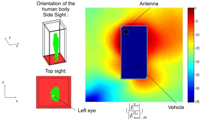
Figure 6: Normalized results using the MM-DG-FDTD.
Figure 6 presents the space orientation of the body and a field cartography. The cartography represents the module of the electric field at the center of the left eye for all 888 positions around
the vehicle. Each pixel gives the amplitude of the electric field in the eye for a given position of the body. For readability, the body is not represented on this map. This cartography is normalized to its maximum. The whole study has been carried out in 1.4495 × 10³ min with the proposed method. For
comparison, it would require 3.1705 × 10⁵ min with the classical DG-FDTD.
6. CONCLUSION.
This paper presents a new method based on the DG-FTD approach. It combines the DG-FDTD method with a substitution model to proceed highly multiscale and variable dosimetric problems. It is demonstrated that the proposed MM-DG-FDTD method provides quick results with a very good accuracy. Reciprocity principle, used in the calculation of transfer functions, works for isotropic materials and passive structures. Furthermore, the DG-FDTD has already been used successfully
to analyse heterogeneous body models [8]. Thus, the MM-DG-FDTD can be also applied to a
heterogeneous body models. To conclude, the MM-DG-FDTD is ready to be used to compute real
life dosimetric problems.
7. CITATIONS REFERENCES
1. ICNIRP website: “http ://www.icnirp.de/documents/emfgdl.pdf ”.
2. A. Taflove and S. C. Hagness, “Computational Electrodynamics: The finite-Difference Time-Domain Method, Third Edition”, Artech House, 2005.
3. A. Johansson, “Wave-propagation from medical implants-influence of body shape on radiation pattern”, Engineering in Medicine and Biology, 24th Annual Conference and the Annual Fall Meeting of the Biomedical Engineering Society EMBS/BMES Conference, 2002. Proceedings of the Second Joint, October 2002, pp. 14091410.
4. J. Wiart, R. Mittra, S. Chaillou, and Z. Altman, “The analysis of human head interaction with a hand-held mobile using the non-uniform FDTD”, Antennas and Propagation for Wireless Communications, IEEE-APS Conference, Nov. 1998, pp. 7780.
5. J.P. Berenger, “A Huygens subgridding for the FDTD method”, IEEE Transactions on Antennas and Propagation Symposium, vol. 54, no.12, pp. 37973804 Dec. 2006.
6. R. A. Chilton and R. Lee, “Explicit 3D FDTD subgridding with provable stability and conservative properties”, IEEE AP-S International Antennas and Propagation Symposium, Honolulu, HI, June 2007, pp. 30693072.
7. R. Pascaud, R. Gillard, R. Loison, J. Wiart and M.F. Wong, “Dual-grid fnite difference time-domains cheme for the fast simulation of surrounded antennas”, IET Microwave Antennas and Propagation, vol. 1, no 3, pages 700706, Juin 2007.
8. C. Miry, R. Loison and R. Gillard, “An Efficient Bilateral Dual-Grid-FDTD Approach Applied to On Body Transmission Analysis and Specifc Absorption Rate Computation , IEEE Transactions on Microwave Theory and Techniques, Vol. 58, No. 9, 2010, pp. 2375-2382.
9. V. Vairavanathan, C. Chang, N. Sood and C.D. Sarris, ”A Reciprocity-Based Framework for the Efficient Modeling of Antenna-Wireless Channel Interaction“, ICEAA 2011, p1271 - 1274, Torino. 10. Omer H. Colak and Ovunc Polat, ”Estimation of local SAR level using RBFNN in threelayer cylindrical human model“, Microwave and Optical Technology Letters, Volume 50, N7, pp 1958-1961, 2008.
11. J.M. Ortiz-Rodriguez, M.R. Martinez-Blanco, E. Gallego and H.R Vega-Carrillo, ”A Computational Tool Design for Evolutionary Artificial Neural Networks in Neutron Spectrometry and Dosimetry“, 2009 Electronics, Robotics and Automotive Mechanics Conference.
12. T. Kientega, E. Conil, A. Hadjem, E. Richalot, A. Gati, M.F. Wong, O. Picon and J. Wiart, ”A surrogate model to assess the whole body SAR induced by multiple plane waves at 2.4 GHz“, Annals of Telecommunications, pp. 419-428, Volume 66, N 7, 2011.
13. Cheol. Hea. Koo. Lee, June. Kyu. Lee and Hyun. Soo. Lim, ”Monte Carlo simulation to measur light dosimetry within the biological tissue“, Proceedings of the 20th Annual International Conference of the IEEE Engineering in Medicine and Biology Society, Vol. 20, No 6, 1998.
14. A. Hirata, O. and Fujiwara, T. Nagaoka and S. Watanabe, ”Estimation of Whole-Body Averaged SARs in Human Models for Far-Field Exposures in Whole-Body Resonance and GHz Frequency Regions“, EMC 2009, Kyoto.
15. A. El Habachi, E. Conil, A. Hadjem, E. Vazquez, M.F. Wong, A. Gati, G. Fleury and J. Wiart, ”Statistical analysis of whole-body absorption depending on anatomical human characteristics at a frequency of 2.1 GHz“, Physics in Medicine and Biology, Volume 55, pp. 1875, 2010.
16. The Visible Human Project: ”http://www.nlm.nih.gov/research/visible/“.
17. O. Aiouaz, D. Lautru, M.F. Wong, E. Conil, A. Gati, J. Wiart and V.F. Hanna, ”Uncertainty analysis of the specific absorption rate induced in a phantom using a stochastic spectral collocation method“, Annals of Telecommunications, pp. 1-10, Volume 66, N7, 2011.
18. Jian-Ming Jin, ”Theory and computation of electromagnetic fields“, IEEE PRESS, chapter 3, p83-87.