Power Modeling on FPGA: A Neural Model for RT-Level Power Estimation

HAL Id: hal-01760342

https://hal.archives-ouvertes.fr/hal-01760342

Submitted on 18 Apr 2018

HAL is a multi-disciplinary open access

archive for the deposit and dissemination of

sci-entific research documents, whether they are

pub-lished or not. The documents may come from

teaching and research institutions in France or

abroad, or from public or private research centers.

L’archive ouverte pluridisciplinaire HAL, est

destinée au dépôt et à la diffusion de documents

scientifiques de niveau recherche, publiés ou non,

émanant des établissements d’enseignement et de

recherche français ou étrangers, des laboratoires

publics ou privés.

Power Modeling on FPGA: A Neural Model for

RT-Level Power Estimation

Yehya Nasser, Jean-Christophe Prevotet, Maryline Hélard

To cite this version:

Yehya Nasser, Jean-Christophe Prevotet, Maryline Hélard. Power Modeling on FPGA: A Neural

Model for RT-Level Power Estimation. ACM International Conference on Computing Frontiers 2018,

May 2018, Ischia, Italy. �10.1145/3203217.3204462�. �hal-01760342�

Estimation

Yehya Nasser, Jean-Christophe Prévotet and Maryline Hélard

Rennes, France yehya.nasser@insa-rennes.fr

ABSTRACT

Today reducing power consumption is a major concern especially when it concerns small embedded devices. Power optimization is required all along the design flow but particularly in the first steps where it has the strongest impact. In this work, we propose new power models based on neural networks that predict the power consumed by digital operators implemented on Field Programmable Gate Arrays (FPGAs). These operators are interconnected and the statistical information of data patterns are propagated among them. The obtained results make an overall power estimation of a specific design possible. A comparison is performed to evaluate the accuracy of our power models against the estimations provided by the Xilinx Power Analyzer (XPA) tool. Our approach is verified at system-level where different processing systems are implemented. A mean absolute percentage error which is less than 8% is shown versus the Xilinx classic flow dedicated to power estimation.

CCS CONCEPTS

• Hardware → Circuits power modeling;

KEYWORDS

Power consumption, power modeling, Neural Network, FPGA

ACM Reference Format:

Yehya Nasser, Jean-Christophe Prévotet and Maryline Hélard. 2018. Power Modeling on FPGA: A Neural Model for RT-Level Power Estimation. In CF ’18: CF ’18: Computing Frontiers Conference, May 8–10, 2018, Ischia, Italy. ACM, New York, NY, USA, 5 pages. https://doi.org/10.1145/3203217.3204462

1

INTRODUCTION

Power consumption has become a critical performance metric in a wide range of electronic devices, from autonomous embedded systems based on batteries to systems requiring a high computing power [10]. Moreover, a huge amount of these devices will clearly have an impact on the environment and on the worldwide energy consumption in particular. One attempt to reduce the consumed power of such devices consists in exploring various hardware ar-chitectures, very soon in the design process, in order to reach an optimal architecture in terms of power consumption. Today, this

exploration is not sufficiently implemented in most of the design tools.

For example, design flows for circuits such as FPGAs do not natively take into consideration power issues at system level. The exploration flow generally consists in implementing several ver-sions of an architecture in the FPGA and get power estimation results after the timing simulation step. Power estimation results are obtained by presenting stimuli data to the circuit and by eval-uating the activity of internal signals. Although very accurate in practice, these results are obtained very late in the design process and require a lot of previous implementation steps, which can be very time consuming. It is also prohibitive when one wants to rapidly test various architectures according to given parameters.

Avoiding hardware implementation for the purpose of estimating the power at early design phases is the best switchable solution for researchers and engineers demanding a faster power estimation at high-level of abstraction. Unfortunately, High Level abstract models are generally not accurate enough and prevent the evaluation and comparison of different hardware solutions.

In our work, we aim to propose a new hardware exploration methodology that tries to combine both accuracy and fast power estimation. This is achieved by estimating the power of specific operators after the hardware implementation on a real platform and by exploiting this information in high-level models. These pre-characterized models can be easily integrated and simulated to estimate the power consumption of an overall design.

This paper particularly focuses on FPGAs targets but the pro-posed methodology may also apply on other hardware targets such as ASICs devices. In FPGAs, the total power consumption has two main contributors i.e static power and dynamic power. Static power is directly related to the transistors leakage current and thus com-pletely technology-dependent. Dynamic power is the power con-sumed in the logic design due to the charging and discharging capacitances when transistors are switching, in addition to the short circuit power. Dynamic power is proportional to the switch-ing activity per clock cycle and is highly data and design dependent. Switching activity has a significant impact on this dynamic power. As in [4], switching activity is a key indicator of dynamic power. The expression of the total power consumption is given in eq. 1

PT otal = PDyn+ PStat = αCV_dd2 f + VddIleakaдe (1) wherePDynis the dynamic power that depends on the switching activity factorα (average numbers of gate transitions per clock cycle), the node capacitanceC, the supply voltage Vdd, and the clock frequency f . The static power PStat is estimated asVdd

Ileakaдe, whereIleakaдe represents the leakage currents.C and Ileakaдeare technology dependent.

CF ’18, May 8–10, 2018, Ischia, Italy Yehya Nasser, Jean-Christophe Prévotet and Maryline Hélard

This paper is organized as follows. Section 2 describes the exist-ing techniques to estimate power consumption. Section 3 describes the proposed method to model and to estimate power. Section 4 illustrates the use of our methodology on different case-studies and provides results and discussions. Finally, section 5 summarizes and concludes the paper.

2

RELATED WORKS

When dealing with design exploration, power modeling becomes a fundamental step that is required for power estimation. Power estimation techniques can be classified into two classes, high-level and low-level approaches. High-level power estimations are based on power models which are used to evaluate power consumption without requiring any implementation and physical details. High-level input parameters are sufficient to obtain a good estimate of the power consumption. The other class deals with low-level power estimation approaches that take into consideration all physical details. These are generally far more accurate as described in [3].

In this paper, we focus on high-level power estimation. In [9], a dynamic power estimation model for FPGA is proposed. It is based on the analytical computation of the switching activity generated inside the components and takes into consideration the correlation between the inputs. A mean relative error of 9.32% for adders and 5.67% for multipliers are obtained compare to measures on a real platform.

A hybrid power modeling approach that accurately and quickly assesses gate-level power consumption is presented in [7]. It con-sists in integrating valuable and accurate physical information with a LUT-based power model to ensure that the correct optimization techniques are implemented. The main disadvantages of the LUT-based macro-modeling are the use of a huge amount of memory to store the input-output statistics and the corresponding simulated power values. Concerning the analytical power models, the main drawback is the simulation time, thereby the need of the computa-tion of the outputs statistics after a time consuming simulacomputa-tion.

Some previous works have introduced artificial intelligence based on neural networks for power estimation. These are described in [2], [8] and [11]. In [2] the neural network is used to estimate the output statistics and the power consumption of complementary metal-oxide-semiconductor (CMOS) circuits. The average absolute relative error of the proposed method is about 5.0%, at circuit level. Using this method, a lot of circuits have to be simulated to cover most applications. Therefore it lacks of generality. In [8], macro-modeling based on neural networks has been applied to different multipliers. A comparison of different models shows that neural networks are the most accurate method over linear equations and LUT-based power estimation models.

Our current work is inspired from [1], and in the continuity of [5] and [6]. In [1] a power macro-model for (Intellectual Property) IP power estimation is proposed that is based on lookup table (LUT) power models. The IP power model used to estimate the power consumption of an IP-based digital system which is based on signal statistics propagation. In [5], IP power models based on neural networks have been proposed. Compare to this previous study, our work aims to consider only operators characterization instead. The idea is to provide a more generic and flexible approach to estimate

power consumption by allowing the design of a complete system from basic operators.

3

POWER ESTIMATION METHODOLOGY

3.1

Proposed approach

The proposed methodology is based on the assumption that any hardware system can be represented by a set of hardware com-ponents that are dedicated to a specific function. The main idea consists in estimating the consumption of a global digital system, based on an accurate power estimation of its sub-components. Each component has been fully characterized and is available in a dedi-cated library.

Once the components have been fully characterized and that accurate models are built, designers have the possibility to construct their architecture by connecting components in a design entry tool that is similar to schematics or with a hardware description language.

The full design may then be simulated at high level to evaluate the performances and obtain an accurate evaluation of the design power profile. Note that, our methodology makes it possible to test various combinations of components and then of architectures very easily, by simply modifying the components in the high level design entry tool. Since our power models are not computation intensive, the simulation results may be obtained very fast, which allows designers to test a lot of configurations in few minutes.

This type of simulation is generally not possible using classical tools since designers need to implement all designs from scratch when a simple modification is performed on the architecture. This may actually lead to several hours or days of simulations to get an accurate power profile of a full design.

In this article, we will focus on describing the characterization phase that aims to develop the power models of different compo-nents. This is explained in the following section.

3.2

Model Definition

The purpose of the characterization phase is to develop a power model of a component by extracting the relevant information that has a direct impact on power. An example of such operator can be a simple component such as an adder, multiplexer, multiplier, decoder, etc. Each operator has its own size and a defined number of inputs and outputs.

In order to evaluate the power consumption of a given circuit, we propose to provide each operator with a power model that depends on the activity rate of its inputs. Each operator model consists actually of two sub-modelsM1 and M2 that are described in Fig. 1. M1 constitutes a first model that predict the power consumption for given (signal rates) SR or (α) and (percentage logic high) PLH or (p) of all inputs. The signal activity of the inputs is expressed in terms of millions of transitions per second (Mtr/sec). For every input, PLH refers to the percentage of time during which the signal is at HIGH level, on a period of 1 s. The global model provides then an average of the energy consumed during this period.

The second sub-model (M2) makes it possible to estimate the signal activity of the outputs as well as the percentage logic high according to the operator’s inputs. This second model is particularly

useful when designers want to propagate the signals’ activity as well as the PLH among all connected operators in their design.

In order to obtain a global power estimation for the entire design, it is then possible to sum-up the power contribution of each opera-tor, at high level. With an accurate estimation of signals activity, these models allow designers to obtain accurate results without spending a lot of time in simulation processes.

As an example, let us consider a system composed ofN opera-tors, and let us assume that the switching activity rate isαi, and thatpi is the percentage logic high at the inputopi of the opera-tor. Therefore, (βi,hi) constitutes the output feature vector of the operator.M1,iandM2,icorresponds to the two models for theopi

input. By propagating this information to the subsequent operators, a global power value can be computed according to eq. 2.

P_Global= M1, 1(α1, p1)+ N −1

Õ

i=2

M1,i(βi−1, hi−1). (2)

Figure 1: Operator Model

3.3

Characterization Process

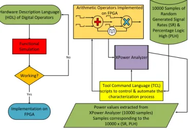
In order to obtain pertinent information regarding the power that is consumed by a specific operator, a characterization phase has to be performed. It consists in implementing the operator on a given FPGA target and in obtaining power results after applying various configurations of SR and PLH values at the operator inputs. This process is performed at low-level of abstraction in order to get as much technical details as possible and to obtain the best accuracy in terms of power estimation. Tools such as XPA may be used to build a huge database that takes into consideration all ranges of signal rates and Percentage Logic High for every inputs. The power characterization process at low-level is described in Fig. 2.

3.4

Neural Network Models

BothM1 and M2 sub-models have been implemented using neural networks that are classical tools that have shown their efficiency in lots of domains. They especially perform very well in classification and also in non-linear regression problems.

Neural networks consist of processing units called neurons that operate in parallel to solve computational problems. In this study, we consider basic multi-layer perceptrons (MLP) feed forward net-works, that permit to model complex behaviors and may perform multi-dimensional functions approximation. Such networks have one or more hidden layers composed of neurons with non linear transfer function, and provide an output layer that implements

Hardware Description Language (HDL) of Digital Operators Functional Simulation Working? No Implementation on FPGA Yes 10000 Samples of Random Generated Signal Rates (SR) & Percentage Logic High (PLH)

Tool Command Language (TCL) scripts to control & automate the

characterization process XPower Analyzer Arithmetic Operators Implemented

on FPGA

Power values extracted from XPower Analyzer (10000 samples)

Samples corresponding to the 10000 x (SR, PLH)

Figure 2: Power characterization Process Description

output neurons with a linear activation function. Fig. 3 shows a typical architecture of an MLP neural network.

In a first learning phase, the multiple layers with nonlinear ac-tivation functions allow the network to learn the relationships between inputs and outputs. This is performed by modifying the weights value between different neurons. In a second phase (the forward phase), the network may estimate the correct output for any given input pattern.

In our models, three layers have been used. Each layer receives its inputs from the precedent layer and forwards its outputs to the subsequent. In the forward phase, the hidden layer weight matrix is multiplied by the input vectorX = (x1, x2, x3, . . . , xn)T, to compute

the hidden layer output, as expressed in equation 3.

yh, j= f Ni Õ i=1 wh, jixi−θ ! (3) wherewh, ji is the weight connecting inputi to unit j in the hidden neuron layer.θ is an offset termed bias that is also connected to each neuron. In order to train the networks, the well known back-propagation algorithm has been used.

Figure 3: MLP Neural Network Architecture

4

EXPERIMENTS AND RESULTS

In order to demonstrate the feasibility of our approach and to quan-tify the models accuracy, case studies have been performed on

CF ’18, May 8–10, 2018, Ischia, Italy Yehya Nasser, Jean-Christophe Prévotet and Maryline Hélard

different arithmetic operators. A full design composed of basic arith-metic operators (adders and multipliers) has been implemented on a xc7z045ffg900 FPGA device.

Two types of power estimation have been performed. The first corresponds to the classic power estimation that is achieved in the last steps of an FPGA design flow (after place and route). Regarding Xilinx FPGAs, this step is implemented using XPA. The second power estimation has been performed using our neural networks models. In this case, simulation is implemented in Matlab and takes place at high-level. The idea is to guarantee a fair comparison between the results obtained with our models and XPA.

Both power estimation types have been achieved on two types of designs. The first consists of a single operator (adder or multiplier) in our case, and the second consists of a more complex combination of these operators i.e an arithmetic function. This aims to demon-strate the use and propagation of signal rates throughout a full design. The results are described in the following sections.

4.1

Per-operator Verification

At operator-level, a verification phase is performed to calculate the accuracy of the proposed models. As shown in Fig. 4, XPA has been used to estimate the power consumption of a 16 bit adder and a 16 bit multiplier. For the same operators, the MATLAB tool has then been used to estimate the dynamic power consumption using the neural approach.

By providing the 16 bit adder / 16 bit multiplier with 10000 sam-ples of signal rates and PLH, then 10000 data-samsam-ples of dynamic power have been extracted from XPA. The exact same inputs given to XPA are also provided to the neural models to evaluate both power consumption and the signal rate and PLH. BothM1 and M2 neural networks have thus 16 (bits) x 2 (inputs) x 2 (signal rates + PLH) = 64 inputs. Both models respectively contains 100 and 150 nodes in their hidden layer. The training set of each neural network consists of 64x10000 data-samples (80% for training, 10% for valida-tion and 10% for testing) with different combinavalida-tions of signal rates and PLH. At the output of theM1 Neural Network, only one power value is provided. TheM2 Neural Network provides 16 (bits)x 2 (signal rates + PLH) = 32 outputs to propagate the signal activity to other subsequent models. BothM1 and M2 models are grouped in a single block that is described in Fig. 4.

Op

X1 X2

Data_out Neural Network Operator Model Data_in_16-bit 32xSR_in 32xPLH_in Estimated Power 16xSR_out 16xPLH_out

Figure 4: Neural network accuracy measurements Table 1 shows the relative error at operator-level in terms of power estimation. The relative error has been calculated according to 10000 data samples.

The results shown in this table indicate a relative error that is very small (around 0.01%). This shows that neural networks have learned the behavior of XPA and are able to model it very accurately.

Operators Real Power Modeled Power Relative Error (mW) (mW) (%) Adder 1.7879 1.7881 0.0112 Multiplier 27.4147 27.4136 0.0040

Table 1: Power accuracy for the considered models

4.2

Per-system Verification

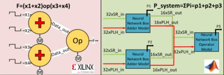
At system-level, verification of several scenarios have been per-formed. Figure 5 describes a function composed of single operators. As in the per-operator approach, XPA has been used to evaluate the power of the global system as well as the SR and PLH parameters. In parallel, another global model has been built under Matlab and consists in interconnecting bothM1 and M2 models for each oper-ator and perform an high-Level simulation. This simulation aims to propagate the parameters throughout all operators and provides an overall power estimation.

F=(x1+x2)op(x3+x4) X1 X2 X3 X4 Op F Neural Network Box Adder Model Neural Network Box Adder Model Neural Network Box Operator Model P_system=ΣPi=p1+p2+p3 P1 P2 P3 16xPLH_out 16xPLH_out 16xSR_out 32xSR_in 32xPLH_in 32xSR_in 32xPLH_in 16xSR_out 32xSR_in 32xPLH_in

Figure 5: System level power estimation XPA vs NN For both simulations, the same inputs, signal rates and PLH combinations of 5000 data-samples have been provided to both XPA and neural models. 5000 data-samples of dynamic power values have been extracted from XPA and from the global neural power models. Note that two functions have been implemented :Fi = (a

opb) op (c op d), where op can either be an adder or a multiplier. As in eq. 4, a mean absolute percentage error is calculated over 5000 data samples at system-level to evaluate the accuracy of the approach.PX PAis the power consumption calculated using the XPA tool andPN N is the power consumption estimated by the power model. %MAPESystem−level=100_n n Õ i=1 |PX PA−P_{N N}| PX PA (4)

Arithmetic Function Neural models (MAPE %) F1(op1=+, op2=+, op3=+) 7.3699

F2(op1=*, op2=*, op3=*) 3.5158

Table 2: Models Accuracy for Different Functions

According to the results given in Table 2, it can be seen that our method provides a good accuracy at system-level with an error that is less than 8%.

Table 3 shows the initial estimates that are based on the sum of the total average power of each operator. These estimates exhibit

Arithmetic XPA-based Initial Relative Error Function (mw) Estimates (mw) (%)

F1 4.6282 5.3637 15.8965 F2 70.2986 82.2441 16.9925 Table 3: The effect of Signal Activity Propagation Versus Ini-tial Estimates

low accurate results, with a relative error that is greater than 15%. Two sources of errors can be identified :first, the SR modeling errors propagate and accumulate through the full design. Second, in XPA, the fact that operators are connected to several neighbors has a direct impact on the impedance and thus on the power consumption. Note that power consumption of the intra-connections (within an operator) is taken into consideration in each neural model.

These results show that it is necessary to take into account signal propagation between operators for more accurate estimation.

4.3

Exploration Time

The purpose of this section is demonstrate the feasibility of our ap-proach that consists in using high-level models to improve designs’ exploration time.

We propose to compare our approach with the classic FPGA design flow that makes it possible to obtain an accurate power estimation of a full design. To this aim, we considered the simple example that is provided in section 4.2. In order to underline the impact of the exploration time, let us consider that designers decide to start implementing arithmetic function F1. We would like to eval-uate the overhead that is required to obtain new power estimation results if the design is modified to implement another function, let say, function F2.

Using the Xilinx classic design flow, designers have to re-run the complete flow and run the XPA estimation tool for the new F2 version. In this case, the design entry has to be modified accordingly and synthesis and implementation steps are required. Moreover, designers have to run the XPA power estimation tool to get a new power of estimation. Although quite fast in this simple example, it is important to note that these steps may become prohibitive when dealing with complex systems with a lot of components. Changing a single component demands to run the complete flow for the modified design.

With our approach, designers only need to modify the instances in the design entry tool and perform a high-level simulation with SystemC. No additional steps are required. Furthermore, power estimation is completely integrated in the simulator tool that can perform complex simulations in a very fast time (less than few seconds).

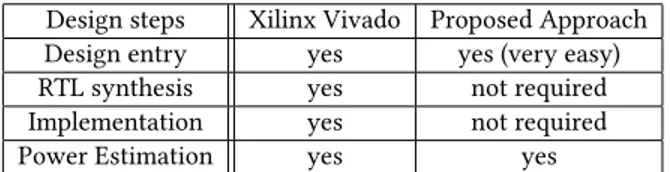
The different design steps that need to be followed are summa-rized in table 4.

5

CONCLUSION

In this work, we have presented a new methodology, in which neu-ral networks are the key models used for High-Level estimation of the consumed power. Two types of neural networks have been used to estimate power and signal activity (signal rate and PLH). Both

Design steps Xilinx Vivado Proposed Approach Design entry yes yes (very easy) RTL synthesis yes not required Implementation yes not required Power Estimation yes yes

Table 4: Required design steps to switch from F1 to F2 con-figurations

types show a very good accuracy when considering simple opera-tors. When using these models to evaluate more complex functions, the obtained results are less accurate on the power estimation due to the fact of the modeling errors and the interconnections power. In a near future, we aim to develop a library of high-level power models dedicated to FPGAs that can be jointly used with high-level design tools to help designers in optimizing their systems. Our work will make it possible to simulate a design very rapidly without implementing architectures from scratch. Moreover, a real measurement bench will be constructed to measure the power con-sumption on the FPGA core. Using the measured power values for specific operators to model the power consumption will help us in developing more accurate models.

REFERENCES

[1] Durrani Yaseer Arafat and Riesgo Teresa. 2014. Power Estimation for Intellectual Property-based Digital Systems at the Architectural Level. J. King Saud Univ. Comput. Inf. Sci. 26, 3 (Sept. 2014), 287–295. https://doi.org/10.1016/j.jksuci.2014. 03.005

[2] W. Q. Y. Cao, Yuanyuan Yan, and Xun Gao. 2005. Neural Network Macromodel for High-Level Power Estimation of CMOS Circuits. In 2005 International Conference on Neural Networks and Brain, Vol. 2. 1009–1014. https://doi.org/10.1109/ICNNB. 2005.1614789

[3] Li Fei, Chen Deming, He Lei, and Cong Jason. 2003. Architecture Evaluation for Power-efficient FPGAs. In Proceedings of the 2003 ACM/SIGDA Eleventh Inter-national Symposium on Field Programmable Gate Arrays (FPGA ’03). ACM, New York, NY, USA, 175–184. https://doi.org/10.1145/611817.611844

[4] E. Hung, J. J. Davis, J. M. Levine, E. A. Stott, P. Y. K. Cheung, and G. A. Constan-tinides. 2016. KAPow: A System Identification Approach to Online Per-Module Power Estimation in FPGA Designs. In 2016 IEEE 24th Annual International Symposium on Field-Programmable Custom Computing Machines (FCCM). 56–63. https://doi.org/10.1109/FCCM.2016.25

[5] J. Lorandel, J. C. Prévotet, and M. Hélard. 2016. Efficient modelling of FPGA-based IP blocks using neural networks. In 2016 International Symposium on Wireless Communication Systems (ISWCS). 571–575. https://doi.org/10.1109/ISWCS.2016. 7600969

[6] Y. Nasser, J. C. Prévotet, M. Hélard, and J. Lorandel. 2017. Dynamic power estimation based on switching activity propagation. In 2017 27th International Conference on Field Programmable Logic and Applications (FPL). 1–2. https: //doi.org/10.23919/FPL.2017.8056783

[7] A. Nocua, A. Virazel, A. Bosio, P. Girard, and C. Chevalier. 2016. A Hybrid Power Estimation Technique to improve IP power models quality. In 2016 IFIP/IEEE International Conference on Very Large Scale Integration (VLSI-SoC). 1–6. https: //doi.org/10.1109/VLSI-SoC.2016.7753582

[8] K. Roy. 2007. Neural Network Based Macromodels for High Level Power Estima-tion. In International Conference on Computational Intelligence and Multimedia Applications (ICCIMA 2007), Vol. 2. 159–163. https://doi.org/10.1109/ICCIMA. 2007.117

[9] Jevtic Ruzica and Carreras Carlos. 2012. A Complete Dynamic Power Estimation Model for Data-paths in FPGA DSP Designs. Integr. VLSI J. 45, 2 (March 2012), 172–185. https://doi.org/10.1016/j.vlsi.2011.09.002

[10] A. Suissa, O. Romain, J. Denoulet, K. Hachicha, and P. Garda. 2010. Empirical Method Based on Neural Networks for Analog Power Modeling. IEEE Transactions on Computer-Aided Design of Integrated Circuits and Systems 29, 5 (May 2010), 839–844. https://doi.org/10.1109/TCAD.2010.2043759

[11] G. Zhou, B. Guo, X. Gao, J. Ma, H. He, and Y. Yan. 2015. A FPGA Power Estima-tion Method Based on an Improved BP Neural Network. In 2015 InternaEstima-tional Conference on Intelligent Information Hiding and Multimedia Signal Processing (IIH-MSP). 251–254. https://doi.org/10.1109/IIH-MSP.2015.76