HAL Id: hal-01711595
https://hal.archives-ouvertes.fr/hal-01711595
Submitted on 19 Feb 2018
HAL is a multi-disciplinary open access
archive for the deposit and dissemination of
sci-entific research documents, whether they are
pub-lished or not. The documents may come from
teaching and research institutions in France or
L’archive ouverte pluridisciplinaire HAL, est
destinée au dépôt et à la diffusion de documents
scientifiques de niveau recherche, publiés ou non,
émanant des établissements d’enseignement et de
recherche français ou étrangers, des laboratoires
Adapting Consistency in Constraint Solving
Amine Balafrej, Christian Bessière, Anastasia Paparrizou, Gilles Trombettoni
To cite this version:
Amine Balafrej, Christian Bessière, Anastasia Paparrizou, Gilles Trombettoni. Adapting Consistency
in Constraint Solving. Christian Bessiere; Luc De Raedt; Lars Kotthoff; Siegfried Nijssen; Barry
O’Sullivan; Dino Pedreschi. Data Mining and Constraint Programming - Foundations of a
Cross-Disciplinary Approach, LNCS (10101), Springer, pp.226-253, 2016, 978-3-319-50136-9.
�10.1007/978-3-319-50137-6_9�. �hal-01711595�
Adapting Consistency in Constraint Solving
⇤
Amine Balafrej
1Christian Bessiere
2Anastasia Paparrizou
2Gilles Trombettoni
21
TASC (INRIA/CNRS), Mines Nantes, France
2
CNRS, University of Montpellier, France
Abstract
State-of-the-art constraint solvers uniformly maintain the same level of local consistency (usually arc consistency) on all the instances. We propose two approaches to adjust the level of consistency depending on the instance and on which part of the instance we propagate. The first ap-proach, parameterized local consistency, uses as parameter the stability of values, which is a feature computed by arc consistency algorithms during their execution. Parameterized local consistencies choose to enforce arc consistency or a higher level of local consistency to a value depending on whether the stability of the value is above or below a given threshold. In the adaptive version, the parameter is dynamically adapted during search, and so is the level of local consistency. In the second approach, we focus on partition-one-AC, a singleton-based consistency. We propose adap-tive variants of partition-one-AC that do not necessarily run until having proved the fixpoint. The pruning can be weaker than the full version, but the computational e↵ort can be significantly reduced. Our experiments show that adaptive parameterized maxRPC and adaptive partition-one-AC can obtain significant speed-ups over arc consistency and over the full versions of maxRPC and partition-one-AC.
1
Introduction
Enforcing local consistency by applying constraint propagation during search is one of the strengths of constraint programming (CP). It allows the constraint solver to remove locally inconsistent values. This leads to a reduction of the search space. Arc consistency is the oldest and most well-known way of propa-gating constraints [Bes06]. It has the nice feature that it does not modify the structure of the constraint network. It just prunes infeasible values. Arc con-sistency is the standard level of concon-sistency maintained in constraint solvers.
⇤The results contained in this chapter have been presented in [BBCB13] and [BBBT14]. This work has been funded by the EU project ICON (FP7-284715).
Several other local consistencies pruning only values and stronger than arc con-sistency have been proposed, such as max restricted path concon-sistency or single-ton arc consistency [DB97]. These local consistencies are seldom used in prac-tice because of the high computational cost of maintaining them during search. However, on some instances of problems, maintaining arc consistency is not a good choice because of the high number of ine↵ective revisions of constraints that penalize the CPU time. For instance, Stergiou observed that when solving the scen11, an instance from the radio link frequency assignment problem (RL-FAP) class, with an algorithm maintaining arc consistency, only 27 out of the 4103 constraints of the problem were identified as causing a domain wipe-out and 1921 constraints did not prune any value [Ste09].
Choosing the right level of local consistency for solving a problem requires finding a good trade-o↵ between the ability of this local consistency to remove inconsistent values, and the cost of the algorithm that enforces it. The works of [Ste08] and [PS12] suggest to take advantage of the power of strong propagation algorithms to reduce the search space while avoiding the high cost of maintaining them in the whole network. These methods result in a heuristic approach based on the monitoring of propagation events to dynamically adapt the level of local consistency (arc consistency or max restricted path consistency) to individual constraints. This prunes more values than arc consistency and less than max restricted path consistency. The level of propagation obtained is not character-ized by a local consistency property. Depending on the order of propagation, we can converge on di↵erent closures. In other work, a high level of consistency is applied in a non exhaustive way, because it is very expensive when applied exhaustively everywhere in the network during the whole search. In [SS09], a preprocessing phase learns which level of consistency to apply on which parts of the instance. When dealing with global constraints, some authors propose to weaken arc consistency instead of strengthening it. In [KVH06], Katriel et al. proposed a randomized filtering scheme for AllDi↵erent and Global Cardi-nality Constraint. In [Sel03], Sellmann introduced the concept of approximated consistency for optimization constraints and provided filtering algorithms for Knapsack Constraints based on bounds with guaranteed accuracy.
In this chapter, we propose two approaches for adapting automatically the level of consistency during search. Our first approach is based on the notion of stability of values. This is an original notion independent of the characteristics of the instance to be solved, but based on the state of the arc consistency algo-rithm during its propagation. Based on this notion, we propose parameterized consistencies, an original approach to adjust the level of consistency inside a given instance. The intuition is that if a value is hard to prove arc consistent (i.e., the value is not stable for arc consistency), this value will perhaps be pruned by a stronger local consistency. The parameter p specifies the threshold of stability of a value v below which we will enforce a stronger consistency to v. A parameterized consistency p-LC is thus an intermediate level of consis-tency between arc consisconsis-tency and another consisconsis-tency LC, stronger than arc consistency. The strength of p-LC depends on the parameter p. This approach allows us to find a trade-o↵ between the pruning power of local consistency and
the computational cost of the algorithm that achieves it. We apply p-LC to the case where LC is max restricted path consistency. We describe the algorithm p-maxRPC3 (based on p-maxRPC3 [BPSW11]) that achieves p-max restricted path consistency. Then, we propose ap-LC, an adaptive variant of p-LC that uses the number of failures in which variables or constraints are involved to assess the difficulty of the di↵erent parts of the problem during search. ap-LC dynamically and locally adapts the level p of local consistency to apply depending on this difficulty.
Our second approach is inspired by singleton-based consistencies. They have been shown extremely efficient to solve some classes of hard problems [BCDL11]. Singleton-based consistencies apply the singleton test principle, which consists of assigning a value to a variable and trying to refute it by enforcing a given level of consistency. If a contradiction occurs during this singleton test, the value is removed from its domain. The first example of such a local consistency is Singleton Arc Consistency (SAC), introduced in [DB97]. In SAC, the single-ton test enforces arc consistency. By definition, SAC can only prune values in the variable domain on which it currently performs singleton tests. In [BA01], Partition-One-AC (which we call POAC) has been proposed. POAC is an ex-tension of SAC that can prune values everywhere in the network as soon as a variable has been completely singleton tested. As a consequence, the fixpoint in terms of filtering is often quickly reached in practice. This observation has already been made on numerical constraint problems. In [TC07,NT13], a con-sistency called Constructive Interval Disjunction (CID), close to POAC in its principle, gave good results by simply calling the main procedure once on each variable or by adapting during search the number of times it is called. Based on these observations, we propose an adaptive version of POAC, called APOAC, where the number of times variables are processed for singleton tests on their values is dynamically and automatically adapted during search. A sequence of singleton tests on all values of one variable is called a varPOAC call. The number k of times varPOAC is called will depend on how e↵ective POAC is or not in pruning values. This number k of varPOAC calls will be learned during a sequence of nodes of the search tree (learning nodes) by measuring stagnation in the amount of pruned values. This amount k of varPOAC calls will be applied at each node during a sequence of nodes (called exploitation nodes) before we enter a new learning phase to adapt k again. Observe that if the number of varPOACcalls learned is 0, then adaptive POAC will mimic AC.
The aim of both of the proposed adaptive approaches (i.e., ap-LC and APOAC) is to adapt the level of consistency automatically and dynamically during search. ap-LC uses failure information to learn what are the most diffi-cult parts of the problem and it increases locally and dynamically the parameter p on those difficult parts. APOAC measures a stagnation in number of inconsis-tent values removed for k calls of varPOAC. APOAC then uses this information to stop enforcing POAC. APOAC avoids the cost of the last calls to varPOAC that delete very few values or no value at all. We thus see that both ap-LC and APOAC learn some information during search to adapt the level of consistency. This allows them to benefit from the pruning power of a high level of consistency
while avoiding the prohibitive time cost of fully maintaining this high level. The rest of the paper is organized as follows. Section2contains the necessary formal background. Section3describes the parameterized consistency approach and gives an algorithm for parameterized maxRPC. In Section4, the adaptive variant of parameterized consistency is defined. Sections5and6are devoted to our study of singleton-based consistencies. In Section5, we propose an efficient POAC algorithm that will be used as a basis for the adaptive versions of POAC. Section6 presents di↵erent ways to learn the number of variables on which to perform singleton tests. All these sections contain experimental results that validate the di↵erent contributions. Section7concludes this work.
2
Background
A constraint network is defined as a set of n variables X = {x1, ..., xn}, a
set of ordered domains D = {D(x1), ..., D(xn)}, and a set of e constraints
C = {c1, ..., ce}. Each constraint ck is defined by a pair (var(ck), sol(ck)),
where var(ck) is an ordered subset of X, and sol(ck) is a set of combinations
of values (tuples) satisfying ck. In the following, we restrict ourselves to binary
constraints, because the local consistency (maxRPC) we use here to instanti-ate our approach is defined on the binary case only. However, the notions we introduce can be extended to non-binary constraints, by using maxRPWC for instance [BSW08]. A binary constraint c between xi and xj will be denoted by
cij, and (xi) will denote the set of variables xj involved in a constraint with
xi.
A value vj 2 D(xj) is called an arc consistent support (AC support) for
vi2 D(xi) on cij if (vi, vj)2 sol(cij). A value vi2 D(xi) is arc consistent (AC)
if and only if for all xj 2 (xi) vi has an AC support vj 2 D(xj) on cij. A
domain D(xi) is arc consistent if it is non empty and all values in D(xi) are arc
consistent. A network is arc consistent if all domains in D are arc consistent. If enforcing arc consistency on a network N leads to a domain wipe out, we say that N is arc inconsistent.
A tuple (vi, vj)2 D(xi)⇥D(xj) is path consistent (PC) if and only if for any
third variable xk there exists a value vk2 D(xk) such that vk is an AC support
for both vi and vj. In such a case, vk is called witness for the path consistency
of (vi, vj).
A value vj 2 D(xj) is a max restricted path consistent (maxRPC) support
for vi 2 D(xi) on cij if and only if it is an AC support and the tuple (vi, vj)
is path consistent. A value vi 2 D(xi) is max restricted path consistent on
a constraint cij if and only if there exist vj 2 D(xj) maxRPC support for vi
on cij. A value vi 2 D(xi) is max restricted path consistent ifand only if for
all xj 2 (xi) vi has a maxRPC support vj 2 D(xj) on cij. A variable xi is
maxRPC if its domain D(xi) is non empty and all values in D(xi) are maxRPC.
A network is maxRPC if all domains in D are maxRPC.
A value vi 2 D(xi) is singleton arc consistent (SAC) if and only if the
incon-sistent. A variable xi is SAC if D(xi)6= ; and all values in D(xi) are SAC. A
network is SAC if all its variables are SAC.
A variable xi is partition-one-AC (POAC) if and only if D(xi) 6= ;, all
values in D(xi) are SAC, and 8j 2 1..n, j 6= i, 8vj 2 D(xj), 9vi 2 D(xi) such
that vj 2 AC(N|xi=vi). A constraint network N = (X, D, C) is POAC if and
only if all its variables are POAC. Observe that POAC, as opposed to SAC, is able to prune values from all variable domains when being enforced on a given variable.
Following [DB97], we say that a local consistency LC1 is stronger than a
local consistency LC2 (LC2 LC1) if LC2 holds on any constraint network on
which LC1 holds. It has been shown in [BA01] that POAC is strictly stronger
than SAC. Hence, SAC holds on any constraint network on which POAC holds and there exist constraint networks on which SAC holds but not POAC.
The problem of deciding whether a constraint network has solutions is called the constraint satisfaction problem (CSP), and it is NP-complete. Solving a CSP is mainly done by backtrack search that maintains some level of consistency between each branching step.
3
Parameterized Consistency
In this section, we present an original approach to parameterize a level of consis-tency LC stronger than arc consisconsis-tency so that it degenerates to arc consisconsis-tency when the parameter equals 0, to LC when the parameters equals 1, and to levels in between when the parameter is between 0 and 1. The idea behind this is to be able to adjust the level of consistency to the instance to be solved, hoping that such an adapted level of consistency will prune significantly more values than arc consistency while being less time consuming than LC.
Parameterized consistency is based on the concept of stability of values. We first need to define the ’distance to end’ of a value in a domain. This captures how far a value is from the last in its domain. In the following, rank(v, S) is the position of value v in the ordered set of values S.
Definition 1 (Distance to end of a value) The distance to end of a value vi2 D(xi) is the ratio
(xi, vi) = (|Do(xi)| rank(vi, Do(xi)))/|Do(xi)|,
where Do(xi) is the initial domain of xi.
We see that the first value in Do(xi) has distance (|Do(xi)| 1)/|Do(xi)|
and the last one has distance 0. Thus,8vi2 D(xi), 0 (xi, vi) < 1.
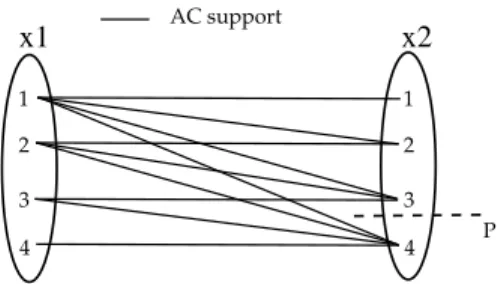
We can now give the definition of what we call the parameterized stability of a value for arc consistency. The idea is to define stability for values based on the distance to the end of their AC supports. For instance, consider the constraint x1 x2with the domains D(x1) = D(x2) ={1, 2, 3, 4} (see Figure1).
x1 x2 1 2 3 4 AC support P 1 2 3 4
Figure 1: Stability of supports on the example of the constraint x1 x2 with
the domains D(x1) = D(x2) ={1, 2, 3, 4}. (x1, 4) is not p-stable for AC.
If p = 0.2, the value (x1, 4) is not p-stable for AC, because the first and only
AC support of (x1, 4) in the ordering used to look for supports, that is (x2, 4),
has a distance to end smaller than the threshold p. Proving that the pair (4, 4) is inconsistent (by a stronger consistency) could lead to the pruning of (x1, 4).
In other words, applying a stronger consistency on (x1, 4) has a higher chance
to lead to its removal than applying it to for instance (x1, 1), which had no
difficulty to find its first AC support (distance to end of (x2, 1) is 0.75).
At this point, we want to emphasize that the ordering of values used to look for supports in the domains is not related to the order in which values are selected by the branching heuristic used by the backtrack search procedure. That is, we can use a given order of values for looking for supports and another one for exploring the search tree.
Definition 2 (p-stability for AC) A value vi 2 D(xi) is p-stable for AC on
cij i↵ vi has an AC support vj2 D(xj) on cij such that (xj, vj) p. A value
vi2 D(xi) is p-stable for AC i↵ 8xj2 (xi), vi is p-stable for AC on cij.
We are now ready to give the first definition of parameterized local consis-tency. This first definition can be applied to any local consistency LC for which the consistency of a value on a constraint is well defined. This is the case for instance for all triangle-based consistencies [DB01, Bes06].
Definition 3 (Constraint-based p-LC) Let LC be a local consistency stronger than AC for which the LC consistency of a value on a constraint is defined. A value vi2 D(xi) is constraint-based p-LC on cij i↵ it is p-stable for
AC on cij, or it is LC on cij. A value vi2 D(xi) is constraint-based p-LC i↵
8cij, viis constraint-based p-LC on cij. A constraint network is constraint-based
p-LC i↵ all values in all domains in D are constraint-based p-LC.
Theorem 1 Let LC be a local consistency stronger than AC for which the LC consistency of a value on a constraint is defined. Let p1and p2be two parameters
in [0..1]. If p1< p2, then AC constraint-based p1-LC constraint-based p2
Proof. Suppose that there exist two parameters p1, p2such that 0 p1< p2
1, and suppose that there exists a p2-LC constraint network N that contains
a p2-LC value (xi, vi) that is p1-LC inconsistent. Let cij be the constraint on
which (xi, vi) is p1-LC inconsistent. Then, @vj 2 D(xj) that is an AC support
for (xi, vi) on cij such that (xj, vj) p1. Thus, vi is not p2-stable for AC on
cij. In addition, vi is not LC on cij. Therefore, vi is not p2-LC, and N is not
p2-LC.
Definition 3 can be modified to a more coarse-grained version that is not dependent on the consistency of values on a constraint. This will have the advantage to apply to any type of strong local consistency, even those, like singleton arc consistency, for which the consistency of a value on a constraint is not defined.
Definition 4 (Value-based p-LC) Let LC be a local consistency stronger than AC. A value vi 2 D(xi) is value-based p-LC if and only if it is p-stable
for AC or it is LC. A constraint network is value-based p-LC if and only if all values in all domains in D are value-based p-LC.
Theorem 2 Let LC be a local consistency stronger than AC. Let p1 and p2 be
two parameters in [0..1]. If p1< p2then AC value-based p1-LC value-based
p2-LC LC.
Proof. Suppose that there exist two parameters p1, p2such that 0 p1< p2
1, and suppose that there exists a p2-LC constraint network N that contains a
p2-LC value (xi, vi) that is p1-LC-inconsistent. vi is p1-LC-inconsistent means
that:
1. vi is not p1-stable for AC:9cij on which vi is not p1-stable for AC. Then
@vj2 D(xj) that is an AC support for (xi, vi) on cijsuch that (xj, vj)
p1. Therefore, vi is not p2-stable for AC on cij, then vi is not p2-stable
for AC.
2. vi is LC inconsistent.
(1) and (2) imply that vi is not p2-LC and N is not p2-LC.
For both types of definitions of p-LC, we have the following property on the extreme cases (p = 0, p = 1).
Corollary 1 Let LC1 and LC2 be two local consistencies stronger than AC.
We have: value-based 0-LC2 = AC and value-based 1-LC2 = LC. If the LC1
consistency of a value on a constraint is defined, we also have: constraint-based 0-LC1= AC and constraint-based 1-LC1= LC.
3.1
Parameterized maxRPC: p-maxRPC
To illustrate the benefit of our approach, we apply parameterized consistency to maxRPC to obtain the p-maxRPC level of consistency that achieves a consis-tency level between AC and maxRPC.
Algorithm 1: Initialization(X, D, C, Q) 1 begin 2 foreach xi2 X do 3 foreach vi2 D(xi) do 4 foreach xj2 (xi) do 5 p-support false; 6 foreach vj2 D(xj) do 7 if (vi, vj)2 cij then 8 LastACxi,vi,xj vj; 9 if (xj, vj) p then 10 p-support true; 11 LastP Cxi,vi,xj vj; 12 break; 13 if searchPCwit(vi, vj) then 14 p-support true; 15 LastP Cxi,vi,xj vj; 16 break; 17 if ¬p-support then 18 remove vifrom D(xi); 19 Q Q [ {xi}; 20 break;
21 if D(xi) =; then return false;
22 return true;
Definition 5 (p-maxRPC) A value is p-maxRPC if and only if it is constraint-based p-maxRPC. A network is p-maxRPC if and only if it is constraint-based p-maxRPC.
From Theorem1 and Corollary1 we derive the following corollary.
Corollary 2 For any two parameters p1, p2, 0 p1 < p2 1, AC p1
-maxRP C p2-maxRP C maxRP C. 0-maxRP C = AC and 1-maxRP C =
maxRP C.
We propose an algorithm for p-maxRPC, based on maxRPC3, the best exist-ing maxRPC algoritm. We do not describe maxRPC3 in full detail, as it can be found in [BPSW11]. We only describe procedures where changes to maxRPC3 are necessary to design p-maxRPC3, a coarse grained algorithm that performs p-maxRPC. We use light grey to emphasize the modified parts of the original maxRPC3 algorithm.
maxRPC3 uses a propagation list Q where it inserts the variables whose domains have changed. It also uses two other data structures: LastAC and LastPC. For each value (xi, vi), LastACxi,vi,xj stores the smallest AC support
Algorithm 2: checkPCsupLoss(vj, xi) 1 begin 2 if LastACxj,vj,xi2 D(xi) then 3 bi max(LastP Cxj,vj,xi+1,LastACxj,vj,xi); 4 else 5 bi max(LastP Cxj,vj,xi+1,LastACxj,vj,xi+1); 6 foreach vi2 D(xi), vi bido 7 if (vj, vi)2 cji then
8 if LastACxj,vj,xi2 D(x/ i) & LastACxj,vj,xi>LastP Cxj,vj,xi then 9 LastACxj,vj,xi vi; 10 if (xi, vi) p then 11 LastP Cxj,vj,xi vi; 12 return true; 13 if searchPCwit(vj, vi) then 14 LastP Cxj,vj,xi vi; 15 return true; 16 return f alse;
on cij (i.e., the smallest AC support (xj, vj) for (xi, vi) on cij such that (vi, vj)
is PC). This algorithm comprises two phases: initialization and propagation. In the initialization phase (algorithm 1) maxRPC3 checks if each value (xi, vi) has a maxRPC-support (xj, vj) on each constraint cij. If not, it
re-moves vi from D(xi) and inserts xi in Q. To check if a value (xi, vi) has a
maxRPC-support on a constraint cij, maxRPC3 looks first for an AC-support
(xj, vj) for (xi, vi) on cij, then it checks if (vi, vj) is PC. In this last step, changes
were necessary to obtain p-maxRPC3 (lines 9-12). We check if (vi, vj) is PC
(line 13) only if (xj, vj) is smaller than the parameter p (line 9).
The propagation phase of maxRPC3 involves propagating the e↵ect of dele-tions. While Q is non empty, maxRPC3 extracts a variable xi from Q and
checks for each value (xj, vj) of each neighboring variable xj 2 (xi) if it is
not maxRPC because of deletions of values in D(xi). A value (xj, vj) becomes
maxRPC inconsistent in two cases: if its unique PC-support (xi, vi) on cij has
been deleted, or if we deleted the unique witness (xi, vi) for a pair (vj, vk) such
that (xk, vk) is the unique PC-support for (xj, vj) on cjk. So, to propagate
deletions, maxRPC3 checks if the last maxRPC support (last known support) of (xj, vj) on cij still belongs to the domain of xi, otherwise it looks for the next
support (algorithm 2). If such a support does not exist, it removes the value vj and adds the variable xj to Q. Then if (xj, vj) has not been removed in the
previous step, maxRPC3 checks (algorithm 3) whether there is still a witness for each pair (vj, vk) such that (xk, vk) is the PC support for (xj, vj) on cjk. If
not, it looks for the next maxRPC support for (xj, vj) on cjk. If such a support
Algorithm 3: checkPCwitLoss(xj, vj, xi) 1 begin 2 foreach xk2 (xj)\ (xi) do 3 witness false; 4 if vk LastP Cxj,vj,xk2 D(xk) then 5 if (xk, vk) p then 6 witness true; 7 else
8 if LastACxj,vj,xi2 D(xi) & LastACxj,vj,xi=LastACxk,vk,xi 9 ORLastACxj,vj,xi2 D(xi) & ( LastACxj,vj,xi, vk)2 cik 10 ORLastACxk,vk,xi2 D(xi) & ( LastACxk,vk,xi, vj)2 cij
11 then witness true ;
12 else
13 if searchACsup(xj, vj, xi) & searchACsup(xk, vk, xi) then
14 foreach vi2 D(xi), vi max(LastACxj,vj,xi,LastACxk,vk,xi) do 15 if (vj, vi)2 cji& (vk, vi)2 cki then 16 witness true; 17 break;
18 if ¬witness & ¬checkPCsupLoss(vj, xk) then return f alse ;
19 return true;
In the propagation phase, we also modified maxRPC3 to check if the values are still p-maxRPC instead of checking if they are maxRPC. In p-maxRPC3, the last p-maxRPC support for (xj, vj) on cij is the last AC support if (xj, vj)
is p-stable for AC on cij. If not, it is the last PC support. Thus, p-maxRPC3
checks if the last p-maxRPC support (last known support) of (xj, vj) on cij
still belongs to the domain of xi. If not, it looks (algorithm 2) for the next
AC support (xi, vi) on cij, and checks if (vi, vj) is PC (line 13) only when
(xi, vi) < p (line 10). If no p-maxRPC support exists, p-maxRPC3 removes
the value and adds the variable xj to Q. If the value (xj, vj) has not been
removed in the previous phase, p-maxRPC3 checks (algorithm 3) whether there is still a witness for each pair (vj, vk) such that (xk, vk) is the p-maxRPC support
for vj on cjk and (xk, vk) < p. If not, it looks for the next p-maxRPC support
for vj on cjk. If such a support does not exist, it removes vj from D(xj) and
adds the variable xj to Q.
p-maxRPC3 uses the data structure LastP C to store the last p-maxRPC support (i.e., the latest AC support for the p-stable values and the latest PC support for the others). Algorithms1and2update the data structure LastP C of maxRPC3 to be LastAC for all the values that are p-stable for AC (line 11
of Algorithm 1 and line 11 of Algorithm 2) and avoid seeking witnesses for those values. Algorithm3 avoids checking the loss of witnesses for the p-stable
values by setting the flag witness to true (line 6). Correctness of p-maxRPC3 directly comes from maxRPC3: The removed values are necessarily p-maxRPC-inconsistent and all the values that are p-maxRPC-p-maxRPC-inconsistent are removed.
3.2
Experimental validation of p-maxRPC
To validate the approach of parameterized local consistency, we conducted a first basic experiment. The purpose of this experiment is to see if there exist instances on which a given level of p-maxRPC, with a value p that is uniform (i.e., identical for the entire constraint network) and static (i.e., constant through the entire search process), is more efficient than AC or maxRPC, or both.
We have implemented the algorithms that achieve p-maxRPC as described in the previous section in our own binary constraint solver, in addition to maxRPC (maxRPC3 version [BPSW11]) and AC (AC2001 version [BRYZ05]). All the al-gorithms are implemented in our JAVA CSP solver.We tested these alal-gorithms on several classes of CSP instances from the International Constraint Solver Competition 091. We have only selected instances involving binary constraints. To isolate the e↵ect of propagation, we used the lexicographic ordering for vari-ables and values. We set the CPU timeout to one hour. Our experiments were conducted on a 12-core Genuine Intel machine with 16Gb of RAM running at 2.92GHz.
On each instance of our experiment, we ran AC, max-RPC, and p-maxRPC for all values of p in{0.1, 0.2, . . . , 0.9}. Performance has been measured in terms of CPU time in seconds, the number of visited nodes (NODE) and the number of constraint checks (CCK). Results are presented as ”CPU time (p)”, where p is the parameter for which p-maxRPC gives the best result.
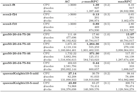
Table 1 reports the performance of AC, maxRPC, and p-maxRPC for the value of p producing the best CPU time, on instances from Radio Link Frequency Assignment Problems (RLFAPs), geom problems, and queens knights problems. The CPU time of the best algorithm is bold-faced. On RLFAP and geom, we observe the existence of a parameter p for which p-maxRPC is faster than both AC and maxRPC for most instances of these two classes of problems. On the queens-knight problem, however, AC is always the best algorithm. In Figures
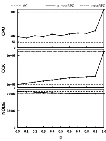
2 and 3, we try to understand more closely what makes p-maxRPC better or worse than AC and maxRPC. Figures 2 and 3 plot the performance (CPU, NODE and CCK) of p-maxRPC for all values of p from 0 to 1 by steps of 0.1 against performance of AC and maxRPC. Figure 2 shows an instance where p-maxRPC solves the problem faster than AC and maxRPC for values of p in the range [0.3..0.8]. We observe that p-maxRPC is faster than AC and maxRPC when it reduces the size of the search space as much as maxRPC (same number of nodes visited) with a number of CCK closer to the number of CCK produced by AC. Figure3shows an instance where the CPU time for p-maxRPC is never better than both AC and maxRPC, whatever the value of p. We see that p-maxRPC is two to three times faster than p-maxRPC. But p-p-maxRPC fails to
Table 1: Performance (CPU time, nodes and constraint checks) of AC, p-maxRPC, and maxRPC on various instances.
AC p-maxRPC maxRPC scen1-f8 CPU >3600 1.39 (0.2) 6.10 #nodes – 927 917 #ccks – 1,397,440 26,932,990 scen2-f24 CPU >3600 0.13 (0.3) 0.65 #nodes – 201 201 #ccks – 296,974 3,462,070 scen3-f10 CPU >3600 0.89 (0.5) 2.80 #nodes – 469 408 #ccks – 874,930 13,311,797 geo50-20-d4-75-26 CPU 111.48 17.80 (1.0) 15.07 #nodes 477,696 3,768 3,768 #ccks 96,192,822 40,784,017 40,784,017 geo50-20-d4-75-43 CPU 1,671.35 1,264.36 (0.5) 1,530.02 #nodes 4,118,134 555,259 279,130 #ccks 1,160,664,461 1,801,402,535 3,898,964,831 geo50-20-d4-75-46 CPU 1,732.22 371.30 (0.6) 517.35 #nodes 3,682,394 125,151 64,138 #ccks 1,516,856,615 584,743,023 1,287,674,430 geo50-20-d4-75-84 CPU 404.63 0.44 (0.6) 0.56 #nodes 2,581,794 513 333 #ccks 293,092,144 800,657 1,606,047 queensKnights10-5-add CPU 27.14 30.79 (0.2) 98.44 #nodes 82,208 81,033 78,498 #ccks 131,098,933 148,919,686 954,982,880 queensKnights10-5-mul CPU 43.89 83.27 (0.1) 300.74 #nodes 74,968 74,414 70,474 #ccks 104,376,698 140,309,576 1,128,564,278
improve AC because the number of constraint checks performed by p-maxRPC is much higher than the number of constraint checks performed by AC, whereas the number of nodes visited by p-maxRPC is not significantly reduced compared to the number of nodes visited by AC. From these observations, it thus seems that p-maxRPC outperforms AC and maxRPC when it finds a compromise between the number of nodes visited (the power of maxRPC) and the number of CCK needed to maintain (the light cost of AC).
In Figures 2 and 3 we can see that the CPU time for 1-maxRPC (respec-tively 0-maxRPC) is greater than the CPU time for maxRPC (respec(respec-tively AC), although the two consistencies are equivalent. The reason is that p-maxRPC performs tests on the distances. For p = 0, we also explain this di↵erence by the fact that p-maxRPC maintains data structures that AC does not use.
4
Adaptative Parameterized Consistency:
ap-maxRPC
In the previous section, we have defined p-maxRPC, a version of parameterized consistency where the strong local consistency is maxRPC. We have performed some initial experiments where p has the same value during the whole search and
Figure 2: Instance where p-maxRPC outperforms both AC and maxRPC.
Figure 3: Instance where AC outper-forms p-maxRPC.
everywhere in the constraint network. However, the algorithm we proposed to enforce p-maxRPC does not specify how p is chosen. In this section, we propose two possible ways to dynamically and locally adapt the parameter p in order to solve the problem faster than both AC and maxRPC. Instead of using a single value for p during the whole search and for the whole constraint network, we propose to use several local parameters and to adapt the level of local consistency by dynamically adjusting the value of the di↵erent local parameters during search. The idea is to concentrate the e↵ort of propagation by increasing the level of consistency in the most difficult parts of the given instance. We can determine these difficult parts using heuristics based on conflicts in the same vein as the weight of a constraint or the weighted degree of a variable in [BHLS04].
4.1
Constraint-based ap-maxRPC : apc-maxRPC
The first technique we propose, called constraint-based ap-maxRPC, assigns a parameter p(ck) to each constraint ck in C. We define this parameter to be
correlated to the weight of the constraint. The idea is to apply a higher level of consistency in parts of the problem where the constraints are the most active. Definition 6 (The weight of a constraint [BHLS04]) The weight w(ck)
of a constraint ck 2 C is an integer that is incremented every time a domain
wipe-out occurs while performing propagation on this constraint.
We define the adaptive parameter p(ck) local to constraint ck in such a way
8ck 2 C, p(ck) = w(ck) minc2C(w(c))
maxc2C(w(c)) minc2C(w(c)) (1)
Equation1 is normalized so that we are guaranteed that 0 p(ck) 1 for
all ck2 C and that there exists ck1 with p(ck1) = 0 (the constraint with lowest
weight) and ck2 with p(ck2) = 1 (the constraint with highest weight).
We are now ready to define adaptive parameterized consistency based on constraints.
Definition 7 (constraint-based ap-maxRPC) A value vi 2 D(xi) is
constraint-based ap-maxRPC (or apc-maxRPC) on a constraint cij if and only
if it is constraint-based p(cij)-maxRPC. A value vi2 D(xi) is apc-maxRPC i↵
8cij, vi is apc-maxRPC on cij. A constraint network is apc-maxRPC i↵ all
values in all domains in D are apc-maxRPC.
4.2
Variable-based ap-maxRPC: apx-maxRPC
The technique proposed in Section4.1can only be used on consistencies where the consistency of a value on a constraint is defined. We present a second tech-nique which can be used on constraint-based or variable-based local consisten-cies indi↵erently. We instantiate our definitions to maxRPC but the extension to other consistencies is direct. We call this new technique variable-based ap-maxRPC. We need to define the weighted degree of a variable as the aggregation of the weights of all constraints involving it.
Definition 8 (The weighted degree of a variable [BHLS04]) The weighted degree wdeg(xi) of a variable xi is the sum of the weights of the
constraints involving xi and one other uninstantiated variable.
We associate each variable with an adaptive local parameter based on its weighted degree.
8xi 2 X, p(xi) =
wdeg(xi) minx2X(wdeg(x))
maxx2X(wdeg(x)) minx2X(wdeg(x))
(2) As in Equation 1, we see that the local parameter is normalized so that we are guaranteed that 0 p(xi) 1 for all xi2 X and that there exists xk1 with
p(xk1) = 0 (the variable with lowest weighted degree) and xk2 with p(xk2) = 1
(the variable with highest weighted degree).
Definition 9 (variable-based ap-maxRPC) A value vi2 D(xi) is
variable-based ap-maxRPC (or apx-maxRPC) if and only if it is value-variable-based p(xi
)-maxRPC. A constraint network is apx-maxRPC i↵ all values in all domains in D are apx-maxRPC.
4.3
Experimental evaluation of ap-maxRPC
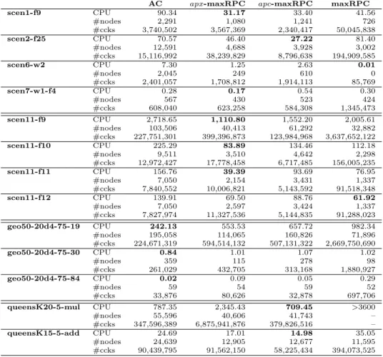
In Section3.2we have shown that maintaining a static form of p-maxRPC during the entire search can lead to a promising trade-o↵ between computational e↵ort and pruning when all algorithms follow the same static variable ordering. In this section, we want to put our contributions in the real context of a solver using the best known variable ordering heuristic, dom/wdeg, though it is known that this heuristic is so good that it substantially reduces the di↵erences in performance that other features of the solver could provide. We have compared the two variants of adaptive parameterized consistency, namely apc-maxRPC and apx-maxRPC, to AC and maxRPC. We ran the four algorithms on instances of radio link frequency assignment problems, geom problems, and queens knights problems.
Table 2 reports some representative results. A first observation is that, thanks to the dom/wdeg heuristic, we were able to solve more instances before the cuto↵ of one hour, especially the scen11 variants of RLFAP. A second ob-servation is that apc-maxRPC and apx-maxRPC are both faster than at least one of the two extreme consistencies (AC and maxRPC) on all instances except scen7-w1-f4 and geo50-20-d4-75-30. Third, when apx-maxRPC and/or apc-maxRPC are faster than both AC and apc-maxRPC (scen1-f9, scen2-f25, scen11-f9, scen11-f10 and scen11-f11), we observe that the gap in performance in terms of nodes and CCKs between AC and maxRPC is significant. Except for scen7-w1-f4, the number of nodes visited by AC is three to five times greater than the number of nodes visited by maxRPC and the number of constraint checks performed by maxRPC is twelve to sixteen times greater than the number of constraint checks performed by AC. For the geom instances the CPU time of the ap-maxRPC algorithms is between AC and maxRPC, and it is never lower than the CPU time of AC. This probably means that when solving these in-stances with the dom/wdeg heuristic, there is no need for sophisticated local consistencies. In general we see that the ap-maxRPC algorithms fail to improve both the two extreme consistencies simultaneously for the instances where the performance gap between AC and maxRPC is low.
If we compare maxRPC to apc-maxRPC, we observe that although apx-maxRPC is coarser in its design than apc-apx-maxRPC, apx-apx-maxRPC is often faster than apc-maxRPC. We can explain this by the fact that the constraints initially all have the same weight equal to 1. Hence, all local parameters ap(ck) initially
have the same value 0, so that apc-maxRPC starts resolution by applying AC everywhere. It will start enforcing some amount of maxRPC only after the first wipe-out occurred. On the contrary, in apx-maxRPC, when constraints all have the same weight, the local parameter p(xi) is correlated to the degree of
the variable xi. As a result, apx-maxRPC benefits from the filtering power of
maxRPC even before the first wipe-out.
In Table2, we reported only the results on a few representative instances. Table 3 summarizes the entire set of experiments. It shows the average CPU time for each algorithm on all instances of the di↵erent classes of problems tested. We considered only the instances solved before the cuto↵ of one hour
Table 2: Performance (CPU time, nodes and constraint checks) of AC, variable-based ap-maxRPC (apx-maxRPC), constraint-based ap-maxRPC (apc-maxRPC), and maxRPC on various instances.
AC apx-maxRPC apc-maxRPC maxRPC scen1-f9 CPU 90.34 31.17 33.40 41.56 #nodes 2,291 1,080 1,241 726 #ccks 3,740,502 3,567,369 2,340,417 50,045,838 scen2-f25 CPU 70.57 46.40 27.22 81.40 #nodes 12,591 4,688 3,928 3,002 #ccks 15,116,992 38,239,829 8,796,638 194,909,585 scen6-w2 CPU 7.30 1.25 2.63 0.01 #nodes 2,045 249 610 0 #ccks 2,401,057 1,708,812 1,914,113 85,769 scen7-w1-f4 CPU 0.28 0.17 0.54 0.30 #nodes 567 430 523 424 #ccks 608,040 623,258 584,308 1,345,473 scen11-f9 CPU 2,718.65 1,110.80 1,552.20 2,005.61 #nodes 103,506 40,413 61,292 32,882 #ccks 227,751,301 399,396,873 123,984,968 3,637,652,122 scen11-f10 CPU 225.29 83.89 134.46 112.18 #nodes 9,511 3,510 4,642 2,298 #ccks 12,972,427 17,778,458 6,717,485 156,005,235 scen11-f11 CPU 156.76 39.39 93.69 76.95 #nodes 7,050 2,154 3,431 1,337 #ccks 7,840,552 10,006,821 5,143,592 91,518,348 scen11-f12 CPU 139.91 69.50 88.76 61.92 #nodes 7,050 2,597 3,424 1,337 #ccks 7,827,974 11,327,536 5,144,835 91,288,023 geo50-20d4-75-19 CPU 242.13 553.53 657.72 982.34 #nodes 195,058 114,065 160,826 71,896 #ccks 224,671,319 594,514,132 507,131,322 2,669,750,690 geo50-20d4-75-30 CPU 0.84 1.01 1.07 1.02 #nodes 359 115 278 98 #ccks 261,029 432,705 313,168 1,880,927 geo50-20d4-75-84 CPU 0.02 0.09 0.05 0.29 #nodes 59 54 59 52 #ccks 33,876 80,626 32,878 697,706 queensK20-5-mul CPU 787.35 2,345.43 709.45 >3600 #nodes 55,596 40,606 41,743 – #ccks 347,596,389 6,875,941,876 379,826,516 – queensK15-5-add CPU 24.69 17.01 14.98 35.05 #nodes 24,639 12,905 12,677 11,595 #ccks 90,439,795 91,562,150 58,225,434 394,073,525
by at least one of the four algorithms. To compute the average CPU time of an algorithm on a class of instances, we add the CPU time needed to solve each instance solved before the cuto↵ of one hour, and for the instances not solved before the cuto↵, we add one hour. We observe that the adaptive approach is, on average, faster than the two extreme consistencies AC and maxRPC, except on the geom class.
In apx-maxRPC and apc-maxRPC, we update the local parameters p(xi) or
p(ck) at each node in the search tree. We could wonder if such a frequent update
does not produce too much overhead. To answer this question we performed a simple experiment in which we update the local parameters every 10 nodes
Table 3: Average CPU time of AC, variable-based ap-maxRPC (apx-maxRPC), constraint-based ap-maxRPC (apc-maxRPC), and maxRPC on all instances of each class of problems tested, when the local parameters are updated at each node
class (#instances) AC apx-maxRPC apc-maxRPC maxRPC geom (10) #solved 10 10 10 10 average CPU 69.28 180.57 191.03 279.30 scen (10) #solved 10 10 10 10 average CPU 18.95 9.63 8.30 13.94 scen11 (10) #solved 4 4 4 4 average CPU 810.15 325.90 467.28 564.17 queensK (11) #solved 6 6 6 5 average CPU 135.95 395.41 121.75 >610.51
Table 4: Average CPU time of AC, variable-based ap-maxRPC (apx-maxRPC), constraint-based ap-maxRPC (apc-maxRPC), and maxRPC on all instances of each class of problems tested, when the local parameters are updated every 10 nodes
class (#instances) AC apx-maxRPC apc-maxRPC maxRPC geom (10) #solved 10 10 10 10 average CPU 69.28 147.20 189.42 279.30 scen (10) #solved 10 10 10 10 average CPU 18.95 7.40 8.86 13.94 scen11 (10) #solved 4 4 4 4 average CPU 810.15 311.74 417.97 564.17 queensK (11) #solved 6 6 6 5 average CPU 135.95 269.51 117.18 >610.52
only. We re-ran the whole set of experiments with this new setting. Table 4
reports the average CPU time for these results. We observe that when the local parameters are updated every 10 nodes, the gain for the adaptive approach is, on average, greater than when the local parameters are updated at each node. This gives room for improvement, by trying to adapt the frequency of update of these parameters.
5
Partition-One-Arc-Consistency
In this section, we describe our second approach, which is inspired from singleton-based consistencies. Singleton Arc Consistency (SAC) [DB97] makes a singleton test by enforcing arc consistency and can only prune values in the vari-able domain on which it currently performs singleton tests. Partition-One-AC (POAC) [BA01] is an extension of SAC, which, as observed in [BD08], combines singleton tests and constructive disjunction [VSD98]. POAC can prune values everywhere in the network as soon as a variable has been completely singleton tested.
vari-ables are processed for singleton tests on their values is dynamically and auto-matically adapted during search. Before moving to adaptive partition-one-AC, we first propose an efficient algorithm enforcing POAC and we compare its behaviour to SAC.
5.1
The algorithm
The efficiency of our POAC algorithm, POAC1, is based on the use of counters associated with each value (xj, vj) in the constraint network. These counters
are used to count how many times a value vjfrom a variable xjis pruned during
the sequence of POAC tests on all the values of another variable xi(the varPOAC
call to xi). If vj is pruned|D(xi)| times, this means that it is not POAC and
can be removed from D(xj).
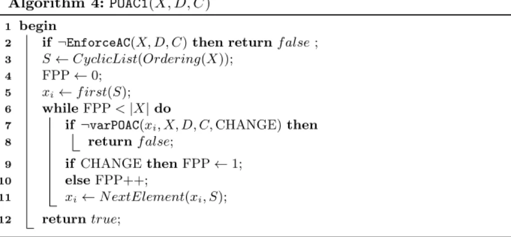
POAC1(Algorithm4) starts by enforcing arc consistency on the network (line
2). Then it puts all variables in the ordered cyclic list S using any total ordering on X (line3). varPOAC iterates on all variables from S (line7) to make them POAC until the fixpoint is reached (line12) or a domain wipe-out occurs (line
8). The counter FPP (FixPoint Proof) counts how many calls to varPOAC have been processed in a row without any change in any domain (line9).
The procedure varPOAC (Algorithm 5) is called to establish POAC w.r.t. a variable xi. It works in two steps. The first step enforces arc consistency in
each sub-network N = (X, D, C[ {xi= vi}) (line4) and removes vi from D(xi)
(line5) if the sub-network is arc-inconsistent. Otherwise, the procedure TestAC (Algorithm 6) increments the counter associated with every arc inconsistent value (xj, vj), j 6= i in the sub-network N = (X, D, C [ {xi = vi}). (Lines 6
and 7 have been added for improving the performance in practice but are not necessary for reaching the required level of consistency.) In line8 the Boolean CHANGE is set to true if D(xi) has changed. The second step deletes all the
values (xj, vj), j6= i with a counter equal to |D(xi)| and sets back the counter
of each value to 0 (lines12-13). Whenever a domain change occurs in D(xj),
if the domain is empty, varPOAC returns failure (line14); otherwise it sets the Boolean CHANGE to true (line15).
Enforcing arc consistency on the sub-networks N = (X, D, C[ {xi = vi})
is done by calling the procedure TestAC (Algorithm 6). TestAC just checks whether arc consistency on the sub-network N = (X, D, C[ {xi= vi}) leads to
a domain wipe-out or not. It is an instrumented AC algorithm that increments a counter for all removed values and restores them all at the end. In addition to the standard propagation queue Q, TestAC uses a list L to store all the removed values. After the initialisation of Q and L (lines2-3), TestAC revises each arc (xj, ck) in Q and adds each removed value (xj, vj) to L (lines5-10). If
a domain wipe-out occurs (line11), TestAC restores all removed values (line12) without incrementing the counters (call to RestoreDomains with UPDATE = f alse) and it returns failure (line13). Otherwise, if values have been pruned from the revised variable (line 14) it puts in Q the neighbouring arcs to be revised. At the end, removed values are restored (line16) and their counters are incremented (call to RestoreDomains with UPDATE = true) before returning
Algorithm 4: POAC1(X, D, C)
1 begin
2 if ¬EnforceAC(X, D, C) then return false ;
3 S CyclicList(Ordering(X)); 4 FPP 0;
5 xi first(S);
6 while FPP <|X| do
7 if ¬varPOAC(xi, X, D, C, CHANGE) then
8 return f alse; 9 if CHANGE then FPP 1; 10 else FPP++; 11 xi NextElement(xi, S); 12 return true; success (line17).
Proposition 1 POAC1 has a worst-case time complexity in O(n2d2(T + n)),
where T is the time complexity of the arc-consistency algorithm used for sin-gleton tests, n is the number of variables, and d is the number of values in the largest domain.
Proof. The cost of calling varPOAC on a single variable is O(dT + nd) because varPOACruns AC on d values and updates nd counters. In the worst case, each of the nd value removals trigger n calls to varPOAC. Therefore POAC1 has a time
complexity in O(n2d2(T + n)). ⇤
5.2
Comparison of POAC and SAC behaviors
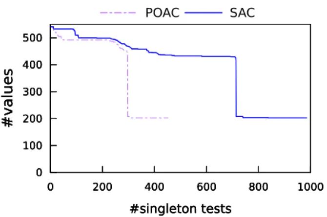
Although POAC has a worst-case time complexity greater than SAC, we ob-served in practice that maintaining POAC during search is often faster than maintaining SAC. This behavior occurs even when POAC cannot remove more values than SAC, i.e. when the same number of nodes is visited with the same static variable ordering. This is due to what we call the (filtering) convergence speed : when both POAC and SAC reach the same fixpoint, POAC reaches the fixpoint with fewer singleton tests than SAC.
Figure 4 compares the convergence speed of POAC and SAC on an CSP instance where they have the same fixpoint. We observe that POAC is able to reduce the domains, to reach the fixpoint, and to prove the fixpoint, all in fewer singleton tests than SAC. This pattern has been observed on most of the instances and whatever ordering was used in the list S. The reason is that each time POAC applies varPOAC to a variable xi, it is able to remove inconsistent
values from D(xi) (like SAC), but also from any other variable domain (unlike
Algorithm 5: varPOAC(xi, X, D, C, CHANGE) 1 begin
2 SIZE |D(xi)|; CHANGE false;
3 foreach vi2 D(xi) do
4 if ¬TestAC(X, D, C [ {xi= vi}) then
5 remove vifrom D(xi);
6 if ¬EnforceAC(X, D, C, xi) then return f alse ;
7 if D(xi) =; then return false;
8 if SIZE6= |D(xi)| then CHANGE true;
9 foreach xj2 X\{xi} do
10 SIZE |D(xj)|;
11 foreach vj2 D(xj) do
12 if counter(xj, vj) =|D(xi)| then remove vjfrom D(xj) ;
13 counter(xj, vj) 0;
14 if D(xj) =; then return false;
15 if SIZE6= |D(xj)| then CHANGE true;
16 return true
The fact that SAC cannot remove values in variables other than the one on which the singleton test is performed makes it a poor candidate for adapting the number of singleton tests. A SAC-inconsistent variable/value pair never singleton tested has no chance to be pruned by such a technique.
6
Adaptive POAC
This section presents an adaptive version of POAC that approximates POAC by monitoring the number of variables on which to perform singleton tests.
To achieve POAC, POAC1 calls the procedure varPOAC until it has proved that the fixpoint is reached. This means that, when the fixpoint is reached, POAC1 needs to call n (additional) times the procedure varPOAC without any pruning to prove that the fixpoint was reached. Furthermore, we experimentally observed that in most cases there is a long sequence of calls to varPOAC that prune very few values, even before the fixpoint has been reached (see Figure4
as an example). The goal of Adaptive POAC (APOAC) is to stop iterating on varPOAC as soon as possible. We want to benefit from strong propagation of singleton tests while avoiding the cost of the last calls to varPOAC that delete very few values or no value at all.
6.1
Principle
The APOAC approach alternates between two phases during search: a short learning phase and a longer exploitation phase. One of the two phases is exe-cuted on a sequence of nodes before switching to the other phase for another
Algorithm 6: TestAC(X, D, C[ {xi= vi}) 1 begin
2 Q {(xj, ck)| ck2 (xi), xj2 var(ck), xj6= xi} ;
3 L ; ;
4 while Q6= ; do
5 pick and delete (xj, ck) from Q ;
6 SIZE |D(xj)| ; 7 foreach vj2 D(xj) do 8 if ¬HasSupport(xj, vj, ck) then 9 remove vj from D(xj) ; 10 L L [ (xj, vj) ; 11 if D(xj) =; then 12 RestoreDomains(L, f alse) ; 13 return f alse ; 14 if |D(xj)| < SIZE then 15 Q Q [ {(xj0, ck0)|ck02 (xj), xj0 2 var(ck0), xj0 6= xj, ck0 6= ck}; 16 RestoreDomains(L, true) ; 17 return true ;
sequence of nodes. The search starts with a learning phase. The total length of a pair of sequences learning + exploitation is fixed to the parameter LE.
Before providing a more detailed description, let us define the (log2 of the)
volume of a constraint network N = (X, D, C), used to approximate the size of the search space:
V = log2 n
Y
i=1
|D(xi)|
We use the logarithm of the volume instead of the volume itself, because of the large integers the volume generates. We also could have used the perimeter (i.e., Pi|D(xi)|) for approximating the search space size, as done in [NT13].
Algorithm 7: RestoreDomains(L, UPDATE)
1 begin 2 if UPDATE then 3 foreach (xj, vj)2 L do 4 D(xj) D(xj)[ {vj} ; 5 counter(xj, vj) counter(xj, vj) + 1 ; 6 else 7 foreach (xj, vj)2 L do 8 D(xj) D(xj)[ {vj} ;
0 100 200 300 400 500 0 200 400 600 800 1000 # v a lu es #singleton tests 0 100 200 300 400 500 0 200 400 600 800 1000 # v a lu es #singleton tests 0 100 200 300 400 500 0 200 400 600 800 1000 # v a lu es #singleton tests POAC SAC
Figure 4: The convergence speed of POAC and SAC.
However, experiments have confirmed that the volume is a more precise and e↵ective criterion for adaptive POAC.
The ith learning phase is applied to a sequence of L = 101 · LE consecutive nodes. During that phase, we learn a cuto↵ value ki, which is the maximum
number of calls to the procedure varPOAC that each node of the next (ith) exploitation phase will be allowed to perform. A good cuto↵ ki is such that
varPOACremoves many inconsistent values (that is, obtains a significant volume reduction in the network) while avoiding calls to varPOAC that delete very few values or no value at all. During the ith exploitation phase, applied to a sequence of 9
10· LE consecutive nodes, the procedure varPOAC is called at each node until
fixpoint is proved or the cuto↵ limit of ki calls to varPOAC is reached.
The ith learning phase works as follows. Let ki 1 be the cuto↵ learned at
the previous learning phase. We initialize maxK to max(2· ki 1, 2). At each
node nj in the new learning sequence n1, n2, . . . nL, APOAC is used with a
cuto↵ maxK on the number of calls to the procedure varPOAC. APOAC stores the sequence of volumes (V1, . . . , Vlast), where Vp is the volume resulting from
the pth call to varPOAC and last is the smallest among maxK and the number of calls needed to prove fixpoint. Once the fixpoint is proved or the maxKth call to varPOAC performed, APOAC computes ki(j), the number of varPOAC
calls that are enough to sufficiently reduce the volume while avoiding the extra cost of the last calls that remove few or no value. (The criteria to decide what ’sufficiently’ means are described in Section 6.2.) Then, to make the learning phase more adaptive, maxK is updated before starting node nj+1. If ki(j) is
close to maxK, that is, greater than 3
4· maxK, we increase maxK by 20%. If
ki(j) is less than 12 · maxK, we reduce maxK by 20%. Otherwise, maxK is
unchanged. Once the learning phase ends, APOAC computes the cuto↵ ki that
will be applied to the next exploitation phase. ki is an aggregation of the ki(j)
values, j = 1, ..., L, computed using one of the aggregation techniques presented in Section6.3.
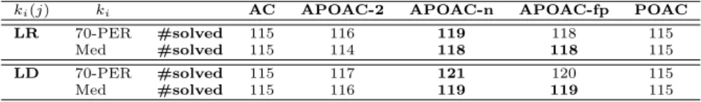
Table 5: Total number of instances solved by AC, several variants of APOAC, and POAC.
ki(j) ki AC APOAC-2 APOAC-n APOAC-fp POAC LR 70-PER #solved 115 116 119 118 115
Med #solved 115 114 118 118 115 LD 70-PER #solved 115 117 121 120 115 Med #solved 115 116 119 119 115
6.2
Computing k
i(j)
We implemented APOAC using two di↵erent techniques to compute ki(j) at a
node nj of the learning phase:
• LR (Last Reduction) ki(j) is the rank of the last call to varPOAC that
reduced the volume of the constraint network.
• LD (Last Drop) ki(j) is the rank of the last call to varPOAC that has
produced a significant drop of the volume. The significance of a drop is captured by a ratio 2 [0, 1]. More formally, ki(j) = max{p | Vp
(1 )Vp 1}.
6.3
Aggregation of the k
i(j) values
Once the ith learning phase is complete, APOAC aggregates the ki(j) values
computed during that phase to generate ki, the new cuto↵ value on the number
of calls to the procedure varPOAC allowed at each node of the ith exploitation phase. We propose two techniques to aggregate the ki(j) values into ki.
• Med ki is the median of the ki(j), j2 1..L.
• q-PER This technique generalizes the previous one. Instead of taking the median, we use any percentile. That is, ki is equal to the smallest value
among ki(1), . . . , ki(L) such that q% of the values among ki(1), . . . , ki(L)
are less than or equal to ki.
Several variants of APOAC can be proposed, depending on how we compute the ki(j) values in the learning phase and how we aggregate the di↵erent ki(j)
values. In the next section, we give an experimental comparison of the di↵erent variants we tested.
6.4
Experimental evaluation of (A)POAC
This section presents experiments that compare the performance of maintaining AC, POAC, or adaptive variants of POAC during search. For the adaptive variants we use two techniques to determine ki(j): the last reduction (LR) and
Table 6: CPU time for AC, APOAC-2, APOAC-n, APOAC-fp and POAC on the eight problem classes.
class (#instances) AC APOAC-2 APOAC-n APOAC-fp POAC
Tsp-20 (15) #solved 15 15 15 15 15 sum CPU 1,596.38 3,215.07 4,830.10 7,768.33 18,878.81 Tsp-25 (15) #solved 15 14 15 15 11 sum CPU 20,260.08 >37,160.63 16,408.35 33,546.10 >100,947.01 renault (50) #solved 50 50 50 50 50 sum CPU 837.72 2,885.66 11,488.61 15,673.81 18,660.01 cril (8) #solved 4 5 7 7 7 sum CPU >45,332.55 >42,436.17 747.05 876.57 1,882.88 mug (8) #solved 5 6 6 6 6 sum CPU >29,931.45 12,267.39 12,491.38 12,475.66 2,758.10 K-insertions (10) #solved 4 5 6 5 5 sum CPU >30,614.45 >29,229.71 27,775.40 >29,839.39 >20,790.69 myciel (15) #solved 12 12 12 12 11 sum CPU 1,737.12 2,490.15 2,688.80 2,695.32 >20,399.70 Qwh-20 (10) #solved 10 10 10 10 10 sum CPU 16,489.63 12,588.54 11,791.27 12,333.89 27,033.73 Sum of CPU times >146,799 >142,273 88,221 >115,209 >211,351 Sum of average CPU times per class >18,484 >14,717 8,773 >9,467 >10,229
aggregate these ki(j) values: the median (Med) and the qth percentile (q-PER)
with q = 70% (see Section 6.3). In experiments not presented in this paper we tested the performance of APOAC using using the 10th to 90th percentiles. The 70th percentile showed the best behavior. We have performed experiments for the four variants obtained by combining two by two the parameters LR vs LD and Med vs 70-PER. For each variant we compared three initial values for the maxK used by the first learning phase: maxK 2 {2, n, 1}, where n is the number of variable in the instance to be solved. These three versions are denoted by APOAC-2, APOAC-n and APOAC-fp respectively.
We compare these search algorithms on instances available from Lecoutre’s webpage.2 We selected four binary classes containing at least one difficult
in-stance for MAC (> 10 seconds): mug, K-insertions, myciel and Qwh-20. We also selected all the n-ary classes in extension: the traveling-salesman problem (TSP-20, TSP-25), the Renault Megane configuration problem (Renault) and the Cril instances (Cril). These eight problem classes contain instances with 11 to 1406 variables, domains of size 3 to 1600 and 20 to 9695 constraints.
For the search algorithm maintaining AC, the algorithm AC2001 (resp. GAC2001) [BRYZ05] is used for the binary (resp. non-binary) problems. The same AC algorithms are used as refutation procedure for POAC and APOAC algorithms. The dom/wdeg heuristic [BHLS04] is used both to order variables in the Ordering(X) function (see line3 of Algorithm4) and to order variables during search for all the search algorithms. The results presented involve all the instances solved before the cuto↵ of 15,000 seconds by at least one algorithm.
Table 5 compares all the competitors and shows the number of instances
Figure 5: Number of instances solved when the time allowed increases. (#solved) solved before the cuto↵. We observe that, on the set of instances tested, adaptive versions of POAC are better than AC and POAC. All of them, except APOAC-2+LR+Med, solve more instances than AC and POAC. All the versions using the last drop (LD) technique to determine the ki(j) values in
the learning phase are better than those using last reduction (LR). We also see that the versions that use the 70th percentile (70-PER) to aggregate the ki(j)
values are better than those using the median (Med). This suggests that the best combination is LD+70-PER. This is the only combination we will consider in the following.
Table 6 focuses on the performance of the three variants of APOAC (APOAC-2, APOAC-n and APOAC-fp), all with the combination (LD+70-PER). The second column reports the number #SolvedbyOne of instances solved before the cuto↵ by at least one algorithm. For each algorithm and each class, Table 6 shows the sum of CPU times required to solve those #SolvedbyOne instances. When a competitor cannot solve an instance before the cuto↵, we count 15,000 seconds for that instance and we write ’>’ in front of the corre-sponding sum of CPU times. The last two rows of the table give the sum of CPU times and the sum of average CPU times per class. For each class taken separately, the three versions of APOAC are never worse than AC and POAC at the same time. APOAC-n solves all the instances solved by AC and POAC, and for four of the eight problem classes it outperforms both AC and POAC. However, there remain a few classes, such as Tsp-20 and renault, where even the first learning phase of APOAC is too costly to compete with AC despite our agile auto-adaptation policy that limits the number of calls to varPOAC during learning (see Section6.1). Table6 also shows that maintaining a high level of
Table 7: Performance of APOAC-n compared to AC and POAC on n-ary prob-lems. AC APOAC-n POAC #solved 84/87 87/87 83/87 sum CPU >68,027 33,474 >140,369 gain w.r.t. AC – >51% – gain w.r.t. POAC – >76% –
consistency, such as POAC, throughout the entire network generally produces a significant overhead.
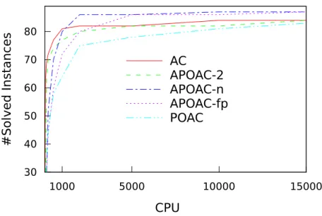
Table7and Figure5sum up the performance results obtained on all the in-stances with n-ary constraints. The binary classes are not included in the table and figure, because they have not been exhaustively tested. Figure5 gives the performance profile for each algorithm presented in Table 6: AC, APOAC-2, APOAC-n, APOAC-fp and POAC. Each point (t, i) on a curve indicates the number i of instances that an algorithm can solve in less than t seconds. The performance profile underlines that AC and APOAC are better than POAC: whatever the time given, they solve more instances than POAC. The compar-ison between AC and APOAC highlights two phases: A first phase (for easy instances), during which AC is better than APOAC, and a second phase, where APOAC becomes better than AC. Among the adaptive versions, APOAC-n is the variant with the shortest first phase (it adapts quite well to easy instances), and it remains the best even when time increases.
Finally, Table7compares the best APOAC version (APOAC-n) to AC and POAC on n-ary problems. The first row of the table gives the number of solved instances by each algorithm before the cuto↵. We observe that APOAC-n solves more instances than AC and POAC. The second row of the table gives the sum of CPU time required to solve all the instances. Again, when an instance cannot be solved before the cuto↵ of 15,000 seconds, we count 15,000 seconds for that instance. We observe that APOAC-n significantly outperforms both AC and POAC. The last two rows of the table give the gain of APOAC-n w.r.t. AC and w.r.t. POAC. We see that APOAC-n has a positive total gain greater than 51% compared to AC and greater than 76% compared to POAC.
7
Conclusion
We have proposed two approaches to adjust the level of consistency automat-ically during search. For the parameterized local consistency approach, we in-troduced the notion of stability of values for arc consistency, a notion based on the depth of their supports in their respective domain. This approach us allows us to define levels of local consistency of increasing strength between arc consistency and a given strong local consistency. We have introduced two techniques which allow us to make the parameter adaptable dynamically and
locally during search. As a second approach, we proposed POAC1, an algorithm that enforces partition-one-AC efficiently in practice. We have also proposed an adaptive version of POAC that monitors the number of variables on which to perform singleton tests. Our experiments show that in both approaches, adapt-ing the level of local consistency duradapt-ing search can outperform both MAC and maintaining a chosen local consistency stronger than AC.
Our approaches concentrate on adapting the level of consistency between the standard arc consistency and a chosen higher level. There are many constraints (especially global constraints) on which arc consistency is already a (too) high level of consistency and on which the standard consistency is bound consistency or some simple propagation rules. In these cases, an approach to that chosen in this paper could allow us to adapt automatically between arc consistency and the given lower level.
References
[BA01] H. Bennaceur and M.-S. A↵ane. Partition-k-AC: An Efficient Fil-tering Technique Combining Domain Partition and Arc Consistency. In Proceedings of the Seventh International Conference on Princi-ples and Practice of Constraint Programming (CP’01), LNCS 2239, Springer–Verlag, pages 560–564, Paphos, Cyprus, 2001.
[BBBT14] A. Balafrej, C. Bessiere, E.H. Bouyakhf, and G. Trombettoni. Adap-tive singleton-based consistencies. In Proceedings of the Twenty-Eighth AAAI Conference on Artificial Intelligence (AAAI’14), pages 2601–2607, Quebec City, Canada, 2014.
[BBCB13] A. Balafrej, C. Bessiere, R. Coletta, and E.H. Bouyakhf. Adaptive parameterized consistency. In Proceedings of the Eighteenth Inter-national Conference on Principles and Practice of Constraint Pro-gramming (CP’13), LNCS 8124, Springer–Verlag, pages 143–158, Uppsala, Sweden, 2013.
[BCDL11] C. Bessiere, S. Cardon, R. Debruyne, and C. Lecoutre. Efficient algorithms for singleton arc consistency. Constraints, 16(1):25–53, 2011.
[BD08] C. Bessiere and R. Debruyne. Theoretical analysis of singleton arc consistency and its extensions. Artif. Intell., 172(1):29–41, 2008. [Bes06] C. Bessiere. Constraint propagation. In F. Rossi, P. van Beek, and
T. Walsh, editors, Handbook of Constraint Programming, chapter 3. Elsevier, 2006.
[BHLS04] F. Boussemart, F. Hemery, C. Lecoutre, and L. Sais. Boosting systematic search by weighting constraints. In Proceedings of the Sixteenth European Conference on Artificial Intelligence (ECAI’04), pages 146–150, Valencia, Spain, 2004.
[BPSW11] T. Balafoutis, A. Paparrizou, K. Stergiou, and T. Walsh. New algo-rithms for max restricted path consistency. Constraints, 16(4):372– 406, 2011.
[BRYZ05] C. Bessiere, J. C. R´egin, R. H. C. Yap, and Y. Zhang. An Op-timal Coarse-grained Arc Consistency Algorithm. Artif. Intell., 165(2):165–185, 2005.
[BSW08] C. Bessiere, K. Stergiou, and T. Walsh. Domain filtering consis-tencies for non-binary constraints. Artif. Intell., 172(6-7):800–822, 2008.
[DB97] R. Debruyne and C. Bessiere. Some Practicable Filtering Techniques for the Constraint Satisfaction Problem. In Proceedings of the Fif-teenth International Joint Conference on Artificial Intelligence (IJ-CAI’97), pages 412–417, Nagoya, Japan, 1997.
[DB01] R. Debruyne and C. Bessiere. Domain filtering consistencies. Journal of Artificial Intelligence Research, 14:205–230, 2001.
[KVH06] I. Katriel and P. Van Hentenryck. Randomized filtering algorithms. Technical Report CS-06-09, Brown University, June 2006.
[NT13] B. Neveu and G. Trombettoni. Adaptive Constructive Interval Dis-junction. In Proceedings of the Twenty-Fifth IEEE International Conference on Tools for Artificial Intelligence (IEEE-ICTAI’13), pages 900–906, Washington D.C., USA, 2013.
[PS12] A. Paparrizou and K. Stergiou. Evaluating simple fully automated heuristics for adaptive constraint propagation. In Proceedings of the Twenty-Forth IEEE International Conference on Tools for Artifi-cial Intelligence (IEEE-ICTAI’12), pages 880–885, Athens, Greece, 2012.
[Sel03] M. Sellmann. Approximated consistency for knapsack constraints. In Proceedings of the Ninth International Conference on Princi-ples and Practice of Constraint Programming (CP’03), LNCS 2833, Springer–Verlag, pages 679–693, Kinsale, Ireland, 2003.
[SS09] E. Stamatatos and K. Stergiou. Learning how to propagate using random probing. In Proceedings of the Sixth International Confer-ence on Integration of AI and OR Techniques in Constraint Pro-gramming for Combinatorial Optimization Problems (CPAIOR’09), LNCS 5547, Springer, pages 263–278, Pittsburgh PA, 2009. [Ste08] K. Stergiou. Heuristics for dynamically adapting propagation. In
Proceedings of the Eighteenth European Conference on Artificial In-telligence (ECAI’08), pages 485–489, Patras, Greece, 2008.
[Ste09] K. Stergiou. Heuristics for dynamically adapting propagation in constraint satisfaction problems. AI Commun., 22:125–141, August 2009.
[TC07] G. Trombettoni and G. Chabert. Constructive Interval Disjunction. In Proceedings of the Thirteenth International Conference on Princi-ples and Practice of Constraint Programming (CP’07), LNCS 4741, Springer–Verlag, pages 635–650, Providence RI, 2007.
[VSD98] P. Van Hentenryck, V. A. Saraswat, and Y. Deville. Design, im-plementation, and evaluation of the constraint language cc(FD). J. Log. Program., 37(1-3):139–164, 1998.